Introduction to Algorithms. Second Edition. The MJT Press. Cambridge,
Massachusetts London, England. McGraw-Hill Book Company. Boston. Burr
Ridge, IL.
Thomas H. Cormen Charles E. Leiserson Ronald L. Rivest Clifford Stein
Introduction to Algorithms Second Edition
The MJT Press Cambridge, Massachusetts London, England McGraw-Hill Book Company Boston Burr Ridge, IL New York San Francisco
Dubuque, LA Madison, WI St. Louis Montdal Toronto
23
Minimum Spanning Trees
In the design of electronic circuitry, it is often necessary to make the pins of several components electrically equivalent by wiring them together. To interconnect a set of n pins, we can use an arrangement of n - 1 wires, each connecting two pins. Of all such arrangements, the one that uses the least amount of wire is usually the most desirable. We can model this wiring problem with a connected, undirected graph G = (V, E), where V is the set of pins, E is the set of possible interconnections between pairs of pins, and for each edge ( u , v) E E, we have a weight w(u, u ) specifying the cost (amount of wire needed) to connect u and u. We then wish to find an acyclic subset T 5 E that connects all of the vertices and whose total weight
is minimized. Since T is acyclic and connects all of the vertices, it must form a tree, which we call a spanning tree since it “spans” the graph G. We call the problem of determining the tree T the minimum-spanning-tree problem.’ Figure 23.1 shows an example of a connected graph and its minimum spanning tree. In this chapter, we shall examine two algorithms for solving the minimumspanning-tree problem: Kruskal’s algorithm and Prim’s algorithm. Each can easily be made to run in time O (E lg V) using ordinary binary heaps. By using Fibonacci heaps, Prim’s algorithm can be sped up to run in time O(E + V lg V), which is an improvement if IV I is much smaller than I E I. The two algorithms are greedy algorithms, as described in Chapter 16. At each step of an algorithm, one of several possible choices must be made. The greedy strategy advocates making the choice that is the best at the moment. Such a strategy is not generally guaranteed to find globally optimal solutions to problems. For The phrase “minimum spanning tree” is a shortened form of the phrase “minimum-weightspanning tree.” We are not, for example, minimizing the number of edges in T , since all spanning trees have exactly IV I - 1 edges by Theorem B.2.
562
Chapter 23 Minimum Spanning Trees
1
Figure 23.1 A minimum spanning tree for a connected graph. The weights on edges are shown, and the edges in a minimum spanning tree are shaded. The total weight of the tree shown is 37. This minimum spanning tree is not unique: removing the edge (b,c) and replacing it with the edge ( a , h ) yields another spanning tree with weight 37.
Cc
the minimum-spanning-tree problem, however, we can prove that certain greedy strategies do yield a spanning tree with minimum weight. Although the present chapter can be read independently of Chapter 16, the greedy methods presented here are a classic application of the theoretical notions introduced there. Section 23.1 introduces a “generic” minimum-spanning-tree algorithm that grows a spanning tree by adding one edge at a time. Section 23.2 gives two ways to implement the generic algorithm. The first algorithm, due to Kruskal, is similar to the connected-components algorithm from Section 21.1. The second, due to Prim, is similar to Dijkstra’s shortest-paths algorithm (Section 24.3).
23.1 Growing a minimum spanning tree Assume that we have a connected, undirected graph G = (V, E) with a weight function w : E + R,and we wish to find a minimum spanning tree for G. The two algorithms we consider in this chapter use a greedy approach to the problem, although they differ in how they apply this approach. This greedy strategy is captured by the following “generic” algorithm, which grows the minimum spanning tree one edge at a time. The algorithm manages a set of edges A, maintaining the following loop invariant: Prior to each iteration, A is a subset of some minimum spanning tree. At each step, we determine an edge (u, u ) that can be added to A without violating this invariant, in the sense that A U { (u, u ) ) is also a subset of a minimum spanning tree. We call such an edge a safe edge for A, since it can be safely added to A while maintaining the invariant.
23.1 Growing a minimum spanning tree
563
GENERIC-MST (G, W ) 1 A c 0 2 while A does not form a spanning tree do find an edge (u , u ) that is safe for A 3 4 A + A u {(u, u ) ) 5 return A We use the loop invariant as follows:
Initialization: After line 1, the set A trivially satisfies the loop invariant. Maintenance: The loop in lines 2-4 maintains the invariant by adding only safe edges. Termination: All edges added to A are in a minimum spanning tree, and so the set A is returned in line 5 must be a minimum spanning tree. The tricky part is, of course, finding a safe edge in line 3. One must exist, since when line 3 is executed, the invariant dictates that there is a spanning tree T such that A C T. Within the while loop body, A must be a proper subset of T, and therefore there must be an edge (u, u ) E T such that (u, u ) $ A and (u, u ) is safe for A. In the remainder of this section, we provide a rule (Theorem 23.1) for recognizing safe edges. The next section describes two algorithms that use this rule to find safe edges efficiently. We first need some definitions. A cut (S, V - S) of an undirected graph G = (V, E) is a partition of V. Figure 23.2 illustrates this notion. We say that an edge (u, v ) E E crosses the cut ( S , V - S) if one of its endpoints is in S and the other is in V - S. We say that a cut respects a set A of edges if no edge in A crosses the cut. An edge is a right edge crossing a cut if its weight is the minimum of any edge crossing the cut. Note that there can be more than one light edge crossing a cut in the case of ties. More generally, we say that an edge is a light edge satisfying a given property if its weight is the minimum of any edge satisfying the property. Our rule for recognizing safe edges is given by the following theorem. Theorem 23.1 Let G = (V, E) be a connected, undirected graph with a real-valued weight function w defined on E. Let A be a subset of E that is included in some minimum spanning tree for G, let (S, V - S) be any cut of G that respects A, and let (u, u ) be a light edge crossing (S, V - S). Then, edge (u, u ) is safe for A. Proof Let T be a minimum spanning tree that includes A, and assume that T does not contain the light edge (u, u), since if it does, we are done. We shall
‘“*I.
564
Chapter 23 Minimum Spanning Trees
-S
II I
* /I1I
Y in t
I1i
Figure 23.2 Two ways of viewing a cut (S, V - S)of the graph from Figure 23.1. (a) The vertices in the set S are shown in black, and those in V - S are shown in white. The edges crossing the cut are those connecting white vertices with black vertices. The edge ( d , c ) is the unique light edge crossing the cut. A subset A of the edges is shaded; note that the cut (S,V - S) respects A, since no edge of A crosses the cut. (b) The same graph with the vertices in the set S on the left and the vertices in the set V - S on the right. An edge crosses the cut if it C O M ~ C ~aSvertex on the left with a vertex on the right.
construct another minimum spanning tree TI that includes A U ((u, u ) } by using a cut-and-paste technique, thereby showing that (u, u ) is a safe edge for A. The edge (u, u ) forms a cycle with the edges on the path p fromu to u in T, as illustrated in Figure 23.3. Since u and u are on opposite sides of the cut (S, V - S), there is at least one edge in T on the path p that also crosses the cut. Let ( x , y) be any such edge. The edge ( x , y) is not in A, because the cut respects A. Since ( x , y) is on the unique path from u to u in T, removing ( x , y) breaks T into two components. Adding (u, u ) reconnects them to form a new spanning tree T’ = T - { ( x , Y ) } u {(u,4). We next show that TI is a minimum spanning tree. Since (u, u ) is a light edge crossing (S, V - S) and ( x , y) also crosses this cut, w(u, u ) 5 w ( x , y). Therefore,
w(T’) = w ( T ) - W ( X , y) h w(T).
+ ~ ( uU),
But T is a minimum spanning tree, so that w ( T ) 5 w(T’); thus, TI must be a minimum spanning tree also.
23.1 Growing a minimum spanning tree
565
A
‘\A /-
Figure 233 The proof of Theorem 23.1. The vertices in S are black, and the vertices in V - S are white. The edges in the minimum spanning tree T are shown, but the edges in the graph G are not. The edges in A are shaded, and (u, u ) is a light edge crossing the cut (S, V - S). The edge ( x , y ) is an edge on the unique path p from u to u in T. A minimum spanning tree TI that contains (u, u ) is formed by removing the edge (x, y) from T and adding the edge (u, u).
It remains to show that (u, v ) is actually a safe edge for A. We have A E T’, since A E T and ( x , y ) $ A; thus, A U ( ( u , v)} 5 TI. Consequently, since TI is a m minimum spanning tree, (u, v) is safe for A. Theorem 23.1 gives us a better understanding of the workings of the GENERIC-
MST algorithm on a connected graph G = (V, E). As the algorithm proceeds, the set A is always acyclic; otherwise, a minimum spanning tree including A would contain a cycle, which is a contradiction. At any point in the execution of the algorithm, the graph G A = (V, A ) is a forest, and each of the connected components of GA is a tree. (Some of the trees may contain just one vertex, as is the case, for example, when the algorithm begins: A is empty and the forest contains IVl trees, one for each vertex.) Moreover, any safe edge ( a , u) for A connects distinct components of G A ,since A U { ( u , v)) must be acyclic. The loop in lines 2 4 of GENERIC-MST is executed ( V (- 1 times as each of the IV I - 1 edges of a minimum spanning tree is successively determined. Initially, when A = 0, there are I V I trees in G A ,and each iteration reduces that number by 1. When the forest contains only a single tree,the algorithm terminates. The two algorithms in Section 23.2 use the following corollary to Theorem 23.1. Corollary 23.2 Let G = (V, E) be a connected, undirected graph with a real-valued weight function w defined on E. Let A be a subset of E that is included in some minimum spanning tree for G , and let C = (VC, Ec) be a connected component (tree) in
Chapter 23 Minimum Spanning Trees
566
the forest G A = (V, A). If (u, v ) is a light edge connecting C to some other component in GA, then ( u , v ) is safe for A.
Proof The cut (Vc, V - Vc) respects A, and (u, v ) is a light edge for this cut. Therefore, (u, v ) is safe for A. I
Exercises 23.1-1 Let ( u , v ) be a minimum-weight edge in a graph G. Show that (u, v ) belongs to some minimum spanning tree of G. 23.1-2 Professor Sabatier conjectures the following converse of Theorem 23.1. Let G = (V, E) be a connected, undirected graph with a real-valued weight function w defined on E. Let A be a subset of E that is included in some minimum spanning tree for G , let (S, V - S) be any cut of G that respects A, and let (u, v ) be a safe edge for A crossing (S, V - S). Then, (u, v ) is a light edge for the cut. Show that the professor's conjecture is incorrect by giving a counterexample. 23.1 -3 Show that if an edge (u, v ) is contained in some minimum spanning tree, then it is a light edge crossing some cut of the graph. 23.1-4 Give a simple example of a graph such that the set of edges { ( u , v ) : there exists a cut (S, V - S) such that (u, v ) is a light edge crossing (S, V - S)) does not form a minimum spanning tree. 23.1 -5 Let e be a maximum-weight edge on some cycle of G = (V, E). Prove that there is a minimum spanning tree of G' = ( V , E - {e})that is also a minimum spanning tree of G. That is, there is a minimum spanning tree of G that does not include e. 23.1 -6 Show that a graph has a unique minimum spanning tree if, for every cut of the graph, there is a unique light edge crossing the cut. Show that the converse is not true by giving a counterexample. 23.1 -7 Argue that if all edge weights of a graph are positive, then any subset of edges that connects all vertices and has minimum total weight must be a tree. Give an example
23.2 The algorithms of Kruskal and Prim
567
to show that the same conclusion does not follow if we allow some weights to be nonpositive.
23.1 -8 Let T be a minimum spanning tree of a graph G, and let L be the sorted list of the edge weights of T. Show that for any other minimum spanning tree T’ of G, the list L is also the sorted list of edge weights of TI. 23.1 -9 Let T be a minimum spanning tree of a graph G = (V, E), and let V’ be a subset of V. Let T’ be the subgraph of T induced by V’, and let G’be the subgraph of G induced by V’. Show that if T’ is connected, then T’ is a minimum spanning tree of GI. 23.1-10 Given a graph G and a minimum spanning tree T, suppose that we decrease the weight of one of the edges in T. Show that T is still a minimum spanning tree for G. More formally, let T be a minimum spanning tree for G with edge weights given by weight function w . Choose one edge ( x , y) E T and a positive number k, and define the weight function w‘ by
[ ~ ~i f ( u~,v)u ) #= ( x:, yy)) . ~ ~ - ~ if (u,
w’(u, v) =
(x,
,
Show that T is a minimum spanning tree for G with edge weights given by w’.
23.1-11 * Given a graph G and a minimum spanning tree T, suppose that we decrease the weight of one of the edges not in T. Give an algorithm for finding the minimum spanning tree in the modified graph.
23.2 The algorithms of Kruskal and Prim The two minimum-spanning-tree algorithms described in this section are elaborations of the generic algorithm. They each use a specific rule to determine a safe edge in line 3 of GENERIC-MST. In Kruskal’s algorithm, the set A is a forest. The safe edge added to A is always a least-weight edge in the graph that connects two distinct components. In Prim’s algorithm, the set A forms a single tree. The safe edge added to A is always a least-weight edge connecting the tree to a vertex not in the tree.
568
Chapter 23 Minimum Spanning Trees
Figure 23.4 The execution of Kruskal’s algorithm on the graph from Figure 23.1. Shaded edges belong to the forest A being grown. The edges are considered by the algorithm in sorted order by weight. An arrow points to the edge under consideration at each step of the algorithm. If the edge joins two distinct trees in the forest, it is added to the forest, thereby merging the two trees.
Kruskal’s algorithm Kruskal’s algorithm is based directly on the generic minimum-spanning-tree algorithm given in Section 23.1. It finds a safe edge to add to the growing forest by finding, of all the edges that connect any two trees in the forest, an edge (u, u ) of least weight. Let C1 and C2 denote the two trees that are connected by (u, u). Since ( u , v) must be a light edge connecting C1 to some other tree,Corollary 23.2
23.2 The algorithms of Kruskal and Prim
569 I
m
implies that ( u , v) is a safe edge for C1.Kruskal’s algorithm is a greedy algorithm, because at each step it adds to the forest an edge of least possible weight. Our implementation of Kruskal’s algorithm is like the algorithm to compute connected components from Section 21.1. It uses a disjoint-set data structure to maintain several disjoint sets of elements. Each set contains the vertices in a tree of the current forest. The operation FIND-SET(~) returns a representative element from the set that contains u. Thus, we can determine whether two vertices u and u belong to the same tree by testing whether FIND-SET(~) equals FIND-SET(U). The combining of trees is accomplished by the U NION procedure.
MST-KRUSKAL(G,W ) 1 A t 0 2 for each vertex v E V[G] 3 do MAKE-SET(V) 4 sort the edges of E into nondecreasing order by weight w 5 for each edge (u, v) E E, taken in nondecreasing order by weight 6 do if FIND-SET(U)# FIND-SET(U) 7 then A t A U {(u, v)} 8 UNION@,V ) 9 return A
t
i
Chapter 23 Minimum Spanning Trees
570
l
Kruskal’s algorithm works as shown in Figure 23.4. Lines 1-3 initialize the set A to the empty set and create IV I trees, one containing each vertex. The edges in E are sorted into nondecreasing order by weight in line 4. The for loop in lines 5-8 checks, for each edge (u, v ) , whether the endpoints u and v belong to the same tree. If they do, then the edge (u, v ) cannot be added to the forest without creating a cycle, and the edge is discarded. Otherwise, the two vertices belong to different trees. In this case, the edge ( u , v ) is added to A in line 7, and the vertices in the two trees are merged in line 8. The running time of Kruskal’s algorithm for a graph G = (V, E ) depends on the implementation of the disjoint-set data structure. We shall assume the disjoint-set-forest implementation of Section 21.3 with the union-by-rank and path-compression heuristics, since it is the asymptotically fastest implementation known. Initializing the set A in line 1 takes 0(1) time, and the time to sort the edges in line 4 is 0 ( E lg E ) . (We will account for the cost of the (V I MAKE-SET operations in the for loop of lines 2-3 in a moment.) The for loop of lines 5-8 performs 0( E ) FIND-SET and U NION operations on the disjoint-set forest. Along with the IV( M AKE-S ET operations, these take a total of O((V E ) a ( V ) )time, where a is the very slowly growing function defined in Section 21.4. Because G is assumed to be connected, we have IE I 2 IV I - 1, and so the disjoint-set operations take 0( E a ( V ) )time. Moreover, since a((V I) = 0(lg V) = 0 (Ig E ) , the total running time of Kruskal’s algorithm is O ( E 1gE). Observing that IEI < lV12, we have lg IEI = O(1g V), and so we can restate the running time of Kruskal’s algorithm as O ( E lg V).
+
Prim’s algorithm Like Kruskal’s algorithm, Prim’s algorithm is a special case of the generic minimum-spanning-tree algorithm from Section 23.1. Prim’s algorithm operates much like Dijkstra’s algorithm for finding shortest paths in a graph, which we shall see in Section 24.3. Prim’s algorithm has the property that the edges in the set A always form a single tree. As is illustrated in Figure 23.5, the tree starts from an arbitrary root vertex Y and grows until the tree spans all the vertices in V . At each step, a light edge is added to the tree A that connects A to an isolated vertex of G A = ( V , A). By Corollary 23.2, this rule adds only edges that are safe for A;
therefore, when the algorithm terminates, the edges in A form a minimum spanning tree. This strategy is greedy since the tree is augmented at each step with an edge that contributes the minimum amount possible to the tree’s weight. The key to implementing Prim’s algorithm efficiently is to make it easy to select a new edge to be added to the tree formed by the edges in A. In the pseudocode below, the connected graph G and the root r of the minimum spanning tree to be grown are inputs to the algorithm. During execution of the algorithm, all vertices
23.2 The algorithms of Kruskal and Prim
571
c
Figure 23.5 The execution of Prim’s algorithm on the graph from Figure 23.1. The root vertex is a. Shaded edges are in the tree being grown, and the vertices in the tree are shown in black. At each step of the algorithm, the vertices in the tree determine a cut of the graph, and a light edge crossing the cut is added to the tree. In the second step, for example, the algorithm has a choice of adding either edge (b, c) or edge ( a , h ) to the tree since both are light edges crossing the cut.
Chapter 23 Minimum Spanning Trees
572
that are not in the tree reside in a min-priority queue Q based on a key field. For each vertex u , key[v]is the minimum weight of any edge connecting u to a vertex in the tree; by convention, key[u] = 00 if there is no such edge. The field n[u]names the parent of u in the tree. During the algorithm, the set A from GENERIC-MST is kept implicitly as I
A = { ( v , ~ [ I I ] :) u E V - { r }- Q }
.
When the algorithm terminates, the min-priority queue Q is empty; the minimum spanning tree A for G is thus
A = { ( v , x [ v ] ): v E V - { r } } . MST-PRIM(G,W , t) 1 for each u E V [ G ] 2 do key[u] c 00 3 n [ u ]t NIL 4 key[r] c 0
5 Q+ W I 6 while Q # 0 7 do u c EXTRACT-MIN(Q) 8 for each u E Adj[u] 9 do if u E Q and w(u, v ) -= key[u] 10 then n[u] c u 11 keybl c W(U, v ) Prim’s algorithm works as shown in Figure 23.5. Lines 1-5 set the key of each vertex to 00 (except for the root r , whose key is set to 0 so that it will be the first vertex processed), set the parent of each vertex to NIL, and initialize the mhpriority queue Q to contain all the vertices. The algorithm maintains the following three-part loop invariant: Prior to each iteration of the while loop of lines 6-1 1, 1. A = { ( v , ~ [ v ]:)u E
V - {t}- Q}.
2. The vertices already placed into the minimum spanning tree are those in V - Q. 3. For all vertices u E Q , if n[u] # NIL, then k y [ u ] -= 00 and key[u] is the weight of a light edge ( u , n [ v ] )connecting u to some vertex already placed into the minimum spanning tree. Line 7 identifies a vertex u E Q incident on a light edge crossing the cut (V -Q,Q ) (with the exception of the first iteration, in which u = r due to line 4). Removing u
23.2 The algorithms of Kruskal and Prim
573
from the set Q adds it to the set V - Q of vertices in the tree, thus adding (u,n [ u ] ) to A. The for loop of lines 8-11 update the key and n fields of every vertex v adjacent to u but not in the tree. The updating maintains the third part of the loop invariant. The performance of Prim’s algorithm depends on how we implement the minpriority queue Q . If Q is implemented as a binary min-heap (see Chapter 6), we can use the B UILD -M IN -H EAP procedure to perform the initialization in lines 1-5 in O ( V ) time. The body of the while loop is executed IVl times, and since each EXTRACT-MIN operation takes O(1g V) time, the total time for all calls to EXTRACT-MIN is 0 (V lg V). The for loop in lines 8-1 1 is executed O(E)times altogether, since the sum of the lengths of all adjacency lists is 2 IEI. Within the for loop, the test for membership in Q in line 9 can be implemented in constant time by keeping a bit for each vertex that tells whether or not it is in Q,and updating the bit when the vertex is removed from Q. The assignment in line 11 involves an implicit D ECREASE-K EY operation on the min-heap, which can be implemented in a binary min-heap in O(1g V) time. Thus, the total time for Prim’s algorithm is O(V lg V E lg V) = 0 (E lg V), which is asymptotically the same as for our implementation of Kruskal’s algorithm. The asymptotic running time of Prim’s algorithm can be improved, however, by using Fibonacci heaps. Chapter 20 shows that if IV I elements are organized into a Fibonacci heap, we can perform an EXTRACT-MIN operation in O(1g V) amortized time and a D ECREASE-K EY operation (to implement line 11) in 0 (1) amortized time. Therefore, if we use a Fibonacci heap to implement the minpriority queue Q , the running time of Prim’s algorithm improves to 0 (E V lg V).
+
+
Exercises 23.2-1 Kruskal’s algorithm can return different spanning trees for the same input graph G, depending on how ties are broken when the edges are sorted into order. Show that for each minimum spanning tree T of G, there is a way to sort the edges of G in Kruskal’s algorithm so that the algorithm returns T. 23.2-2 Suppose that the graph G = (V, E) is represented as an adjacency matrix. Give a simple implementation of Prim’s algorithm for this case that runs in O ( V 2 )time. 23.2-3 Is the Fibonacci-heap implementation of Prim’s algorithm asymptotically faster than the binary-heap implementation for a sparse graph G = (V, E), where IEl = O(V)? What about for a dense graph, where {El = @(V*)?How must
( I
C
1
i