Introduction to Algorithms. 6.046J/18.401J. Prof. Charles E. Leiserson. LECTURE
14. Shortest Paths I. • Properties of shortest paths. • Dijkstra's algorithm.
Introduction to Algorithms 6.046J/18.401J
LECTURE 14 Shortest Paths I • Properties of shortest paths • Dijkstra’s algorithm • Correctness • Analysis • Breadth-first search Prof. Charles E. Leiserson
Paths in graphs Consider a digraph G = (V, E) with edge-weight function w : E → R. The weight of path p = v1 → v2 → L → vk is defined to be k −1
w( p ) = ∑ w(vi , vi +1 ) . i =1
© 2001–4 by Charles E. Leiserson
Introduction to Algorithms
November 1, 2004
L14.2
Paths in graphs Consider a digraph G = (V, E) with edge-weight function w : E → R. The weight of path p = v1 → v2 → L → vk is defined to be k −1
w( p ) = ∑ w(vi , vi +1 ) . i =1
Example:
vv11
4
vv22
–2
© 2001–4 by Charles E. Leiserson
vv33
–5
vv44
Introduction to Algorithms
1
vv55 w(p) = –2 November 1, 2004
L14.3
Shortest paths A shortest path from u to v is a path of minimum weight from u to v. The shortestpath weight from u to v is defined as δ(u, v) = min{w(p) : p is a path from u to v}. Note: δ(u, v) = ∞ if no path from u to v exists.
© 2001–4 by Charles E. Leiserson
Introduction to Algorithms
November 1, 2004
L14.4
Optimal substructure Theorem. A subpath of a shortest path is a shortest path.
© 2001–4 by Charles E. Leiserson
Introduction to Algorithms
November 1, 2004
L14.5
Optimal substructure Theorem. A subpath of a shortest path is a shortest path.
Proof. Cut and paste:
© 2001–4 by Charles E. Leiserson
Introduction to Algorithms
November 1, 2004
L14.6
Optimal substructure Theorem. A subpath of a shortest path is a shortest path.
Proof. Cut and paste:
© 2001–4 by Charles E. Leiserson
Introduction to Algorithms
November 1, 2004
L14.7
Triangle inequality Theorem. For all u, v, x ∈ V, we have δ(u, v) ≤ δ(u, x) + δ(x, v).
© 2001–4 by Charles E. Leiserson
Introduction to Algorithms
November 1, 2004
L14.8
Triangle inequality Theorem. For all u, v, x ∈ V, we have δ(u, v) ≤ δ(u, x) + δ(x, v).
Proof. δ(u, v)
uu δ(u, x)
vv δ(x, v)
xx © 2001–4 by Charles E. Leiserson
Introduction to Algorithms
November 1, 2004
L14.9
Well-definedness of shortest paths If a graph G contains a negative-weight cycle, then some shortest paths may not exist.
© 2001–4 by Charles E. Leiserson
Introduction to Algorithms
November 1, 2004
L14.10
Well-definedness of shortest paths If a graph G contains a negative-weight cycle, then some shortest paths may not exist. Example:
… d[u] + w(u, v) then d[v] ← d[u] + w(u, v)
© 2001–4 by Charles E. Leiserson
Introduction to Algorithms
November 1, 2004
L14.14
Dijkstra’s algorithm d[s] ← 0 for each v ∈ V – {s} do d[v] ← ∞ S←∅ Q←V ⊳ Q is a priority queue maintaining V – S while Q ≠ ∅ do u ← EXTRACT-MIN(Q) S ← S ∪ {u} for each v ∈ Adj[u] relaxation do if d[v] > d[u] + w(u, v) then d[v] ← d[u] + w(u, v) step
Implicit DECREASE-KEY © 2001–4 by Charles E. Leiserson
Introduction to Algorithms
November 1, 2004
L14.15
Example of Dijkstra’s algorithm Graph with nonnegative edge weights:
10
AA
1 4 3
© 2001–4 by Charles E. Leiserson
BB
Introduction to Algorithms
CC
2 8
2
D D 7 9
EE
November 1, 2004
L14.16
Example of Dijkstra’s algorithm ∞ BB
Initialize: 10
0 AA Q: A B C D E 0
∞
∞
∞
1 4 3
∞
CC ∞
2 8
2
∞ D D 7 9
EE ∞
S: {} © 2001–4 by Charles E. Leiserson
Introduction to Algorithms
November 1, 2004
L14.17
Example of Dijkstra’s algorithm “A” ← EXTRACT-MIN(Q): 10
0 AA Q: A B C D E 0
∞
∞
∞
∞ BB
1 4 3
∞
CC ∞
2 8
2
∞ D D 7 9
EE ∞
S: { A } © 2001–4 by Charles E. Leiserson
Introduction to Algorithms
November 1, 2004
L14.18
Example of Dijkstra’s algorithm Relax all edges leaving A: 10
0 AA Q: A B C D E 0
∞ 10
∞ 3
∞ ∞
10 BB
1 4 3
∞ ∞
CC 3
2 8
2
∞ D D 7 9
EE ∞
S: { A } © 2001–4 by Charles E. Leiserson
Introduction to Algorithms
November 1, 2004
L14.19
Example of Dijkstra’s algorithm “C” ← EXTRACT-MIN(Q): 10
0 AA Q: A B C D E 0
∞ 10
∞ 3
∞ ∞
10 BB
2 8
1 4 3
∞ ∞
CC 3
2
∞ D D 7 9
EE ∞
S: { A, C } © 2001–4 by Charles E. Leiserson
Introduction to Algorithms
November 1, 2004
L14.20
Example of Dijkstra’s algorithm Relax all edges leaving C: 10
0 AA Q: A B C D E 0
∞ 10 7
∞ 3
© 2001–4 by Charles E. Leiserson
∞ ∞ 11
∞ ∞ 5
7 BB
2 8
1 4 3
CC 3
2
11 D D 7 9
EE 5
S: { A, C }
Introduction to Algorithms
November 1, 2004
L14.21
Example of Dijkstra’s algorithm “E” ← EXTRACT-MIN(Q): 10
0 AA Q: A B C D E 0
∞ 10 7
∞ 3
© 2001–4 by Charles E. Leiserson
∞ ∞ 11
∞ ∞ 5
7 BB
1 4 3
CC 3
2 8
2
11 D D 7 9
EE 5
S: { A, C, E }
Introduction to Algorithms
November 1, 2004
L14.22
Example of Dijkstra’s algorithm Relax all edges leaving E: 10
0 AA Q: A B C D E 0
∞ 10 7 7
∞ 3
© 2001–4 by Charles E. Leiserson
∞ ∞ 11 11
∞ ∞ 5
7 BB
1 4 3
CC 3
2 8
2
11 D D 7 9
EE 5
S: { A, C, E }
Introduction to Algorithms
November 1, 2004
L14.23
Example of Dijkstra’s algorithm “B” ← EXTRACT-MIN(Q): 10
0 AA Q: A B C D E 0
∞ 10 7 7
∞ 3
© 2001–4 by Charles E. Leiserson
∞ ∞ 11 11
∞ ∞ 5
7 BB
1 4 3
CC 3
2 8
11 D D 7 9
2
EE 5
S: { A, C, E, B }
Introduction to Algorithms
November 1, 2004
L14.24
Example of Dijkstra’s algorithm Relax all edges leaving B: 10
0 AA Q: A B C D E 0
∞ 10 7 7
∞ 3
© 2001–4 by Charles E. Leiserson
∞ ∞ 11 11 9
∞ ∞ 5
7 BB
1 4 3
CC 3
9 D D
2 8
7 9
2
EE 5
S: { A, C, E, B }
Introduction to Algorithms
November 1, 2004
L14.25
Example of Dijkstra’s algorithm “D” ← EXTRACT-MIN(Q): 10
0 AA Q: A B C D E 0
∞ 10 7 7
∞ 3
© 2001–4 by Charles E. Leiserson
∞ ∞ 11 11 9
∞ ∞ 5
7 BB
1 4 3
CC 3
2 8
2
9 D D 7 9
EE 5
S: { A, C, E, B, D }
Introduction to Algorithms
November 1, 2004
L14.26
Correctness — Part I Lemma. Initializing d[s] ← 0 and d[v] ← ∞ for all v ∈ V – {s} establishes d[v] ≥ δ(s, v) for all v ∈ V, and this invariant is maintained over any sequence of relaxation steps.
© 2001–4 by Charles E. Leiserson
Introduction to Algorithms
November 1, 2004
L14.27
Correctness — Part I Lemma. Initializing d[s] ← 0 and d[v] ← ∞ for all v ∈ V – {s} establishes d[v] ≥ δ(s, v) for all v ∈ V, and this invariant is maintained over any sequence of relaxation steps. Proof. Suppose not. Let v be the first vertex for which d[v] < δ(s, v), and let u be the vertex that caused d[v] to change: d[v] = d[u] + w(u, v). Then, d[v] < δ(s, v) supposition ≤ δ(s, u) + δ(u, v) triangle inequality ≤ δ(s,u) + w(u, v) sh. path ≤ specific path ≤ d[u] + w(u, v) v is first violation Contradiction. © 2001–4 by Charles E. Leiserson
Introduction to Algorithms
November 1, 2004
L14.28
Correctness — Part II Lemma. Let u be v’s predecessor on a shortest path from s to v. Then, if d[u] = δ(s, u) and edge (u, v) is relaxed, we have d[v] = δ(s, v) after the relaxation.
© 2001–4 by Charles E. Leiserson
Introduction to Algorithms
November 1, 2004
L14.29
Correctness — Part II Lemma. Let u be v’s predecessor on a shortest path from s to v. Then, if d[u] = δ(s, u) and edge (u, v) is relaxed, we have d[v] = δ(s, v) after the relaxation. Proof. Observe that δ(s, v) = δ(s, u) + w(u, v). Suppose that d[v] > δ(s, v) before the relaxation. (Otherwise, we’re done.) Then, the test d[v] > d[u] + w(u, v) succeeds, because d[v] > δ(s, v) = δ(s, u) + w(u, v) = d[u] + w(u, v), and the algorithm sets d[v] = d[u] + w(u, v) = δ(s, v). © 2001–4 by Charles E. Leiserson
Introduction to Algorithms
November 1, 2004
L14.30
Correctness — Part III Theorem. Dijkstra’s algorithm terminates with d[v] = δ(s, v) for all v ∈ V.
© 2001–4 by Charles E. Leiserson
Introduction to Algorithms
November 1, 2004
L14.31
Correctness — Part III Theorem. Dijkstra’s algorithm terminates with d[v] = δ(s, v) for all v ∈ V. Proof. It suffices to show that d[v] = δ(s, v) for every v ∈ V when v is added to S. Suppose u is the first vertex added to S for which d[u] > δ(s, u). Let y be the first vertex in V – S along a shortest path from s to u, and let x be its predecessor:
uu S, just before adding u. © 2001–4 by Charles E. Leiserson
ss Introduction to Algorithms
xx
yy November 1, 2004
L14.32
Correctness — Part III (continued) S ss
uu xx
yy
Since u is the first vertex violating the claimed invariant, we have d[x] = δ(s, x). When x was added to S, the edge (x, y) was relaxed, which implies that d[y] = δ(s, y) ≤ δ(s, u) < d[u]. But, d[u] ≤ d[y] by our choice of u. Contradiction. © 2001–4 by Charles E. Leiserson
Introduction to Algorithms
November 1, 2004
L14.33
Analysis of Dijkstra while Q ≠ ∅ do u ← EXTRACT-MIN(Q) S ← S ∪ {u} for each v ∈ Adj[u] do if d[v] > d[u] + w(u, v) then d[v] ← d[u] + w(u, v)
© 2001–4 by Charles E. Leiserson
Introduction to Algorithms
November 1, 2004
L14.34
Analysis of Dijkstra |V | times
while Q ≠ ∅ do u ← EXTRACT-MIN(Q) S ← S ∪ {u} for each v ∈ Adj[u] do if d[v] > d[u] + w(u, v) then d[v] ← d[u] + w(u, v)
© 2001–4 by Charles E. Leiserson
Introduction to Algorithms
November 1, 2004
L14.35
Analysis of Dijkstra |V | times
while Q ≠ ∅ do u ← EXTRACT-MIN(Q) S ← S ∪ {u} for each v ∈ Adj[u] degree(u) do if d[v] > d[u] + w(u, v) times then d[v] ← d[u] + w(u, v)
© 2001–4 by Charles E. Leiserson
Introduction to Algorithms
November 1, 2004
L14.36
Analysis of Dijkstra |V | times
while Q ≠ ∅ do u ← EXTRACT-MIN(Q) S ← S ∪ {u} for each v ∈ Adj[u] degree(u) do if d[v] > d[u] + w(u, v) times then d[v] ← d[u] + w(u, v)
Handshaking Lemma ⇒ Θ(E) implicit DECREASE-KEY’s.
© 2001–4 by Charles E. Leiserson
Introduction to Algorithms
November 1, 2004
L14.37
Analysis of Dijkstra |V | times
while Q ≠ ∅ do u ← EXTRACT-MIN(Q) S ← S ∪ {u} for each v ∈ Adj[u] degree(u) do if d[v] > d[u] + w(u, v) times then d[v] ← d[u] + w(u, v)
Handshaking Lemma ⇒ Θ(E) implicit DECREASE-KEY’s.
Time = Θ(V·TEXTRACT-MIN + E·TDECREASE-KEY) Note: Same formula as in the analysis of Prim’s minimum spanning tree algorithm. © 2001–4 by Charles E. Leiserson
Introduction to Algorithms
November 1, 2004
L14.38
Analysis of Dijkstra (continued) Time = Θ(V)·TEXTRACT-MIN + Θ(E)·TDECREASE-KEY Q
TEXTRACT-MIN TDECREASE-KEY
© 2001–4 by Charles E. Leiserson
Introduction to Algorithms
Total
November 1, 2004
L14.39
Analysis of Dijkstra (continued) Time = Θ(V)·TEXTRACT-MIN + Θ(E)·TDECREASE-KEY Q array
TEXTRACT-MIN TDECREASE-KEY O(V)
© 2001–4 by Charles E. Leiserson
O(1)
Introduction to Algorithms
Total O(V2)
November 1, 2004
L14.40
Analysis of Dijkstra (continued) Time = Θ(V)·TEXTRACT-MIN + Θ(E)·TDECREASE-KEY Q
TEXTRACT-MIN TDECREASE-KEY
Total
array
O(V)
O(1)
O(V2)
binary heap
O(lg V)
O(lg V)
O(E lg V)
© 2001–4 by Charles E. Leiserson
Introduction to Algorithms
November 1, 2004
L14.41
Analysis of Dijkstra (continued) Time = Θ(V)·TEXTRACT-MIN + Θ(E)·TDECREASE-KEY Q
TEXTRACT-MIN TDECREASE-KEY
Total
array
O(V)
O(1)
O(V2)
binary heap
O(lg V)
O(lg V)
O(E lg V)
Fibonacci O(lg V) heap amortized © 2001–4 by Charles E. Leiserson
O(1) O(E + V lg V) amortized worst case
Introduction to Algorithms
November 1, 2004
L14.42
Unweighted graphs Suppose that w(u, v) = 1 for all (u, v) ∈ E. Can Dijkstra’s algorithm be improved?
© 2001–4 by Charles E. Leiserson
Introduction to Algorithms
November 1, 2004
L14.43
Unweighted graphs Suppose that w(u, v) = 1 for all (u, v) ∈ E. Can Dijkstra’s algorithm be improved? • Use a simple FIFO queue instead of a priority queue.
© 2001–4 by Charles E. Leiserson
Introduction to Algorithms
November 1, 2004
L14.44
Unweighted graphs Suppose that w(u, v) = 1 for all (u, v) ∈ E. Can Dijkstra’s algorithm be improved? • Use a simple FIFO queue instead of a priority queue. Breadth-first search while Q ≠ ∅ do u ← DEQUEUE(Q) for each v ∈ Adj[u] do if d[v] = ∞ then d[v] ← d[u] + 1 ENQUEUE(Q, v)
© 2001–4 by Charles E. Leiserson
Introduction to Algorithms
November 1, 2004
L14.45
Unweighted graphs Suppose that w(u, v) = 1 for all (u, v) ∈ E. Can Dijkstra’s algorithm be improved? • Use a simple FIFO queue instead of a priority queue. Breadth-first search while Q ≠ ∅ do u ← DEQUEUE(Q) for each v ∈ Adj[u] do if d[v] = ∞ then d[v] ← d[u] + 1 ENQUEUE(Q, v)
Analysis: Time = O(V + E). © 2001–4 by Charles E. Leiserson
Introduction to Algorithms
November 1, 2004
L14.46
Example of breadth-first search aa
ff
hh
dd bb
gg ee
ii
cc Q: © 2001–4 by Charles E. Leiserson
Introduction to Algorithms
November 1, 2004
L14.47
Example of breadth-first search 0
aa
ff
hh
dd bb
gg ee
ii
cc 0
Q: a © 2001–4 by Charles E. Leiserson
Introduction to Algorithms
November 1, 2004
L14.48
Example of breadth-first search 0
aa
1
ff
hh
dd 1
bb
gg ee
ii
cc 1 1
Q: a b d © 2001–4 by Charles E. Leiserson
Introduction to Algorithms
November 1, 2004
L14.49
Example of breadth-first search 0
aa
1
ff
hh
dd 1
bb
gg ee
2
cc
ii
2 1 2 2
Q: a b d c e © 2001–4 by Charles E. Leiserson
Introduction to Algorithms
November 1, 2004
L14.50
Example of breadth-first search 0
aa
ff
1
hh
dd 1
bb
gg ee
2
cc
ii
2 2 2
Q: a b d c e © 2001–4 by Charles E. Leiserson
Introduction to Algorithms
November 1, 2004
L14.51
Example of breadth-first search 0
aa
ff
1
hh
dd 1
bb
gg ee
2
cc
ii
2 2
Q: a b d c e © 2001–4 by Charles E. Leiserson
Introduction to Algorithms
November 1, 2004
L14.52
Example of breadth-first search 0
aa
dd 1
2
bb cc
ff
1 3
hh
gg
ee
ii
2
3 3 3
Q: a b d c e g i © 2001–4 by Charles E. Leiserson
Introduction to Algorithms
November 1, 2004
L14.53
Example of breadth-first search 4 0
aa
dd 1
2
bb cc
ff
1 3
hh
gg
ee
ii
2
3 3 4
Q: a b d c e g i f © 2001–4 by Charles E. Leiserson
Introduction to Algorithms
November 1, 2004
L14.54
Example of breadth-first search 0
aa
1
dd 1
2
bb cc
3
4
4
ff
hh
gg
ee
ii
2
3 4 4
Q: a b d c e g i f h © 2001–4 by Charles E. Leiserson
Introduction to Algorithms
November 1, 2004
L14.55
Example of breadth-first search 0
aa
1
dd 1
2
bb cc
3
4
4
ff
hh
gg
ee
ii
2
3 4
Q: a b d c e g i f h © 2001–4 by Charles E. Leiserson
Introduction to Algorithms
November 1, 2004
L14.56
Example of breadth-first search 0
aa
1
dd 1
2
bb cc
3
4
4
ff
hh
gg
ee
ii
2
3
Q: a b d c e g i f h © 2001–4 by Charles E. Leiserson
Introduction to Algorithms
November 1, 2004
L14.57
Example of breadth-first search 0
aa
1
dd 1
2
bb cc
3
4
4
ff
hh
gg
ee
ii
2
3
Q: a b d c e g i f h © 2001–4 by Charles E. Leiserson
Introduction to Algorithms
November 1, 2004
L14.58
Correctness of BFS while Q ≠ ∅ do u ← DEQUEUE(Q) for each v ∈ Adj[u] do if d[v] = ∞ then d[v] ← d[u] + 1 ENQUEUE(Q, v)
Key idea: The FIFO Q in breadth-first search mimics the priority queue Q in Dijkstra. • Invariant: v comes after u in Q implies that d[v] = d[u] or d[v] = d[u] + 1. © 2001–4 by Charles E. Leiserson
Introduction to Algorithms
November 1, 2004
L14.59