Introduction to General and Generalized Linear Models - DTU

Introduction to General and Generalized Linear Models General Linear Models - part I

Henrik Madsen Poul Thyregod Informatics and Mathematical Modelling Technical University of Denmark DK-2800 Kgs. Lyngby

October 2010

Henrik MadsenPoul Thyregod (IMM-DTU)

Chapman & Hall

October 2010

1 / 37

Today The general linear model - intro The multivariate normal distribution Deviance Likelihood, score function and information matrix The general linear model - definition Estimation Fitted values Residuals Partitioning of variation Likelihood ratio tests The coefficient of determination

Henrik MadsenPoul Thyregod (IMM-DTU)

Chapman & Hall

October 2010

2 / 37

The general linear model - intro

The general linear model - intro

We will use the term classical GLM for the General linear model to distinguish it from GLM which is used for the Generalized linear model. The classical GLM leads to a unique way of describing the variations of experiments with a continuous variable. The classical GLM’s include Regression analysis Analysis of variance - ANOVA Analysis of covariance - ANCOVA

The residuals are assumed to follow a multivariate normal distribution in the classical GLM.

Henrik MadsenPoul Thyregod (IMM-DTU)

Chapman & Hall

October 2010

3 / 37

The general linear model - intro

The general linear model - intro

Classical GLM’s are naturally studied in the framework of the multivariate normal distribution. We will consider the set of n observations as a sample from a n-dimensional normal distribution. Under the normal distribution model, maximum-likelihood estimation of mean value parameters may be interpreted geometrically as projection on an appropriate subspace. The likelihood-ratio test statistics for model reduction may be expressed in terms of norms of these projections.

Henrik MadsenPoul Thyregod (IMM-DTU)

Chapman & Hall

October 2010

4 / 37

The multivariate normal distribution

The multivariate normal distribution Let Y = (Y1 , Y2 , . . . , Yn )T be a random vector with Y1 , Y2 , . . . , Yn independent identically distributed (iid) N(0, 1) random variables. Note that E[Y ] = 0 and the variance-covariance matrix Var[Y ] = I. Definition (Multivariate normal distribution) Z has an k-dimensional multivariate normal distribution if Z has the same distribution as AY + b for some n, some k × n matrix A, and some k vector b. We indicate the multivariate normal distribution by writing Z ∼ N(b, AAT ). Since A and b are fixed, we have E[Z] = b and Var[Z] = AAT .

Henrik MadsenPoul Thyregod (IMM-DTU)

Chapman & Hall

October 2010

5 / 37

The multivariate normal distribution

The multivariate normal distribution

Let us assume that the variance-covariance matrix is known apart from a constant factor, σ 2 , i.e. Var[Z] = σ 2 Σ. The density for the k-dimensional random vector Z with mean µ and covariance σ 2 Σ is:   1 1 T −1 √ fZ (z) = exp − 2 (z − µ) Σ (z − µ) 2σ (2π)k/2 σ k det Σ where Σ is seen to be (a) symmetric and (b) positive semi-definite. We write Z ∼ Nk (µ, σ 2 Σ).

Henrik MadsenPoul Thyregod (IMM-DTU)

Chapman & Hall

October 2010

6 / 37

The multivariate normal distribution

The normal density as a statistical model

Consider now the n observations Y = (Y1 , Y2 , . . . , Yn )T , and assume that a statistical model is Y ∼ Nn (µ, σ 2 Σ) for y ∈ Rn The variance-covariance matrix for the observations is called the dispersion matrix, denoted D[Y ], i.e. the dispersion matrix for Y is D[Y ] = σ 2 Σ

Henrik MadsenPoul Thyregod (IMM-DTU)

Chapman & Hall

October 2010

7 / 37

Inner product and norm

Inner product and norm

Definition (Inner product and norm) The bilinear form δΣ (y1 , y2 ) = y1T Σ−1 y2 defines an inner product in Rn . Corresponding to this inner product we can define orthogonality, which is obtained when the inner product is zero. A norm is defined by ||y||Σ =

Henrik MadsenPoul Thyregod (IMM-DTU)

p δΣ (y, y).

Chapman & Hall

October 2010

8 / 37

Deviance

Deviance for normal distributed variables

Definition (Deviance for normal distributed variables) Let us introduce the notation D(y; µ) = δΣ (y − µ, y − µ) = (y − µ)T Σ−1 (y − µ) to denote the quadratic norm of the vector (y − µ) corresponding to the inner product defined by Σ−1 . For a normal distribution with Σ = I, the deviance is just the Residual Sum of Squares (RSS).

Henrik MadsenPoul Thyregod (IMM-DTU)

Chapman & Hall

October 2010

9 / 37

Deviance

Deviance for normal distributed variables

Using this notation the normal density is expressed as a density defined on any finite dimensional vector space equipped with the inner product, δΣ :   1 1 2 p f (y; µ, σ ) = √ exp − 2 D(y; µ) . 2σ ( 2π)n σ n det(Σ)

Henrik MadsenPoul Thyregod (IMM-DTU)

Chapman & Hall

October 2010

10 / 37

Likelihood, score function and information matrix

The likelihood and log-likelihood function

The likelihood function is:

  1 1 p exp − 2 D(y; µ) L(µ, σ ; y) = √ 2σ ( 2π)n σ n det(Σ) 2

The log-likelihood function is (apart from an additive constant): 1 (y − µ)T Σ−1 (y − µ) 2σ 2 1 = −(n/2) log(σ 2 ) − 2 D(y; µ). 2σ

`µ,σ2 (µ, σ 2 ; y) = −(n/2) log(σ 2 ) −

Henrik MadsenPoul Thyregod (IMM-DTU)

Chapman & Hall

October 2010

11 / 37

Likelihood, score function and information matrix

The score function, observed - and expected information for µ The score function wrt. µ is  ∂ 1  1 `µ,σ2 (µ, σ 2 ; y) = 2 Σ−1 y − Σ−1 µ = 2 Σ−1 (y − µ) ∂µ σ σ The observed information (wrt. µ) is j(µ; y) =

1 −1 Σ . σ2

It is seen that the observed information does not depend on the observations y. Hence the expected information is i(µ) =

Henrik MadsenPoul Thyregod (IMM-DTU)

1 −1 Σ . σ2

Chapman & Hall

October 2010

12 / 37

The general linear model

The general linear model

In the case of a normal density the observation Yi is most often written as Yi = µi + i which for all n observations (Y1 , Y2 , . . . , Yn ) can be written on the matrix form Y =µ+ where Y ∼ Nn (µ, σ 2 Σ) for y ∈ Rn

Henrik MadsenPoul Thyregod (IMM-DTU)

Chapman & Hall

October 2010

13 / 37

The general linear model

General Linear Models In the linear model it is assumed that µ belongs to a linear (or affine) subspace Ω0 of Rn . The full model is a model with Ωf ull = Rn and hence each b = y. observation fits the model perfectly, i.e. µ The most restricted model is the null model with Ωnull = R. It only describes the variations of the observations by a common mean value for all observations. In practice, one often starts with formulating a rather comprehensive model with Ω = Rk , where k < n. We will call such a model a sufficient model.

Henrik MadsenPoul Thyregod (IMM-DTU)

Chapman & Hall

October 2010

14 / 37

The general linear model

The General Linear Model Definition (The general linear model) Assume that Y1 , Y2 , . . . , Yn is normally distributed as described before. A general linear model for Y1 , Y2 , . . . , Yn is a model where an affine hypothesis is formulated for µ. The hypothesis is of the form H0 : µ − µ 0 ∈ Ω 0 , where Ω0 is a linear subspace of Rn of dimension k, and where µ0 denotes a vector of known offset values. Definition (Dimension of general linear model) The dimension of the subspace Ω0 for the linear model is the dimension of the model.

Henrik MadsenPoul Thyregod (IMM-DTU)

Chapman & Hall

October 2010

15 / 37

The general linear model

The design matrix Definition (Design matrix for classical GLM) Assume that the linear subspace Ω0 = span{x1 , . . . , xk }, i.e. the subspace is spanned by k vectors (k < n). Consider a general linear model where the hypothesis can be written as H0 : µ − µ0 = Xβ with β ∈ Rk , where X has full rank. The n × k matrix X of known deterministic coefficients is called the design matrix. The ith row of the design matrix is given by the model vector    xTi =  

xi1 xi2 .. .

T    , 

xik for the ith observation. Henrik MadsenPoul Thyregod (IMM-DTU)

Chapman & Hall

October 2010

16 / 37

Estimation

Estimation of mean value parameters Under the hypothesis H0 : µ ∈ Ω 0 , the maximum likelihood estimate for the set µ is found as the orthogonal projection (with respect to δΣ ), p0 (y) of y onto the linear subspace Ω0 . Theorem (ML estimates of mean value parameters) For hypothesis of the form H0 : µ(β) = Xβ the maximum likelihood estimated for β is found as a solution to the normal equation b X T Σ−1 y = X T Σ−1 X β. If X has full rank, the solution is uniquely given by βb = (X T Σ−1 X)−1 X T Σ−1 y Henrik MadsenPoul Thyregod (IMM-DTU)

Chapman & Hall

October 2010

17 / 37

Estimation

Properties of the ML estimator

Theorem (Properties of the ML estimator) For the ML estimator we have βb ∼ Nk (β, σ 2 (X T Σ−1 X)−1 ) Unknown Σ Notice that it has been assumed that Σ is known. If Σ is unknown, one possibility is to use the relaxation algorithm described in Madsen (2008) a . a

Madsen, H. (2008) Time Series Analysis. Chapman, Hall

Henrik MadsenPoul Thyregod (IMM-DTU)

Chapman & Hall

October 2010

18 / 37

Fitted values

Fitted values

Fitted – or predicted – values b = X βb is found as the projection of y (denoted p0 (y)) The fitted values µ on to the subspace Ω0 spanned by X, and βb denotes the local coordinates for the projection. Definition (Projection matrix) A matrix H is a projection matrix if and only if (a) H T = H and (b) H 2 = H, i.e. the matrix is idempotent.

Henrik MadsenPoul Thyregod (IMM-DTU)

Chapman & Hall

October 2010

19 / 37

Fitted values

The hat matrix The matrix H = X[X T Σ−1 X]−1 X T Σ−1 is a projection matrix. b since The projection matrix provides the predicted values µ, b = p0 (y) = X βb = Hy µ It follows that the predicted values are normally distributed with b = σ 2 X[X T Σ−1 X]−1 X T = σ 2 HΣ D[Xβ] The matrix H is often termed the hat matrix since it transforms the observations y to their predicted values symbolized by a ”hat” on the µ’s. Henrik MadsenPoul Thyregod (IMM-DTU)

Chapman & Hall

October 2010

20 / 37

Residuals

Residuals The observed residuals are r = y − X βb = (I − H)y Orthogonality The maximum likelihood estimate for β is found as the value of β which minimizes the distance ||y − Xβ||. The normal equations show that b =0 X T Σ−1 (y − X β) i.e. the residuals are orthogonal (with respect to Σ−1 ) to the subspace Ω0 . The residuals are thus orthogonal to the fitted – or predicted – values. Henrik MadsenPoul Thyregod (IMM-DTU)

Chapman & Hall

October 2010

21 / 37

Residuals

Residuals 3.5 Likelihood ratio tests

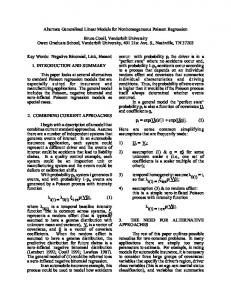
45 y

kyk

Ω0 0

kp0 (y)k

ky − po (y)k

p0 (y) = X βb

b and the vector X β. b Figure 3.1: Orthogonality between the residual (y − X β)

b and the vector X β. b Figure: Orthogonality between the residual (y − X β)

Henrik MadsenPoul Thyregod (IMM-DTU)

Chapman & Hall

October 2010

22 / 37

Residuals

Residuals

The residuals r = (I − H)Y are normally distributed with D[r] = σ 2 (I − H) The individual residuals do not have the same variance. The residuals are thus belonging to a subspace of dimension n − k, which is orthogonal to Ω0 . It may be shown that the distribution of the residuals r is b independent of the fitted values X β.

Henrik MadsenPoul Thyregod (IMM-DTU)

Chapman & Hall

October 2010

23 / 37

Residuals

Cochran’s theorem Theorem (Cochran’s theorem) Suppose that Y ∼ Nn (0, In ) (i.e. standard multivariate Gaussian random variable) Y T Y = Y T H1 Y + Y T H2 Y + · · · + Y T Hk Y where Hi is a symmetric n × n matrix with rank ni , i = 1, 2, . . . , k. Then any one of the following conditions implies the other two: Pk i The ranks of the Hi adds to n, i.e. i=1 ni = n ii Each quadratic form Y T Hi Y ∼ χ2ni (thus the Hi are positive semidefinite) iii All the quadratic forms Y T Hi Y are independent (necessary and sufficient condition). Henrik MadsenPoul Thyregod (IMM-DTU)

Chapman & Hall

October 2010

24 / 37

Partitioning of variation

Partitioning of variation

Partitioning of the variation b + D(X β; b Xβ) D(y; Xβ) = D(y; X β) b T Σ−1 (y − X β) b = (y − X β) + (βb − β)T X T Σ−1 X(βb − β) b T Σ−1 (y − X β) b ≥ (y − X β)

Henrik MadsenPoul Thyregod (IMM-DTU)

Chapman & Hall

October 2010

25 / 37

Partitioning of variation

Partitioning of variation χ2 -distribution of individual contributions Under H0 it follows from the normal distribution of Y that D(y; Xβ) = (y − Xβ)T Σ−1 (y − Xβ) ∼ σ 2 χ2n Furthermore, it follows from the normal distribution of r and of βb that b = (y − X β) b T Σ−1 (y − X β) b ∼ σ 2 χ2 D(y; X β) n−k T T −1 2 2 b b b D(X β; Xβ) = (β − β) X Σ X(β − β) ∼ σ χ k

b and moreover, the independence of r and X βb implies that D(y; X β) b Xβ) are independent. D(X β; Thus, the σ 2 χ2n -distribution on the left side is partitioned into two independent χ2 distributed variables with n − k and k degrees of freedom, respectively. Henrik MadsenPoul Thyregod (IMM-DTU)

Chapman & Hall

October 2010

26 / 37

Estimation of the residual variance σ 2

Estimation of the residual variance σ 2

Theorem (Estimation of the variance) Under the hypothesis H0 : µ(β) = Xβ the maximum marginal likelihood estimator for the variance σ 2 is σ b2 =

b b T Σ−1 (y − X β) b D(y; X β) (y − X β) = n−k n−k

Under the hypothesis, σ b2 ∼ σ 2 χ2f /f with f = n − k.

Henrik MadsenPoul Thyregod (IMM-DTU)

Chapman & Hall

October 2010

27 / 37

Likelihood ratio tests

Likelihood ratio tests In the classical GLM case the exact distribution of the likelihood ratio test statistic may be derived. Consider the following model for the data Y ∼ Nn (µ, σ 2 Σ). Let us assume that we have the sufficient model H1 : µ ∈ Ω 1 ⊂ R n with dim(Ω1 ) = m1 . Now we want to test whether the model may be reduced to a model where µ is restricted to some subspace of Ω1 , and hence we introduce Ω0 ⊂ Ω1 as a linear (affine) subspace with dim(Ω0 ) = m0 .

Henrik MadsenPoul Thyregod (IMM-DTU)

Chapman & Hall

October 2010

28 / 37

ratio tests 2 Residual n − m0 Likelihood ky − p0 (y)k under Model reduction hypothesis

y ky − p0 (y)k kyk

ky − p1 (y)k

Ω0

Ω1

p1 (y) 0

kp1 (y) − p0 (y)k p0 (y)

Figure 3.2: Model reduction. The partitioning of the deviance corresponding to a

Figure: Model reduction. The partitioning of the deviance corresponding to a test test of the hypothesis H0 : µ ∈ Ω0 under the assumption of H1 : µ ∈ Ω1 . of the hypothesis H0 : µ ∈ Ω0 under the assumption of H1 : µ ∈ Ω1 . Chapman & Hall Initial test for model ’sufficiency’

Henrik MadsenPoul Thyregod (IMM-DTU)

October 2010

29 / 37

Likelihood ratio tests

Test for model reduction Theorem (A test for model reduction) The likelihood ratio test statistic for testing H0 : µ ∈ Ω0 against the alternative H1 : µ ∈ Ω1 \ Ω0 is a monotone function of F (y) =

D(p1 (y); p0 (y))/(m1 − m0 ) D(y; p1 (y))/(n − m1 )

where p1 (y) and p0 (y) denote the projection of y on Ω1 and Ω0 , respectively. Under H0 we have F ∼ F (m1 − m0 , n − m1 ) i.e. large values of F reflects a conflict between the data and H0 , and hence lead to rejection of H0 . The p-value of the test is found as p = P [F (m1 − m0 , n − m1 ) ≥ Fobs ], where Fobs is the observed value of F given the data. Henrik MadsenPoul Thyregod (IMM-DTU)

Chapman & Hall

October 2010

30 / 37

Likelihood ratio tests

Test for model reduction The partitioning of the variation is presented in a Deviance table (or an ANalysis Of VAriance table, ANOVA). The table reflects the partitioning in the test for model reduction. The deviance between the variation of the model from the hypothesis is measured using the deviance of the observations from the model as a reference. Under H0 they are both χ2 distributed, orthogonal and thus independent. This means that the ratio is F distributed. If the test quantity is large this shows evidence against the model reduction tested using H0 . Henrik MadsenPoul Thyregod (IMM-DTU)

Chapman & Hall

October 2010

31 / 37

Likelihood ratio tests

Deviance table

Source Model versus hypothesis Residual under model Residual under hypothesis

f m1 − m0 n − m1 n − m0

Deviance ||p1 (y) − p0 (y)||2 ||y − p1 (y)||2 ||y − p0 (y)||2

Test statistic, F ||p1 (y) − p0 (y)||2 /(m1 − m0 ) ||y − p1 (y)||2 /(n − m1 )

Table: Deviance table corresponding to a test for model reduction as specified by H0 . For Σ = I this corresponds to an analysis of variance table, and then ’Deviance’ is equal to the ’Sum of Squared deviations (SS)’

Henrik MadsenPoul Thyregod (IMM-DTU)

Chapman & Hall

October 2010

32 / 37

Likelihood ratio tests

Test for model reduction The test is a conditional test It should be noted that the test has been derived as a conditional test. It is a test for the hypothesis H0 : µ ∈ Ω0 under the assumption that H1 : µ ∈ Ω1 is true. The test does in no way assess whether H1 is in agreement with the data. On the contrary in the test the residual variation under H1 is used to estimate σ 2 , i.e. to assess D(y; p1 (y)). The test does not depend on the particular parametrization of the hypotheses Note that the test does only depend on the two sub-spaces Ω1 and Ω0 , but not on how the subspaces have been parametrized (the particular choice of basis, i.e. the design matrix). Therefore it is sometimes said that the test is coordinate free. Henrik MadsenPoul Thyregod (IMM-DTU)

Chapman & Hall

October 2010

33 / 37

Likelihood ratio tests

Initial test for model ’sufficiency’

In practice, one often starts with formulating a rather comprehensive model, a sufficient model, and then tests whether the model may be reduced to the null model with Ωnull = R, i.e. dim Ωnull = 1. The hypotheses are Hnull : µ ∈ R H1 : µ ∈ Ω1 \ R. where dim Ω1 = k. The hypothesis is a hypothesis of ”Total homogeneity”, namely that all observations are satisfactorily represented by their common mean.

Henrik MadsenPoul Thyregod (IMM-DTU)

Chapman & Hall

October 2010

34 / 37

Likelihood ratio tests

Deviance table

Source

f

Deviance

Model Hnull

k−1

||p1 (y) − pnull (y)||2

Residual under H1 Total

n−k n−1

||y − p1 (y)||2 ||y − pnull (y)||2

Test statistic, F ||p1 (y) − pnull (y)||2 /(k − 1) ||y − p1 (y)||2 /(n − k)

Table: Deviance table corresponding to the test for model reduction to the null model.

Under Hnull , F ∼ F (k − 1, n − k), and hence large values of F would indicate rejection of the hypothesis Hnull . The p-value of the test is p = P [F (k − 1, n − k) ≥ Fobs ].

Henrik MadsenPoul Thyregod (IMM-DTU)

Chapman & Hall

October 2010

35 / 37

Coefficient of determination, R2

Coefficient of determination, R2 The coefficient of determination, R2 , is defined as R2 =

D(p1 (y); pnull (y)) D(y; p1 (y)) =1− , 0 ≤ R2 ≤ 1. D(y; pnull (y)) D(y; pnull (y))

Suppose you want to predict Y . If you do not know the x’s, then the best prediction is y. The variability corresponding to this prediction is expressed by the total variation. If the model is utilized for the prediction, then the prediction error is reduced to the residual variation. R2 expresses the fraction of the total variation that is explained by the model. As more variables are added to the model, D(y; p1 (y)) will decrease, and R2 will increase. Henrik MadsenPoul Thyregod (IMM-DTU)

Chapman & Hall

October 2010

36 / 37

Coefficient of determination, R2

2 Adjusted coefficient of determination, Radj

The adjusted coefficient of determination aims to correct that R2 increases as more variables are added to the model. It is defined as: 2 Radj =1−

D(y; p1 (y))/(n − k) . D(y; pnull (y))/(n − 1)

It charges a penalty for the number of variables in the model. As more variables are added to the model, D(y; p1 (y)) decreases, but the corresponding degrees of freedom also decreases. The numerator in may increase if the reduction in the residual deviance caused by the additional variables does not compensate for the loss in the degrees of freedom.

Henrik MadsenPoul Thyregod (IMM-DTU)

Chapman & Hall

October 2010

37 / 37