Introduction to General and Generalized Linear Models. The Likelihood Principle - part II. Henrik Madsen. Poul Thyregod. Informatics and Mathematical ...
Introduction to General and Generalized Linear Models The Likelihood Principle - part II
Henrik Madsen Poul Thyregod Informatics and Mathematical Modelling Technical University of Denmark DK-2800 Kgs. Lyngby
October 2010
Henrik Madsen Poul Thyregod (IMM-DTU)
Chapman & Hall
October 2010
1 / 32
This lecture
The maximum likelihood estimate (MLE) Distribution of the ML estimator Model selection Dealing with nuisance parameters
Henrik Madsen Poul Thyregod (IMM-DTU)
Chapman & Hall
October 2010
2 / 32
The maximum likelihood estimate (MLE)
The Maximum Likelihood Estimate (MLE)
Definition (Maximum Likelihood Estimate (MLE)) Given the observation y = (y1 , y2 , . . . , yn ) the Maximum Likelihood b Estimate (MLE) is a function θ(y) such that b y) = sup L(θ; y) L(θ; θ∈Θ
b ) over the sample space of observations Y is called an The function θ(Y ML estimator. In practice it is convenient to work with the log-likelihood function l(θ; y).
Henrik Madsen Poul Thyregod (IMM-DTU)
Chapman & Hall
October 2010
3 / 32
The maximum likelihood estimate (MLE)
The Maximum Likelihood Estimate (MLE)
The score function can be used to obtain the estimate, since the MLE can be found as the solution to lθ0 (θ; y) = 0 which are called the estimation equations for the ML-estimator, or, just the ML equations. It is common practice, especially when plotting, to normalize the likelihood function to have unit maximum and the log-likelihood to have zero maximum.
Henrik Madsen Poul Thyregod (IMM-DTU)
Chapman & Hall
October 2010
4 / 32
The maximum likelihood estimate (MLE)
Invariance property
Theorem (Invariance property) Assume that θb is a maximum likelihood estimator for θ, and let ψ = ψ(θ) denote a one-to-one mapping of Ω ⊂ Rk onto Ψ ⊂ Rk . Then the b is a maximum likelihood estimator for the parameter ψ(θ). estimator ψ(θ) The principle is easily generalized to the case where the mapping is not one-to-one.
Henrik Madsen Poul Thyregod (IMM-DTU)
Chapman & Hall
October 2010
5 / 32
Distribution of the ML estimator
Distribution of the ML estimator Theorem (Distribution of the ML estimator) We assume that θb is consistent. Then, under some regularity conditions, θb − θ → N(0, i(θ)−1 ) where i(θ) is the expected information or the information matrix.
The results can be used for inference under very general conditions. As the price for the generality, the results are only asymptotically valid. Asymptotically the variance of the estimator is seen to be equal to the Cramer-Rao lower bound for any unbiased estimator. The practical significance of this result is that the MLE makes efficient use of the available data for large data sets. Henrik Madsen Poul Thyregod (IMM-DTU)
Chapman & Hall
October 2010
6 / 32
Distribution of the ML estimator
Distribution of the ML estimator
In practice, we would use b θb ∼ N(θ, j −1 (θ)) b is the observed (Fisher) information. where j(θ) This means that asymptotically b =θ i) E[θ] b = j −1 (θ) b ii) D[θ]
Henrik Madsen Poul Thyregod (IMM-DTU)
Chapman & Hall
October 2010
7 / 32
Distribution of the ML estimator
Distribution of the ML estimator The standard error of θbi is given by
q
σ bθˆi =
b Varii [θ]
b is the i’th diagonal term of j −1 (θ) b where Varii [θ] Hence we have that an estimate of the dispersion (variance-covariance matrix) of the estimator is b = j −1 (θ) b D[θ]
An estimate of the uncertainty of the individual parameter estimates is obtained by decomposing the dispersion matrix as follows: b =σ b θˆRb D[θ] σθˆ
b θˆ, which is a diagonal matrix of the standard deviations of the into σ individual parameter estimates, and R, which is the corresponding correlation matrix. The value Rij is thus the estimated correlation between θbi and θbj . Henrik Madsen Poul Thyregod (IMM-DTU)
Chapman & Hall
October 2010
8 / 32
Distribution of the ML estimator
The Wald Statistic
A test of an individual parameter H0 : θi = θi,0 is given by the Wald statistic: Zi =
θbi − θi,0 σ bθˆi
which under H0 is approximately N(0, 1)-distributed.
Henrik Madsen Poul Thyregod (IMM-DTU)
Chapman & Hall
October 2010
9 / 32
Distribution of the ML estimator
Quadratic approximation of the log-likelihood A second-order Taylor expansion around θb provides us with a quadratic approximation of the normalized log-likelihood around the MLE. A second-order Taylors expansion around θb we get b + l0 (θ)(θ b − θ) b − 1 j(θ)(θ b − θ) b2 l(θ) ≈ l(θ) 2 and then log
L(θ) 1 b b2 ≈ − j(θ)(θ − θ) b 2 L(θ)
In the case of normality the approximation is exact which means that a quadratic approximation of the log-likelihood corresponds to normal b ) estimator. approximation of the θ(Y Henrik Madsen Poul Thyregod (IMM-DTU)
Chapman & Hall
October 2010
10 / 32
Distribution of the ML estimator
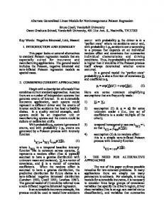
Example: Quadratic approximation of the log-likelihood Consider again the thumbtack example. The log-likelihood function is: l(θ) = y log θ + (n − y) log(1 − θ) + const
The score function is: l0 (θ) =
y n−y − , θ 1−θ
and the observed information: j(θ) =
y n−y + . θ2 (1 − θ)2
For n = 10, y = 3 and θb = 0.3 we obtain b = 47.6 j(θ)
The quadratic approximation is poor in this case. By increasing the sample size to n = 100, but still with θb = 0.3 the approximation is much better. Henrik Madsen Poul Thyregod (IMM-DTU)
Chapman & Hall
October 2010
11 / 32
Distribution of the ML estimator
0 0.2
0.4
0.6
0.8
1.0
-1 -2
Log-likelihood
-1 -2 0.0
True Approx.
-3
True Approx.
-3
Log-likelihood
0
18 The likelihood principle Example: Quadratic approximation of the log-likelihood
0.0
θ
0.2
0.4
0.6
0.8
1.0
θ
(a) n = 10, y = 3
(b) n = 100, y = 30
Figure 2.3: Quadratic approximation of the log-likelihood function.
Figure: Quadratic approximation of the log-likelihood function.
Example 2.7 (Quadratic approximation of the log-likelihood)
Henrik Madsen Poul Thyregod (IMM-DTU)
Chapman & Hall
October 2010
12 / 32
Model selection
Likelihood ratio tests
Methods for testing hypotheses using the likelihood function. The basic idea: determine the maximum likelihood estimates under both a null and alternative hypothesis. It is assumed that a sufficient model with θ ∈ Ω exists. Then consider some theory or assumption about the parameters H0 : θ ∈ Ω0 where Ω0 ⊂ Ω ; dim(Ω0 ) = r and dim(Ω) = k The purpose of the testing is to analyze whether the observations provide sufficient evidence to reject this theory or assumption. If not we accept the null hypothesis.
Henrik Madsen Poul Thyregod (IMM-DTU)
Chapman & Hall
October 2010
13 / 32
Model selection
Likelihood ratio tests
The evidence against H0 is measured by the p-value. The p-value is the probability under H0 of observing a value of the test statistic equal to or more extreme as the actually observed test statistic. Hence, a small p-value (say ≤ 0.05) leads to a strong evidence against H0 , and H0 is then said to be rejected. Likewise, we retain H0 unless there is a strong evidence against this hypothesis. Rejecting H0 given H0 is true is called a Type I error, while retaining H0 when the truth is actually H1 is called a Type II error.
Henrik Madsen Poul Thyregod (IMM-DTU)
Chapman & Hall
October 2010
14 / 32
Model selection
Likelihood ratio tests
Definition (Likelihood ratio) Consider the hypothesis H0 : θ ∈ Ω0 against the alternative H1 : θ ∈ Ω \ Ω0 (Ω0 ⊆ Ω), where dim(Ω0 ) = r and dim(Ω) = k. For given observations y1 , y2 , ..., yn the likelihood ratio is defined as λ(y) =
supθ∈Ω0 L(θ; y) supθ∈Ω L(θ; y)
If λ is small, then the data are seen to be more plausible under the alternative hypothesis than under the null hypothesis. Hence the hypothesis (H0 ) is rejected for small values of λ.
Henrik Madsen Poul Thyregod (IMM-DTU)
Chapman & Hall
October 2010
15 / 32
Model selection
Likelihood ratio tests It is sometimes possible to transform the likelihood ratio into a statistic, the exact distribution of which is known under H0 . This is for instance the case for the General Linear Model for Gaussian data. In most cases, however, we must use following important result regarding the asymptotic behavior. Theorem (Wilk’s Likelihood Ratio test) For λ(y), then under the null hypothesis H0 , the random variable −2 log λ(Y ) converges in law to a χ2 random variable with (k − r) degrees of freedom, i.e., −2 log λ(Y ) → χ2 (k − r) under H0 . Henrik Madsen Poul Thyregod (IMM-DTU)
Chapman & Hall
October 2010
16 / 32
Model selection
Null model and full model
The null model Ωnull = R (dim(Ωnull ) = 1), is a model with only one parameter.
The full model Ωfull = Rn (dim(Ωfull ) = n), is a model where the dimension is equal to the number of observations and hence the model fits each observation perfectly.
Henrik Madsen Poul Thyregod (IMM-DTU)
Chapman & Hall
October 2010
17 / 32
Model selection
The deviance
The deviance Let us introduce L0 = sup L(θ; y) and L = sup L(θ; y) then we notice θ∈Ω0
θ∈Ωfull
that −2 log λ(Y ) = −2(log L0 − log L) = 2(log L − log L0 ). The statistic D = −2 log λ(Y ) = 2(log L − log L0 ) is called the deviance.
Henrik Madsen Poul Thyregod (IMM-DTU)
Chapman & Hall
October 2010
18 / 32
Model selection
Hypothesis chains
Consider a chain of hypotheses specified by a sequence of parameter spaces R ⊆ ΩM . . . ⊂ Ω2 ⊂ Ω1 ⊂ Rn . For each parameter space Ωi we define a hypothesis Hi : θ ∈ Ω i with dim(Ωi ) < dim(Ωi−1 ).
Henrik Madsen Poul Thyregod (IMM-DTU)
Chapman & Hall
October 2010
19 / 32
Model selection
Partial likelihood ratio test
Definition (Partial likelihood ratio test) Assume that the hypothesis Hi allows the sub hypothesis Hi+1 ⊂ Hi . The partial likelihood ratio test for Hi+1 under Hi is the likelihood ratio test for the hypothesis Hi+1 under the assumption that the hypothesis Hi holds. The likelihood ratio test statistic for this partial test is λHi+1 |Hi (y) =
supθ∈Ωi+1 L(θ; y) supθ∈Ωi L(θ; y)
When Hi+1 holds, the distribution of λHi+1 |Hi (Y ) approaches a χ2 (f ) distribution with f = dim(Ωi ) − dim(Ωi+1 ).
Henrik Madsen Poul Thyregod (IMM-DTU)
Chapman & Hall
October 2010
20 / 32
Model selection
Partial tests Theorem (Partitioning into a sequence of partial tests) Consider a chain of hypotheses. Now, assume that H1 holds, and consider the minimal hypotheses HM : θ ∈ ΩM with the alternative H1 : θ ∈ Ω1 \ ΩM . The likelihood ratio test statistic λHM |H1 (y) for this hypothesis may be factorized into a chain of partial likelihood ratio test statistics λHi+1 |Hi (y) for Hi+1 given Hi , i = 1, . . . , M .
The partial tests ”corrects” for the effect of the parameters that are in the model at that particular stage When interpreting the test statistic corresponding to a particular stage in the hierarchy of models, one often says that there is ”controlled for”, or ”corrected for” the effect of the parameters that are in the model at that stage. Henrik Madsen Poul Thyregod (IMM-DTU)
Chapman & Hall
October 2010
21 / 32
Model selection
Two factor experiment 2.12
Successive testing in hypothesis chains
23
Length ∗ T hick
Length + T hick �Q � Q � Q � QQ � Length T hick QQ �� Q � Q � Q� ∅ Figure 2.6: Inclusion diagram corresponding two-factor experiment. In the Figure: Inclusion diagram corresponding to to a atwo-factor experiment. Theupper level we have used the same notation as used by the software R, i.e. Length∗Thick notation is the same as used by the software R, i.e. Length∗Thick denotes a denotes a two-factor model with interaction between the two factors. two-factor model with interaction between the two factors.
x Remark (The Henrik Madsen Poul Thyregod 2.8 (IMM-DTU)
partial Chapman tests &“corrects” for the effect Hall Octoberof 2010the 22 / 32
Model selection
Three factor 24experiment
The likelihood principle
A∗B∗C !aa !! aa ! ! aa ! aa !! A∗B+A∗C A∗B+B∗C A∗C +B∗C aa ! a ! aa aa!!! !! a! ! aa ! aa ! ! aa!! aa !! B∗C +A A∗B+C A∗C +B Q �\ �� � Q � � \ �� Q � Q� ��\ �Q �� � � � Q \ ��� Q � � Q \ A+B+C A∗B A∗C B∗C P QPP � � Q PP � Q � P � Q� PPP � �Q PP Q � � PP Q � PP � Q� A+B A+C B+C aa !aa ! aa!!! aa!!! !! aaa !!! aaa ! ! a! a A B C aa !! aa ! ! aa ! aa!!! ∅ Figure 2.7: Inclusion diagram corresponding to three-factor models. The notation Figure: Inclusion diagram corresponding to a athree-factor experiment. is the same as used by the software R, i.e. A∗B denotes two-factor model with between the two factors. Henrik Madsen Poul Thyregod interaction (IMM-DTU) Chapman & Hall
October 2010
23 / 32
Model selection
Strategies for variable selection in hypothesis chains Typically, one of the following principles for model selection is used: a) Forward selection: Start with a null model, add at each step the variable that would give the lowest p-value of the variable not yet included in the model. b) Backward selection: Start with a model containing all variables, variables are step by step deleted from the model. At each step, the variable with the largest p-value is deleted. c) Stepwise selection: This is a modification of the forward selection principle. Variables are added to the model step by step. In each step, the procedure also examines whether variables already in the model can be deleted. d) Best subset selection: For k = 1, 2, ... up to a user-specified limit, the procedure identifies a specified number of best models containing k variables. Henrik Madsen Poul Thyregod (IMM-DTU)
Chapman & Hall
October 2010
24 / 32
Model selection
Variable selection in hypothesis chains
In-sample methods for model selection The model complexity is evaluated using the same observations as those used for estimating the parameters of the model. The training data is used for evaluating the performance of the model. Any extra parameter will lead to a reduction of the loss function. In the in-sample case statistical tests are used to access the significance of extra parameters, and when the improvement is small in some sense the parameters are considered to be non-significant. The classical statistical approach.
Henrik Madsen Poul Thyregod (IMM-DTU)
Chapman & Hall
October 2010
25 / 32
Model selection
Variable selection in hypothesis chains
Statistical learning or data mining We have a data-rich situation such that only a part of the data is needed for model estimation and the rest can be used to test its performance. Seeking the generalized performance of a model which is defined as the expected performance on an independent set of observations. The expected performance can be evaluated as the expected value of the generalized loss function. The expected prediction error on an independent set of observations is called the test error or generalization error.
Henrik Madsen Poul Thyregod (IMM-DTU)
Chapman & Hall
October 2010
26 / 32
Model selection
Variable selection in hypothesis chains
In a data-rich situation, the performance can be evaluated by splitting the total set of observations in three parts: training set: used for estimating the parameters validation set: used for out-of-sample model selection test set: used for assessing the generalized performance, i.e. the performance on new data
A typical split of data is 50 pct for training and 25 pct for both validation and testing.
Henrik Madsen Poul Thyregod (IMM-DTU)
Chapman & Hall
October 2010
27 / 32
Model selection
26
The likelihood principle
Prediction error
Variable selection in hypothesis chains
Test set
Training set
Model complexity
Figure: A typical behavior of the (possibly generalized) training and test prediction error as a function of the model complexity.
Figure 2.8: A typical behavior of the (possibly generalized) training and test prediction error as a function of the model complexity
Henrik Madsen Poul Thyregod (IMM-DTU)
Chapman & Hall
October 2010
28 / 32
Dealing with nuisance parameters
Nuisance parameters
In many cases, the likelihood function is a function of many parameter but our interest focuses on the estimation on one or a subset of the parameters, with the others being considered as nuisance parameters Methods are needed to summarize the likelihood on a subset of the parameters by eliminating the nuisance parameters. Accounting for the extra uncertainty due to unknown nuisance parameters is an essential consideration, especially in small-sample cases.
Henrik Madsen Poul Thyregod (IMM-DTU)
Chapman & Hall
October 2010
29 / 32
Dealing with nuisance parameters
Profile likelihood
Definition (Profile likelihood) Assume that the statistical model for the observations Y1 , Y2 , . . . , Yn is given by the family of joint densities, θ = (τ, ζ) and τ denoting the parameter of interest. Then the profile likelihood function for τ is the function LP (τ ; y) = sup L((τ, ζ); y) ζ
where the maximization is performed at a fixed value of τ .
Henrik Madsen Poul Thyregod (IMM-DTU)
Chapman & Hall
October 2010
30 / 32
Dealing with nuisance parameters
Marginal likelihood Definition (Marginal likelihood) Assume that the statistical model for the observations Y1 , Y2 , . . . , Yn is given by the family of joint densities, θ = (τ, ζ) and τ denoting the parameter of interest. Let (U, V ) be a sufficient statistic for (τ, ζ) for which the factorization fU,V (u, v; (τ, ζ)) = fU (u; τ )fV |U =u (v; u, τ, ζ) holds. Provided that the likehood factor which corresponds to fV |U =u (·) can be neglected, inference about τ can be based on the marginal model for U with density fU (u; τ ). The corresponding likelihood function LM (τ ; u) = fU (u; τ ) is called the marginal likelihood function based on U . Henrik Madsen Poul Thyregod (IMM-DTU)
Chapman & Hall
October 2010
31 / 32
Dealing with nuisance parameters
Conditional likelihood Definition (Conditional likelihood) As above, assume that the statistical model for the observations Y1 , Y2 , . . . , Yn is given by the family of joint densities and θ = (τ, ζ) and τ denoting the parameter of interest. Let U = U (Y ) be a statistic such that the factorization fY (y; (τ, ζ)) = fU (u; τ, ζ)fY |U =u (y; u, τ ) holds. Provided that the likehood factor which corresponds to fU (·) can be neglected, inference about τ can be based on the conditional model for Y |U = u with density fY |U =u (·). The corresponding likelihood function LC (τ ) = LC (τ ; y|u) = fY |U =u (y; u, τ ) is called the conditional likelihood function based on conditioning on u. Henrik Madsen Poul Thyregod (IMM-DTU)
Chapman & Hall
October 2010
32 / 32