INTRODUCTION TO MATLAB SIMULINK - ENCON

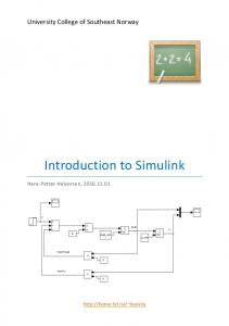
INTRODUCTION TO MATLAB 2:0 1:6

Pm = 0.8; E = 1.17; V = 1.0

1:2

X1 = 0.65; X2 = 1.8; X3 = 0.8; 0:8

eacfault(Pm, E, V, X1, X2, X3) 0:4

and

0

......................................... .............. .......... .......... ........ ........ ...... ...... ...... ...... ...... . . . . . ..... ..... . ..... . . . .... .... . . .... . . .... .... ............... ............................................... . .... . . . . . . . . . . . .... . . . . . ... ... ... ......... ......... .. .. ... ........ .... . . . . . . . . . . . . . . . . . . . . . . . . . . . . . . . . . . . . . . . . .... ... ... ... ... ... ... ... ... ... ........... .. .. .... . ....... . . . . . . . . . . . . . . . . .... . . . . . . . . . . . . . . . . . . . . . . . . . ... ... ... ... ... ... ... ... ... ... ... ... ... ... ........ .... . ..... . . . . . . . . . . . . . . . . . . .... . . . . . . . . . . . . . . . . . . . . . . . . . . . . . . . . . . . . . . . . . . . . . . . ... . ... ... ... ... ... ... ... ... ... ... ... ... ... ... ... ... ... ... ......... .. ..... ... . .... . . . . . . . . . . . . . . . . . . . . . . . . . . . . . . . . . . . . . . . . . . . . . . . . ... . . . . . . . . . . . . . . . . . . . . . . ... ... ... ... ... ... ... ... ... ... ... ... ... ... ... ... ... ... ... ... ... ... ..... .. ..... ... . ... . . . . . . . . . . . . . . . . . . . . . . . . . . . . . . . . . . . . . . . . . . . . . . . . . . . . . . . . . . ... ... ... ... ... ... ... ... ... ... ... ... ... ... ... ... ... ... ... ... ... ... ... ... ... ...... .. .. ..... ... . . . . . . . . . . . . . . . . . . . . . . . . . . . ... . . . . . . . . . . . . . . . . . . . . . . . . . . . . . . . . . . . . . . . . . . . . . . . . . . . . . . . . . . . . . . . . ... ... ... ... ... ... ... ... ... ... ... ... ... ... ... ... ... ... ... ... ... ... ... ... ... ... ... .... ... .. .. .... ... . . . . . . . . . . . . . . . . . . . . . . . . . . . . . . . . .. . . . . . . . . . . . . . . . . . . . . . . . . . . . . . . . . . . . .. ... ... ... ... ... ... ... ... ... ... ... ... ... ... ... ... ... ... ... ... ... ... ... ... ... ... ... ... ... ...... . . ... ....... ... ... ... ... ... ... ... ... ... ... ... ... ... ... ... ... ... ... ... ... ... ... ... ... ... ... ... ... ... ... ... ..... ..... . . . . . ... ... ... ... ... ... ... ... ... ... ... ... ... ... ... ... ... ... ... ... ... ... ... ... ... ... ... ... ... ... ... ... ...... ... . ... ....... .. . . . . . . . . . . . . . . . . . . . . . . . . . . . . . . . . . . . . . . . . . . . . . . . . . . . . . . . . . . . . . . . . . . . . . . . . ... ... ... ... ... ... ... ... ... ... ... ... ... ... ... ... ... ... ... ... ... ... ... ... ... ... ... ... ... ... ... ... ... ... ....... ..... .. ...................................................................................................................... . . . . . . . . . . . . . . . ................................................. . . . . . . . . . . . . . . . . . . . . . . . . . . . . . . . . . . . . . . . . . . . . . . . . . . . . . . . . . . . . . . . . . . . . . . . . . . . . . . . . . . . . . . . . . . . . . . . . . . . . ... . ...................... ... ... ....... ... ... ... ... ... ... ... ... ... ... ... ... ... ... ... ... ... ... ... ... ... ... ... ... ... ... ... ... ... ... ... ... ... ... ... ... ... ... ... ... ... ... ... ... ... ... ... ... ... ... ... .. . . . . . .... .. . ... . . . . . . . . . . . . . . . . . . . . . . . . . . . . . . . . . . . . . . . . . . . . . . . . . . . . .... . .. .. .. .. .. .. .. .. .. .. .. .. .. .. .. .. .. .. .. .. .. .. .. .. .. .. .. .. .. .. .. .. .. .. .. .. .. .. .. .. .. .. .. .. .. .. .. .. .. .. .. .. .. .. ..... .... .. .. .. .. .. .. .. .. .. .. .. .. .. .. .. .. .. .. .. .. .. .. .. .. .. .. .. .. .. .. .. .. .. .. .. .. .. .. .. .. .. .. .. .. .. .. .. .. .. .. .. .. .. .. ... ... ... .. . . . . . . . . . . . . . . . . . . . . . . . . . . . . . . . . . . . . . . . . . . . . . . . . . . . . . . . . . . . . . . . . . . . . . . . . . . . . . . . . . . . . . . . . . ... .. .. .. .. ... . . . .. ... . ... .. .. .. .. .. .. .. .. .. .. .. .. .. .. .. .. .. .. .. .. .. .. .. .. .. .. .. .. .. .. .. .. .. .. .. .. ..... ....... ..... ...... ..... ............ ............ ..... . ....... ..... .. .. .. .. .. .. .. .. .. .. .. .. .. .. .. .. .. .. .. .. .. .. .. .. .. .. .. .. .. .. .. .. .. ... ... ... ...... ..... . ......... ......................... .............. . . . . . . . . . . . . . . . . . . . . . . . . . . . . . . . . . . . . . . ... ........ . . . . . . . . . . . . . . . . . . . . . . . . . . . . . . . . . . . . . .... ... . . . . . . . . . . . . . . . . . . . . . . . . . . . . . . . . . . . . . . ............... . . ... ... ... ... ... ... ... ... ... ... ... ... ... ... ... ... ... ... ... ... ... ... ... ... ..................... .. . . . . . ............ .... ... ... ..... . . . . . . . . . . . . . . . . . . . . . . . . . . . . . . . . . . . . . . . . . . . . . . . . . . . . . . . . ... ... ... ... ... ... ... ... ... ... ... ... ... ... ... ... ... .............. ........... .. ... ... .. . . . ... ... ... ... ... ... ... ... ... ... ... ... ... .... . . . . . ......... . . . . . . . . . ... ... . . . . . . . . . . . ......... ... ... ... ... ... ... ... ... ... ... ............... .. . . ... .. .. . . ........ . . . . . . . . . . . . . . . . ... ... . . . . . . . . . . . . . . . ... ... ... ... ... ... ... ........ . .. . . ... .. . . ... ... ... ..... ........... ....... ........ . . . . . . . ... .. . .. ... .. ....... ...... ... . ............... ........ . . . . . . . ..... ....... . . ....... ..... . . . ......... . . . . . . . . . ....... ..... . . . .... ...... . . . . . . . . . . . .... . . . . . . . ....... .......... ... ........... .. . ....... ....... . . . . . . . . . . . ............ . . . ....... ... .. . ... . . ......... . . . . . . . ...... . . . ... . . . .. ... ... . . .

0

30

60

90

120

150

180

SIMULINK Pm

= 0:8

............. .... .............................. .... . ........... ........................ Step

+

............. ....... ... ....... .. ....... ... ....... ....... ... . . ......................... pi*60/5 ......................... .. ....... . ........ .... ...... ... ............. .............

!_

! 1

s

........................

Integ1

1

s

......... . . ....... . . ....... . . ....... . . ....... ....... ................... . ....... .. ... ... . 180/pi ... . . . ....... . . ....... . . . . . ....... . . . . . . . . . ........ . . . . . . . ..

Integ2

Sum

Pe

.. .. ... .. .. .. . . .. ...

n

.............................

1.4625*sin(u)

.............................

... ... ...........

ÆÆ

Æ .................. ........................

Rad. to Degree

Scope

................. ... ........ .

Fault cleared t

During fault

.............................

0.65*sin(u)

............................. ..... ....... .

Set the Switch Threshold at the value of fault clearing time

Hadi Saadat

INTRODUCTION TO MATLAB AND SIMULINK version v3.0

Hadi Saadat Professor of Electrical Engineering Milwaukee School of Engineering Milwaukee, Wisconsin

c 2000, Hadi Saadat. All rights reserved. Copyright Introduction to MATLAB and SIMULINK, and the accompanying m-files are distributed for the MSOE students. It may not be altered in any way, or be used as part of other documents.

CONTENTS

1 INTRODUCTION TO MATLAB 1.1 INSTALLING THE TEXT TOOLBOX . . . . . . . . . . . . 1.2 RUNNING MATLAB . . . . . . . . . . . . . . . . . . . . . . 1.3 VARIABLES . . . . . . . . . . . . . . . . . . . . . . . . . . 1.4 OUTPUT FORMAT . . . . . . . . . . . . . . . . . . . . . . 1.5 CHARACTER STRING . . . . . . . . . . . . . . . . . . . . 1.6 VECTOR OPERATIONS . . . . . . . . . . . . . . . . . . . . 1.7 ELEMENTARY MATRIX OPERATIONS . . . . . . . . . . . 1.7.1 UTILITY MATRICES . . . . . . . . . . . . . . . . . 1.7.2 EIGENVALUES . . . . . . . . . . . . . . . . . . . . 1.8 COMPLEX NUMBERS . . . . . . . . . . . . . . . . . . . . 1.9 POLYNOMIAL ROOTS AND CHARACTERISTIC POLYNOMIAL . . . . . . . . . . 1.9.1 PRODUCT AND DIVISION OF POLYNOMIALS . . 1.9.2 POLYNOMIAL CURVE FITTING . . . . . . . . . . 1.9.3 POLYNOMIAL EVALUATION . . . . . . . . . . . . 1.9.4 PARTIAL-FRACTION EXPANSION . . . . . . . . . 1.10 GRAPHICS . . . . . . . . . . . . . . . . . . . . . . . . . . . 1.11 GRAPHICS HARD COPY . . . . . . . . . . . . . . . . . . . 1.12 THREE-DIMENSIONAL PLOTS . . . . . . . . . . . . . . . 1.13 HANDLE GRAPHICS . . . . . . . . . . . . . . . . . . . . . 1.14 LOOPS AND LOGICAL STATEMENTS . . . . . . . . . . . 1.15 SIMULATION DIAGRAM . . . . . . . . . . . . . . . . . . . 1.16 INTRODUCTION TO SIMULINK . . . . . . . . . . . . . . 1.16.1 SIMULATION PARAMETERS AND SOLVER . . . 1.16.2 THE SIMULATION PARAMETERS DIALOG BOX . 1.16.3 BLOCK DIAGRAM CONSTRUCTION . . . . . . . 1.16.4 USING THE TO WORKSPACE BLOCK . . . . . . . 1.16.5 LINEAR STATE-SPACE MODEL FROM SIMULINK DIAGRAM . . . . . . .

. . . . . . . . . .

. . . . . . . . . .

. . . . . . . . . .

. . . . . . . . . .

1 2 2 4 4 7 7 10 12 12 13

. . . . . . . . . . . . . . . .

. . . . . . . . . . . . . . . .

. . . . . . . . . . . . . . . .

. . . . . . . . . . . . . . . .

15 16 17 18 18 19 21 27 30 30 36 38 39 40 41 47

. . . . 47 i

ii CONTENTS

1.16.6 SUBSYSTEMS AND MASKING . . . . . . . . . . . . . . . 49

CHAPTER

1 INTRODUCTION TO MATLAB

MATLAB, developed by Math Works Inc., is a software package for high performance numerical computation and visualization. The combination of analysis capabilities, flexibility, reliability, and powerful graphics makes MATLAB the premier software package for electrical engineers. MATLAB provides an interactive environment with hundreds of reliable and accurate built-in mathematical functions. These functions provide solutions to a broad range of mathematical problems including matrix algebra, complex arithmetic, linear systems, differential equations, signal processing, optimization, nonlinear systems, and many other types of scientific computations. The most important feature of MATLAB is its programming capability, which is very easy to learn and to use, and which allows user-developed functions. It also allows access to Fortran algorithms and C codes by means of external interfaces. There are several optional toolboxes written for special applications such as signal processing, control systems design, system identification, statistics, neural networks, fuzzy logic, symbolic computations, and others. MATLAB has been enhanced by the very powerful SIMULINK program. SIMULINK is a graphical mouse-driven program for the simulation of dynamic systems. SIMULINK enables students to simulate linear, as well as nonlinear, systems easily and efficiently. The following section describes the use of MATLAB and is designed to give a quick familiarization with some of the commands and capabilities of MATLAB. For a description of all other commands, MATLAB functions, and many other useful features, the reader is referred to the MATLAB User’s Guide. 1

2

1. INTRODUCTION TO MATLAB

1.1 INSTALLING THE TEXT TOOLBOX The software diskette included with the book contains all the developed functions and chapter examples. The file names for chapter examples begin with the letters ch. For example, the M-file for Example 2.4 is ch2ex04. Create a subdirectory, such as HS, where the MATLABR11 toolbox resides. Copy all the files on the diskette to the subdirectory MATLABR11 nTOOLBOXnHS. In the MATLAB 5.3 Command Window open the Path Browser by selecting Set Path from the File menu. Press to open the Add to Path window. Open the toolbox folder and double-click on the HS folder. Choose Add to Back option and click on Save Settings to save the new path permanently.

1.2 RUNNING MATLAB MATLAB supports almost every computational platform. MATLAB for WINDOWS is started by clicking on the MATLAB icon. The Command window is launched, and after some messages such as intro, demo, help help, info, and others, the prompt “ ” is displayed. The program is in an interactive command mode. Typing who or whos displays a list of variable names currently in memory. Also, the dir command lists all the files on the default directory. MATLAB has an on-line help facility, and its use is highly recommended. The command help provides a list of files, built-in functions and operators for which on-line help is available. The command

help function name will give information on the specified function as to its purpose and use. The command

help help will give information as to how to use the on-line help. MATLAB has a demonstration program that shows many of its features. The command demo brings up a menu of the available demonstrations. This will provide a presentation of the most important MATLAB facilities. Follow the instructions on the screen – it is worth trying. MATLAB 5.3 includes a Help Desk facility that provides access to on line help topics, documentation, getting started with MATLAB, online reference materials, MATLAB functions, real-time Workshop, and several toolboxes. The online documentation is available in HTML, via either Netscape Navigator or Microsoft Internet Explorer. The command helpdesk launches the Help Desk, or you can use the Help menu to bring up the Help Desk. If an expression with correct syntax is entered at the prompt in the Command window, it is processed immediately and the result is displayed on the screen. If an expression requires more than one line, the last character of the previous line must

1.2. RUNNING MATLAB

3

%

contain three dots “...”. Characters following the percent sign are ignored. The ( ) may be used anywhere in a program to add clarifying comments. This is especially helpful when creating a program. The command clear erases all variables in the Command window. MATLAB is also capable of executing sequences of commands that are stored in files, known as script files or M-files. Clicking on File, Open M-file, opens the Edit window. A program can be written and saved in ASCII format with a filename having extension .m in the directory where MATLAB runs. To run the program, click on the Command window and type the filename without the .m extension at the MATLAB command “”. You can view the text Edit window simultaneously with the Command window. That is, you can use the two windows to edit and debug a script file repeatedly and run it in the Command window without ever quitting MATLAB. In addition to the Command window and Edit window are the Graphic windows or Figure windows with grey (default) background. The plots created by the graphic commands appear in these windows. Another type of M-file is a function file. A function provides a convenient way to encapsulate some computation, which can then be used without worrying about its implementation. In contrast to the script file, a function file has a name following the word “function” at the beginning of the file. The filename must be the same as the “function” name. The first line of a function file must begin with the function statement having the following syntax

function [output arguments] = function name (input arguments)

The output argument(s) are variables returned. A function need not return a value. The input arguments are variables passed to the function. Variables generated in function files are local to the function. The use of global variables make defined variables common and accessible between the main script file and other function files. For example, the statement global R S T declares the variables R, S , and T to be global without the need for passing the variables through the input list. This statement goes before any executable statement in the script and function files that need to access the values of the global variables. Normally, while an M-file is executing, the commands of the file are not displayed on the screen. The command echo allows M-files to be viewed as they execute. echo off turns off the echoing of all script files. Typing what lists M-files and Mat-files in the default directory. MATLAB follows conventional Windows procedure. Information from the command screen can be printed by highlighting the desired text with the mouse and then choosing the print Selected ... from the File menu. If no text is highlighted the entire Command window is printed. Similarly, selecting print from the Figure window sends the selected graph to the printer. For a complete list and help on general purpose commands, type help general.

4


1.3 VARIABLES Expressions typed without a variable name are evaluated by MATLAB, and the result is stored and displayed by a variable called ans. The result of an expression can be assigned to a variable name for further use. Variable names can have as many as 19 characters (including letters and numbers). However, the first character of a variable name must be a letter. MATLAB is case-sensitive. Lower and uppercase letters represent two different variables. The command casesen makes MATLAB insensitive to the case. Variables in script files are global. The expressions are composed of operators and any of the available functions. For example, if the following expression is typed

x = exp(-0.2696*.2)*sin(2*pi*0.2)/(0.01*sqrt(3)*log(18)) the result is displayed on the screen as

x =

18.0001

and is assigned to x. If a variable name is not used, the result is assigned to the variable ans. For example, typing the expression

250/sin(pi/6) results in

ans =

500.0000

If the last character of a statement is a semicolon (;), the expression is executed, but the result is not displayed. However, the result is displayed upon entering the variable name. The command disp may be used to display a variable without printing its name. For example, disp(x) displays the value of the variable without printing its name. If x contains a text string, the string is displayed.

1.4 OUTPUT FORMAT While all computations in MATLAB are done in double precision, the default format prints results with five significant digits. The format of the displayed output can be controlled by the following commands.

1.4. OUTPUT FORMAT

MATLAB Command format format short format long format short e format long e format short g format long g format hex format + format bank format rat format compact format loose

5

Display Default. Same as format short Scaled fixed point format with 5 digits Scaled fixed point format with 15 digits Floating point format with 5 digits Floating point format with 15 digits Best of fixed or floating point with 5 digits Best of fixed or floating point with 15 digits Hexadecimal format The symbols +, - and blank are printed for positive, negative, and zero elements Fixed format for dollars and cents Approximation by ratio of small integers Suppress extra line feeds Puts the extra line feeds back in

For more flexibility in the output format, the command fprintf displays the result with a desired format on the screen or to a specified filename. The general form of this command is the following.

fprintf{fstr, A,...) writes the real elements of the variable or matrix A,... according to the specifications in the string argument of fstr. This string can contain format characters like ANCI C with certain exceptions and extensions. fprintf is ”vectorized” for the case when A is nonscalar. The format string is recycled through the elements of A (columnwise) until all the elements are used up. It is then recycled in a similar manner through any additional matrix arguments. The characters used in the format string of the commands fprintf are listed in the table below.

%e %E %f %s %u %i %x %X

Format codes scientific format, lower case e scientific format, upper case E decimal format string integer follows the type hexadecimal, lower case hexadecimal, upper case

nn nr nb nt ng 00 nn na

Control characters new line beginning of the line back space tab new page apostrophe back slash bell

A simple example of the fprintf is

fprintf('Area = %7.3f Square meters \n', pi*4.5^2) The results is

6


Area = 63.617 Square meters

%7 3

The : f prints a floating point number seven characters wide, with three digits after the decimal point. The sequence nn advances the output to the left margin on the next line. The following command displays a formatted table of the natural logarithmic for numbers 10, 20, 40, 60, and 80

x = [10; 20; 40; 60; 80]; y = [x, log(x)]; fprintf('\n Number Natural log\n') fprintf('%4i \t %8.3f\n',y') The result is

Number 10 20 40 60 80

Natural log 2.303 2.996 3.689 4.094 4.382

An M-file can prompt for input from the keyboard. The command input causes the computer to request data from the keyboard. For example, the command

R = input('Enter radius in meter ') displays the text string

Enter radius in meter and waits for a number to be entered. If a number, say 4.5 is entered, it is assigned to variable R and displayed as

R =

4.5000

The command keyboard placed in an M-file will stop the execution of the file and permit the user to examine and change variables in the file. Pressing cntrl-z terminates the keyboard mode and returns to the invoking file. Another useful command is diary A:filename. This command creates a file on drive A, and all output displayed on the screen is sent to that file. diary off turns off the diary. The contents of this file can be edited and used for merging with a word processor file. Finally, the command save filename can be used to save the expressions on the screen to a file named filename.mat, and the statement load filename can be used to load the file filename.mat. MATLAB has a useful collection of transcendental functions, such as exponential, logarithm, trigonometric, and hyperbolic functions. For a complete list and help on operators, type help ops, and for elementary math functions, type help elfun.

1.5. CHARACTER STRING

7

1.5 CHARACTER STRING A sequence of characters in single quotes is called a character string or text variable.

c ='Good' results in

c = Good A text variable can be augmented with more text variables, for example,

cs = [c, ' luck'] produces

cs =

Good luck

1.6 VECTOR OPERATIONS An n vector is a row or a column array of n numbers. In MATLAB, elements enclosed by brackets and separated by semicolons generate a column vector. For example, the statement

X = [ 2; -4; 8] results in

X =

2 -4 8

If elements are separated by blanks or commas, a row vector is produced. Elements may be any expression. The statement

R = [tan(pi/4) sqrt(9) -5] results in the output

R =

1.0000

3.0000

-5.0000

The transpose of a column vector results in a row vector, and vice versa. For example

Y=R'

8


will produce

Y =

1.0000 3.0000 -5.0000

MATLAB has two different types of arithmetic operations. Matrix arithmetic operations are defined by the rules of linear algebra. Array arithmetic operations are carried out element-by-element. The period character (.) distinguishes the array operations from the matrix operations. However, since the matrix and array operations are the same for addition and subtraction, the character pairs .+ and .- are not used. Vectors of the same size can be added or subtracted, where addition is performed componentwise. However, for multiplication, specific rules must be followed in order to obtain the correct resulting values. The operation of multiplying a vector X with a R scalar k (scalar multiplication) is performed componentwise. For example P produces the output

=5

P =

5.0000

15.0000

-25.0000

The inner product or the dotP product of two vectors X and Y denoted by hX; Y i is a scalar quantity defined by ni=1 xi yi . If X and Y are both column vectors defined above, the inner product is given by

S = X'*Y and results in

S =

-50

The operator (. performs element-by-element operation. For example, for the previously defined vectors, X and Y , the statement

E = X.*Y results in

E =

2 -12 -40

The operator .= performs element-by-element division. The two arrays must have the same size, unless one of them is a scalar. Array powers or element-by-element powers are denoted by ( .^). The trigonometric functions, and other elementary mathematical functions such as abs, sqrt, real, and log, also operate element by element. Various norms (measure of size) of a vector can be obtained. For example, the Euclidean norm is the square root of the inner product of the vector and itself. The command

1.6. VECTOR OPERATIONS

9

N = norm(X) produces the output

N =

9.1652

The angle between two vectors X and Y is defined by

cos = k h k k i k . The statement X;Y

X

Y

Theta = acos( X'*Y/(norm(X)*norm(Y)) ) results in the output

Theta =

2.7444

where Theta is in radians. The zero vector, also referred to as origin, is a vector with all components equal to zero. For example, to build a zero row vector of size 4, the following command

Z = zeros(1, 4) results in

Z =

0

0

0

0

The one vector is a vector with each component equal to one. To generate a one vector of size 4, use

I = ones(1, 4) The result is

I =

1

1

1

1

In MATLAB, the colon (:) can be used to generate a row vector. For example

x = 1:8 generates a row vector of integers from 1 to 8.

x =

1

2

3

4

5

6

7

8

For increments other than unity, the following command

z = 0 : pi/3 : pi results in

10 1. INTRODUCTION TO MATLAB

z =

0000

1.0472

2.0944

3.1416

For negative increments

x = 5 : -1:1 results in

x =

5

4

3

2

1

Alternatively, special vectors can be created, the command linspace(x, y, n) creates a vector with n elements that are spaced linearly between x and y . Similarly, the command logspace(x, y, n) creates a vector with n elements that are spaced in even logarithmic increments between x and y .

10

10

1.7 ELEMENTARY MATRIX OPERATIONS In MATLAB, a matrix is created with a rectangular array of numbers surrounded by brackets. The elements in each row are separated by blanks or commas. A semicolon must be used to indicate the end of a row. Matrix elements can be any MATLAB expression. The statement

A = [ 6 1 2; -1 8 3; 2 4 9] results in the output

A =

6 -1 2

1 8 4

2 3 9

If a semicolon is not used, each row must be entered in a separate line as shown below.

A = [ 6 -1 2

1 8 4

2 3 9]

The entire row or column of a matrix can be addressed by means of the symbol (:). For example

r3 = A(3, :) results in

r3 =

2

4

9

(: 2)

Similarly, the statement A ; addresses all elements of the second column in A. Matrices of the same dimension can be added or subtracted. Two matrices, A and B , can be multiplied together to form the product AB if they are conformable. Two symbols are used for nonsingular matrix division. AnB is equivalent to A 1 B , and A=B is equivalent to AB 1

1.7. ELEMENTARY MATRIX OPERATIONS

Example 1.1 For the matrix equation below, AX 2 4

4 2 2 10 4 6

11

= B , determine the vector X . 10 3 2 x 3 2 10 3 12 5 4 x 5 = 4 32 5 16 x 16 1 2 3

The following statements

A = [4 -2 -10; 2 10 -12; -4 -6 16]; B = [-10; 32; -16]; X = A\B result in the output

X =

2.0000 4.0000 1.0000

In addition to the built-in functions, numerous mathematical functions are available in the form of M-files. For the current list and their applications, see the MATLAB User’s Guide. Example 1.2 Use the inv function to determine the inverse of matrix A in Example 1.1 and then determine X . The following statements

A B C X

= = = =

[4 -2 -10; 2 10 -12; -4 -6 16]; [-10; 32; -16]; inv(A) C*B

result in the output

C =

X =

2.2000 0.4000 0.7000

2.3000 0.6000 0.8000

3.1000 0.7000 1.1000

2.0000 4.0000 1.0000

Example 1.3 Use the lu factorization function to express the matrix A of Example 1.2 as the product of upper and lower triangular matrices, A LU . Then find X from X U 1 L 1 B . Typing

=

=


A = [ 4 -2 -10; 2 10 -12; -4 -6 16 ] B = [-10; 32 -16]; [L,U] = lu(A) results in

L =

1.0000 0.5000 -1.0000

U =

4.0000 0 0

0 1.0000 -0.7273

0 0 1.0000

-2.0000 -10.0000 11.0000 -7.0000 0 0.9091

Now entering

X = inv(U)*inv(L)*B results in

X =

2.0000 4.0000 1.0000

Dimensioning is automatic in MATLAB. You can find the dimensions and rank of an existing matrix with the size and rank statements. For vectors, use the command length. 1.7.1

UTILITY MATRICES

There are many special utility matrices which are useful for matrix operations. A few examples are eye(m, n) zeros(m, n) ones(m, n) diag(x)

Generates an m-by-n identity matrix. Generates an m-by-n matrix of zeros. Generates an m-by-n matrix of ones. Produces a diagonal matrix with the elements of x on the diagonal line.

For a complete list and help on elementary matrices and matrix manipulation, type help elmat. There are many other special built-in matrices. For a complete list and help on specialized matrices, type help specmat. 1.7.2

EIGENVALUES

=

If A is an n-by-n matrix, the n numbers that satisfy Ax x are the eigenvalues of A. They are found using eig(A), which returns the eigenvalues in a column vector.

1.8. COMPLEX NUMBERS

13

Eigenvalues and eigenvectors can be obtained with a double assignment statement X; D eig A . The diagonal elements of D are the eigenvalues and the columns of X are the corresponding eigenvectors such that AX XD .

[

]= ( )

=

Example 1.4 Find the eigenvalues and the eigenvectors of the matrix A given by 2

A

=4

0 6 6

1 11 11

13 65 5

A = [ 0 1 -1; -6 -11 6; -6 -11 5]; [X,D] = eig(A) The eigenvalues and the eigenvectors are obtained as follows

X =

-0.7071 0.0000 -0.7071

0.2182 -0.0921 0.4364 -0.5523 0.8729 -0.8285

D =

-1 0 0

0 -2 0

0 0 -3

1.8 COMPLEX NUMBERS All the MATLAB operators are available for complex operations. The imagp isarithmetic predefined by two variables i and j . In a program, if other values inary unit are assigned to i and j , they must be redefined as imaginary units, or other characters can be defined for the imaginary unit.

1

j = sqrt(-1)

or i = sqrt(-1)

Once the complex unit has been defined, complex numbers can be generated. Example 1.5 Evaluate the following function V and g : j :

= 0 02 + 1 5

= Zc cosh g +sinh g=Zc, where Zc = 200+ j 300

i = sqrt(-1); Zc = 200 + 300*i; g = 0.02 + 1.5*i; v = Zc *cosh(g) + sinh(g)/Zc results in the output

v =

8.1672 + 25.2172i

It is important to note that, when complex numbers are entered as matrix elements within brackets, we avoid any blank spaces. If spaces are provided around the complex number sign, it represents two separate numbers.


Example 1.6 In the circuit shown in Figure 1.1, determine the node voltages V1 and V2 and the power delivered by each source.

"

30 + j 40A

V1 .... .... .. ... ... ..... .......... ..... ... . . . ........ ..... .. .......... ... ... .. .... ..... . ......... .. ......... .. .....

y12

= 0:35

12

j :

.................................... ... ... ... ... ...... ....... ....... ....... ........................... ... ... ... .. ... ... ... ...

= 1 15 j 0:8

V2 . . . . . . . . . . . ... . . ..... .......... ..... ... . . . ....... ..... ...... .. .. ... . . . . . . . . . . .... . .. . ......... .. ......... .. .....

= 0 55 j 0:4

y10 :

y20 :

20 + 15 " j

A

FIGURE 1.1 Circuit for Example 1.6.

Kirchhoff’s current law results in the following matrix node equation.

35 + j 1:2 V = 30 + j 40 0:9 j 1:6 V 20 + j 15 and the complex power of each source is given by S = V I . The following program

1:5 j 2:0 :35 + j 1:2

:

1 2

is written to yield solutions to V1 ,V2 and S using MATLAB.

j=sqrt(-1) % Defining j I=[30+j*40; 20+j*15] % Column of node current phasors Y=[1.5-j*2 -.35+j*1.2; -.35+j*1.2 .9-j*1.6] % Complex admittance matrix Y disp('The solution is') V=inv(Y)*I % Node voltage solution S=V.*conj(I) % complex power at nodes result in

The solution is V = 3.5902 + 35.0928i 6.0155 + 36.2212i S =

1511.4 + 909.2i 663.6 + 634.2i

In MATLAB, the conversion between polar and rectangular forms makes use of the following functions:

1.9. POLYNOMIAL ROOTS AND CHARACTERISTIC POLYNOMIAL

Operation z

= a + bi or z = a + j b

z

= M exp(j )

real(z ) imag(z ) abs(z ) angle(z ) conj(z )

15

Description Rectangular from Returns real part of z Returns imaginary part of z Absolute value of z Phase angle of z Conjugate of z converts M 6 to rectangular form

The prime (0 ) transposes a real matrix; but for complex matrices, the symbol (.0 ) must be used to find the transpose.

1.9 POLYNOMIAL ROOTS AND CHARACTERISTIC POLYNOMIAL If p is a row vector containing the coefficients of a polynomial, roots(p) returns a column vector whose elements are the roots of the polynomial. If r is a column vector containing the roots of a polynomial, poly(r) returns a row vector whose elements are the coefficients of the polynomial. Example 1.7 Find the roots of the following polynomial. s6

+ 9s + 31:25s + 61:25s + 67:75s + 14:75s + 15 5

4

3

2

The polynomial coefficients are entered in a row vector in descending powers. The roots are found using roots.

p = [ 1 9 31.25 61.25 67.75 14.75 15 ] r = roots(p) The polynomial roots are obtained in column vector

r =

-4.0000 -3.0000 -1.0000 -1.0000 0.0000 0.0000

Example 1.8

+ + -

2.0000i 2.0000i 0.5000i 0.5000i

1 2 3 4

, , j . Determine the polynomial equation. The roots of a polynomial are Complex numbers may be entered using function i or j . The roots are then entered in a column vector. The polynomial equation is obtained using poly as follows


i = sqrt(-1) r = [-1 -2 -3+4*i -3-4*i ] p = poly(r) The coefficients of the polynomial equation are obtained in a row vector.

p =

1 9 45 87 50

Therefore, the polynomial equation is s4

+ 9s + 45s + 87s + 50 = 0 3

2

Example 1.9 Determine the roots of the characteristic equation of the following matrix. 2

A

=4

0 6 6

1 11 11

13 65 5

The characteristic equation of the matrix is found by poly, and the roots of this equation are found by roots.

A = [ 0 1 -1; -6 -11 6; -6 -11 5]; p = poly(A) r = roots(p) The result is as follows

p =

1.0000 6.0000 11.0000 6.0000 r = -3.0000 -2.0000 -1.0000 The roots of the characteristic equation are the same as the eigenvalues of matrix A. Thus, in place of the poly and roots function, we may use

r = eig(A) 1.9.1

PRODUCT AND DIVISION OF POLYNOMIALS

The product of polynomials is the convolution of the coefficients. The division of polynomials is obtained by using the deconvolution command.

1.9. POLYNOMIAL ROOTS AND CHARACTERISTIC POLYNOMIAL

17

Example 1.10 (a) Given A (b) Given Z

= s + 7s + 12, and B = s + 9, find C = AB . = s + 9s + 37s + 81s + 52, and Y = s + 4s + 13, find X = 2

2

4

3

2

2

Z Y

.

The commands

A = C = Z = [X,

[1 7 12]; B = [1 0 9]; conv(A, B) [1 9 37 81 52]; Y = [1 4 r] = deconv(Z, Y)

13];

result in

C = X = r =

1.9.2

1

7

21

1 5

4

0 0

0

63

108

POLYNOMIAL CURVE FITTING

In general, a polynomial fit to data in vector x and y is a function p of the form

( ) = c x + c x + + c The degree is d, and the number of coefficients is n = d +1. Given a set of points p x

1

d

2

d

1

n

in vectors x and y , polyfit(x, y, d) returns the coefficients of dth order polynomial in descending powers of x. Example 1.11 Find a polynomial of degree 3 to fit the following data x y

0 1

1 7

2 23

4 109

6 307

10 1231

x = [ 0 1 2 4 6 10]; y = [ 1 7 23 109 307 1231]; c = polyfit(x,y,3) The coefficients of a third degree polynomial are found as follows

c = i.e., y

1.0000

2.0000

= x + 2x + 3x + 1. 3

2

3.0000

1.0000


1.9.3

POLYNOMIAL EVALUATION

If c is a vector whose elements are the coefficients of a polynomial in descending powers, the polyval(c, x) is the value of the polynomial evaluated at x. For example, to evaluate the above polynomial at points 0, 1, 2, 3, and 4, use the commands

c = [1 2 3 1]; x = 0:1:4; y = polyval(c, x) which result in

y =

1.9.4

7

23

55

109

PARTIAL-FRACTION EXPANSION

[r, p, k] = residue[b, a] finds the residues, poles, and direct terms of a partial fraction expansion of the ratio of two polynomials

( ) = b s +b ( ) a s +a

P s Q s

m

n

m n

m n

1s 1s

1

n

+ +b s + b + + a s +a

1

m

1

1

0

0

Vectors b and a specify the coefficients of the polynomials in descending powers of s. The residues are returned in column vector r, the pole locations in column vector p, and the direct terms in row vector k. Example 1.12 Determine the partial fraction expansion for

( ) = s 2+s s++9s4+s +1 4

F s

b = [ 2 0 9 1]; a = [ 1 1 4 4]; [r,p,k] = residue(b,a) The result is as follows

r =

p =

K =

0.0000 0.0000 -2.0000

-0.2500i +0.2500i

0.0000 0.0000 -1.0000

+2.0000i -2.0000i

2.0000

3

3

2

1.10. GRAPHICS

19

Therefore the partial fraction expansion is

2 + s +21 + sj 0+:25j 2 + s j 0:j252 = 2 + s +21 + s 1+ 4 2

[b, a] = residue(r, p, K) converts the partial fraction expansion back to the polynomial P s =Q s . For a complete list and help on matrix analysis, linear equations, eigenvalues, and matrix functions, type help matfun.

() ()

1.10 GRAPHICS MATLAB can create high-resolution, publication-quality 2-D, 3-D, linear, semilog, log, polar, bar chart and contour plots on plotters, dot-matrix printers, and laser printers. Some of the 2-D graph types are plot, loglog, semilogx, semi -logy, polar, and bar. The syntax for the above plots includes the following optional symbols and colors. COLOR SPECIFICATION Long name Short name black k blue b cyan c green g magenta m red r white w yellow y

LINE STYLE-OPTION Style Symbol solid – dashed -dotted : dash-dot -. point . circle o x-mark x plus + star *

Some of the Specialized 2-D plots are listed below: area bar barh comet ezplot ezpolar feather fill fplot hist pareto pie plotmatrix stem stairs

Filled area plot Bar graph Horizontal bar graph Comet-like trajectory Easy to use function plotter Easy to use polar coordinate plotter Feather plot Filled 2-D polygons Plot function Histogram Pareto chart Pie chart Scatter plot matrix Discrete sequence or ”stem” plot Stairstep plot


You have three options for plotting multiple curves on the same graph. For example,

plot(x1, y1,'r', x2, y2, '+b', x3, y3, '--') plots (x1, y1) with a solid red line, (x2, y2) with a blue + mark, and (x3, y3) with a dashed line. If X and Y are matrices of the same size, plot(X, Y) will plot the columns of Y versus the column of X. Alternatively, the hold command can be used to place new plots on the previous graph. hold on holds the current plot and all axes properties; subsequent plot commands are added to the existing graph. hold off returns to the default mode whereby a new plot command replaces the previous plot. hold, by itself, toggles the hold state. Another way for plotting multiple curves on the same graph is the use of the line command. For example, if a graph is generated by the command plot(x1, y1), then the commands

line(x2, y2, '+b') line(x3, y3, '--') Add curve (x2, y2) with a blue + mark, and (x2, y2) with a dashed line to the existing graph generated by the previous plot command. Multiple figure windows can be created by the figure command. figure, by itself, opens a new figure window, and returns the next available figure number, known as the figure handle. figure(h) makes the figure with handle h the current figure for subsequent plotting commands. Plots may be annotated with title, x y labels and grid. The command grid adds a grid to the graph. The commands title(’Graph title ’) titles the plot, and xlabel(’x-axis label ’), ylabel(’y-axis label ’) label the plot with the specified string argument. The command text(x-coordinate, y-coordinate, ’text’) can be used for placing text on the graph, where the coordinate values are taken from the current plot. For example, the statement

text(3.5, 1.5, 'Voltage') will write Voltage at point (3.5, 1.5) in the current plot. Alternatively, you can use the gtext(’text’) command for interactive labeling. Using this command after a plot provides a crosshair in the Figure window and lets the user specify the location of the text by clicking the mouse at the desired location. Finally, the command legend(string1, string2, string3, ...) may be used to place a legend on the current plot using the specified strings as labels. This command has many optional arguments. For example, legend( linetype1, string1, linetype2, string2, linetype3, string3, ...) specifies the line types/color for each label at a suitable location. However, you can move the legend to a desired location with the mouse. legend off removes the legend from the current axes. MATLAB provides automatic scaling. The command axis([x min. x max. y min. y max.]) enforces the manual scaling. For example

axis([-10

40

-60 60])

1.11. GRAPHICS HARD COPY

10

21

60

produces an x-axis scale from to 40 and a y -axis scale from to 60. Typing axis again or axis(’auto’) resumes auto scaling. Also, the aspect ratio of the plot can be made equal to one with the command axis(’square’). With a square aspect ratio, a line with slope 1 is at a true 45 degree angle. axis(’equal’) will make the x- and y -axis scaling factor and tic mark increments the same. For a complete list and help on general purpose graphic functions, and two- and three-dimensional graphics, see help graphics, help plotxy, and help plotxyz. There are many other specialized commands for two-dimensional plotting. Among the most useful are the semilogx and semilogy, which produce a plot with an x-axis log scale and a y -axis log scale. An interesting graphic command is the comet plot. The command comet(x, y) plots the data in vectors x and y with a comet moving through the data points, and you can see the curve as it is being plotted. For a complete list and help on general purpose graphic functions and two-dimensional graphics, see help graphics and help plotxy.

1.11 GRAPHICS HARD COPY The easiest way to obtain hard-copy printout is to make use of the Windows built-in facilities. In the Figure window, you can pull down the file menu and click on the Print command to send the current graph directly to the printer. You can also import a graph to your favorite word processor. To do this, select Copy options from the Edit pull-down menu, and check mark the Invert background option in the dialog box to invert the background. Then, use Copy command to copy the graph into the clipboard. Launch your word processor and use the Paste command to import the graph. Some word processors may not provide the extensive support of the Windows graphics and the captured graph may be corrupted in color. To eliminate this problem use the command

system dependent(14, 'on') which sets the metafile rendering to the lowest common denominator. To set the metafile rendering to normal, use

system dependent(14, 'off') In addition MATLAB provides a function called print that can be used to produce high resolution graphic files. For example,

print -dhpgl [filename] saves the graph under the specified filename with extension hgl. This file may be processed with an HPGL- compatible plotter. Similarly, the command

print -dilll [filename]


produces a graphic file compatible with the Adobe Illustrator’88. Another print option allows you to save and reload a figure. The command

print -dmfile [ filename ] produces a MAT file and M-file to reproduce the figure again. In the Figure window, from the File pull-down menu you can use Save As... to save the figure with extension fig. This file can be opened in the Figure window again. Also, from the File pull-down menu you can use Expert... to save the graph in several different format, such as: emf, bmp, eps, ai, jpg, tiff, png, pcx, pbm, pgm, and ppm extensions. Example 1.13 Create a linear X -Y plot for the following variables. x y

0 10

0.5 10

1.0 16

1.5 24

2.0 30

2.5 38

3.0 52

3.5 68

4.0 82

4.5 96

5.0 123

For a small amount of data, you can type in data explicitly using brackets.

x = [ 0 0.5 1.0 1.5 2.0 2.5 3.0 3.5 4.0 4.5 5.0]; y = [10 10 16 24 30 38 52 68 82 96 123]; plot(x, y), grid xlabel('x'), ylabel('y'), title('A simple plot example') plot(x, y) produces a linear plot of y versus x on the screen, as shown in Figure 1.2. For large amounts of data, use the text editor to create a file with extension m. Typing the filename creates your data in the workspace. Example 1.14 Fit a polynomial of order 2 to the data in Example 1.13. Plot the given data point with symbol x, and the fitted curve with a solid line. Place a boxed legend on the graph. The command p = polyfit(x, y, 2) is used to find the coefficients of a polynomial of degree 2 that fits the data, and the command yc = polyval(p, x) is used to evaluate the polynomial at all values in x. We use the following command.

x = [ 0 0.5 1.0 1.5 2.0 2.5 3.0 3.5 4.0 4.5 5.0]; y = [10 10 16 24 30 38 52 68 82 96 123]; p = polyfit(x, y, 2) % finds the coefficients of a polynomial % of degree 2 that fits the data yc = polyval(p, x);%polynomial is evaluated at all points in x plot(x, y,'x', x, yc)%plots data with x and fitted polynomial xlabel('x'), ylabel('y'), grid title('Polynomial curve fitting') legend('Actual data', 'Fitted polynomial', 4)

23


A simple plot example 140 120 100

y

80 60 40 20 0

0

1

2

3

4

5

x FIGURE 1.2 Example of -

X Y plot.

The result is the array of coefficients of the polynomial of degree 2, and is

p =

4.0232

2.0107

9.6783

4 0 + 2 0 + 9 68

Thus, the parabola : x2 : x : is found that fits the given data in the least-square sense. The plots are shown in Figure 1.3. Example 1.15

= 1+

sin(8

2)

e 2t t = from 0 to 3 seconds. Find the time corPlot function y responding to the peak value of the function and the peak value. The graph is to be labeled, titled, and have grid lines displayed.

Remember to use .* for the element-by-element multiplication of the two terms in the given equation. The command [cp, k] = max(c) returns the peak value and the index k corresponding to the peak time. We use the following commands.

t=0:.005:3; c = 1+ exp(-2*t).*sin(8*t - pi/2); [cp, k] = max(c) % cp is the maximum value of c at interval k tp = t(k) % tp is the peak time plot(t, c), xlabel(' t - sec'), ylabel('c'), grid title('Damped sine curve') text(0.6, 1.4, ['cp =',num2str(cp)])%Text in quote & the value % of cp are printed at the specified location text(0.6, 1.3, ['tp = ',num2str(tp)])


Polynomial curve fitting 140 120 100

y

80 60 40 20 0

Actual data Fitted polynomial 0

1

2

3

4

5

x FIGURE 1.3 Fitting a parabola to the data in Example 1.13.

The result is

cp = k = tp =

1.4702 73 0.3600

and the plot is shown in Figure 1.4. An interactive way to find the data points on the curve is by using the ginput command. Entering [x, y] = ginput will put a crosshair on the graph. Position the crosshair at the desired location on the curve, and click the mouse. You can repeat this procedure for extracting coordinates for as many points as required. When the return key is pressed, the input is terminated and the extracted data is printed on the command menu. For example, to find the peak value and the peak time for the function in Example 1.15, try

[tp, cp] = ginput A crosshair will appear. Move the crosshair to the peak position, and click the mouse. Press the return key to get

cp = tp =

1.47 0.36

25


Damped sine curve 1.5 cp = 1.4702 tp = 0.36

c

1

0.5

0

0

0.5

1

1.5 t, sec

2

2.5

3

FIGURE 1.4 Graph of Example 1.15.

subplot splits the Figure window into multiple portions, in order to show several plots at the same time. The statement subplot(m, n, p) breaks the Figure window into an mby-n box and uses the pth box for the subsequent plot. Thus, the command subplot(2, 2, 3), plot(x,y) divides the Figure window into four subwindows and plots y versus x in the third subwindow, which is the first subwindow in the second row. The command subplot(111) returns to the default Figure window. This is demonstrated in the next example. Example 1.16 Divide the Figure window into four partitions, and plot the following functions for !t from to in steps of : .

0 3

0 05

= 120sin !t and i = 100sin(!t

4) versus !t on the upper left

1. Plot v portion.

=

= vi on the upper right portion. 3. Given F = 3:0, plot f = F sin !t, F = F sin(!t 2=3), and F = F sin(!t 4=3) versus !t on the lower left portion. 4. For f = 3F , construct a circle of radius f on the lower right portion. 2. Plot p

m

a

m

m

b

c

m

R

m

wt = 0: 0.05: 3*pi; v=120*sin(wt); i = 100*sin(wt - pi/4);

R

%Sinusoidal voltage %Sinusoidal current


Voltage & current

Power

150

15000

100 10000 50 0

5000

−50 0 −100 −150

0

5 ωt, radians 3−phase mmf

10

3

−5000

0

5 ωt, radians Rotating mmf

10

0

5

5

2 1 0

0

−1 −2 −3

0

5 ωt, radians

10

−5 −5

FIGURE 1.5 Subplot demonstration.

p = v.*i; %Instantaneous power subplot(2, 2, 1), plot(wt, v, wt, i); %Plot of v & i versus wt title('Voltage & current'), xlabel('\omegat, radians'); subplot(2, 2, 2), plot(wt, p); % Instantaneous power vs. wt title('Power'), xlabel(' \omegat, radians ') Fm=3.0; fa = Fm*sin(wt); % Three-phase mmf's fa, fb, fc fb = Fm*sin(wt - 2*pi/3); fc = Fm*sin(wt - 4*pi/3); subplot(2, 2, 3), plot(wt, fa, wt, fb, wt, fc) title('3-phase mmf'), xlabel(' \omegat, radians ') fR = 3/2*Fm; subplot(2, 2, 4), plot(-fR*cos(wt), fR*sin(wt)) title('Rotating mmf'), subplot(111) Example 1.16 results are shown in Figure 1.5.

1.12. THREE-DIMENSIONAL PLOTS

27

1.12 THREE-DIMENSIONAL PLOTS MATLAB provides extensive facilities for visualization of three-dimensional data. The most common are plots of curves in a three-dimensional space, mesh plots, surface plots, and contour plots. The command plot3(x, y, z , ’style option’) produces a curve in the three-dimensional space. The viewing angle may be specified by the command view(azimuth, elevation). The arguments azimuth, and elevation specifies the horizontal and vertical rotation in degrees, respectively. The title, xlabel, ylabel, etc., may be used for three-dimensional plots. The mesh and surf commands have several optional arguments and are used for plotting meshes and surfaces. The contour(z) command creates a contour plot of matrix z, treating the values in z as heights above the plane. The statement mesh(z) creates a three-dimensional plot of the elements in matrix z. A mesh surface is defined by the z coordinates of points above a rectangular grid in the x-y plane. The plot is formed by joining adjacent points with straight lines. meshgrid transforms the domain specified by vector x and y into arrays X and Y. For a complete list and help on general purpose Graphic functions and three-dimensional graphics, see help graphics and help plotxyz. Also type demo to open the MATLAB Expo Menu Map and visit MATLAB. Select and observe the demos in the Visualization section. Following is a list of elementary 3-D plots and some specialized 3-D graphs. plot3 mesh surf fill3 comet3 ezgraph3 ezmesh ezmeshc ezplot3 ezsurf ezsurfc meshc meshz scatter3 stem3 surfc trisurf trimesh cylinder sphere

Plot lines and points in 3-D space 3-D mesh surface 3-D colored surface Filled 3-D polygons 3-D comet-like trajectories General purpose surface plotter Easy to use 3-D mesh plotter Easy to use combination mesh/contour plotter Easy to use 3-D parametric curve plotter Easy to use 3-D colored surface plotter Easy to use combination surf/contour plotter Combination mesh/contour plot 3-D mesh with curtain 3-D scatter plot 3-D stem plot Combination surf/contour plot Triangular surface plot Triangular mesh plot Generate cylinder Generate sphere

Example 1.17 ch1ex17.m Few examples of 3-D plots and mesh plots are given in Figure 1.6.


Plot of a parametric space curve x(t) = e−0.03t cos t, y(t) =e−0.03t sin t, z(t)=t t= 0:0.1:16*pi; x=exp(−0.03*t).*cos(t); y=exp(−0.03*t).*sin(t); z=t; plot3(x, y, z), axis off

2

2 0.5

−(x +y )

Plot of function z=sinx cosy e using mesh

t = −4:0.3:4; [x,y] = meshgrid(t,t); z = sin(x).*cos(y).*exp(−(x.^2+y.^2).^0.5); mesh(x,y,z), axis off Plot of function z=−0.1/(x2+y2+1) using meshz x= −3:0.3:3; y=x; [x, y]=meshgrid(x,y); z=−0.1./(x.^2+y.^2+.1); meshz(z) , axis off view(−35, 60)

Discrete plot of x=t, y=t cost, z=e0.1t using stem3 t=0:.2:20; x=t; y=t.*cos(t); z=exp(0.1*t); stem3(x,y,z), axis off

1.12. THREE-DIMENSIONAL PLOTS

29

Cylindrical surface created by p=3+sin t using cylinder function t=0:pi/5:6*pi; p=3+sin(t); cylinder(p), axis off

Plot of a unit sphere and a scaled sphere using sphere function [x,y,z]=sphere(24); subplot(2,2,2), surf(x−2, y−2, z−1); hold on surf(2*x, 2*y,2*z); axis off

Cartezian plot of Bessel function J0[x2+y2]1/2 −12