INTRODUCTION TO MATHCAD - ENCON

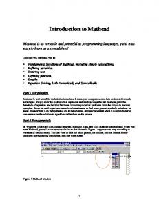
INTRODUCTION TO MATHCAD Mathcad is a program that does calculations, graphing, solving of equations, . . .

BASIC CALCULATIONS Open up the Arithmetic Palette by double clicking on the calculator icon in the Math Palette. If the Math Palette is not on your desktop then open it from the View Menu. EXAMPLE 1 - Simple Calculating 2 + 3∗ 5 = 1. The square root symbol is on the arithmetic palette 2. When you type the equal sign Mathcad will display the answer just like a regular calculator EXAMPLE 2 - Variables x := 5 y := x + 3 y= 1. Press the return after entering each line 2. The symbol := is on the Arithmetic Palette. It tells Mathcad to assign the value 5 to the variable x in the first line and x+3 to y in the second line 3. Typing y and then a "regular" equal sign on the keyboard tells Mathcad to display the value of y 4. If you change the value of x then the value of y will change 5. The placement of equations matters. The equation for y cannot come before you tell Mathcad the value of x. If you do something Mathcad doesn't like then the corresponding equation or variable will turn red. EXAMPLE 3 - Range Variables I n := 2, 3 .. 5 2*n = 1. The first line tells Mathcad that a. The first value of n = 2 b. The second value of n = 3 c. The difference between consecutive values of n is 3-2 = 1 d. The last value of n = 5 2. The symbol .. is on the Arithmetic Palette as m..n 3. When you type 2*n = Mathcad will generate a table of numbers - one for each value of n EXAMPLE 4 - Range Variables II a := 1, 1.1 .. 1.3 2*a = 1. The first line tells Mathcad that a. The first value of a = 1 b. The second value of a = 1.1 c. The difference between consecutive values of a is 1.1-1 = 0.1 d. The last value of a = 1.3 2. When you type 2*a = Mathcad will generate a table of numbers - one for each value of a 1

EXAMPLE 5 - Functions x := 0, 0.1 . . 0.5 y(x) := 2*x y(x) = 1. Mathcad evaluates the function y(x) for every value of x 2. Note that Mathcad won't accept y := 2*x when x is a range variable EXAMPLE 6 - Subscripted Variables n := 0, 1 . . 5 yn := 2*n yn = 1. The subscripted variable is from the Arithmetic Palette 2. The subscripts n must be positive integers with n ≥ 0 EXAMPLE 7 - Summations I 3

y:= ∑ n2 n= 0

y= 1. The summation sign is from the Calculus Palette EXAMPLE 8 - Summations II a := 0, 1 . . 3 3

y(a): = ∑ a ∗n 2 n=0

y(a) = 1. The summation will be calculated for each value of a EXAMPLE 9 - Vectors and Matrices I 1 X := 3 5 Y := 2*X Y= 1. Create the 3x1 vector by first clicking on the the icon in the upper left hand corner of the Vector and Matrix Palette and then entering the number of rows and columns. 2. Matrices (arrays) are particularly nice for storing data points

2

EXAMPLE 10 - Vectors and Matrices II 1 X := 3 5 a := 2*X0 b := 3*X1 c := 4*X2 a= b=

c=

1. The elements in the vector X are subscripted variables as follows X0 = 1 X1 = 3 X2 = 5 with subscripts n ≥ 0 EXAMPLE 11 - Complex Numbers z := i (1 + i) real := Re (z) imaginary := Im (z) r := |z| θ := arg(z) 1. The imaginary number i (our j) is from the Arithmetic Palette 2. The absolute value or magnitude operator | | is from the Arithmetic Palette EXAMPLE 12 - Phasors and Transfer Functions ω := 1000 Vs:= 2∗ e j∗1.2 G( ): =

1000 j ∗ + 1000

Vo(ω) := G(ω)*Vs |Vo(ω)| =

arg (Vo(ω)) =

1. ω is on the palette of Greek symbols 2. Note that we write G(ω) and Vo(ω) as functions of ω (not jω) EXAMPLE 13 - Integration 0.001

a:= ∫0 2 ∗ t ∗ sin(t)dt

TOL : = 0.00001

a= 1. The integral sign is from the Calculus Palette 2. The accuracy of the integral can in general be improved by making TOL smaller. Note that the nominal value of TOL is 0.001 as shown in options under the Math Menu. 3

EXAMPLE 14 - The Sinc Function x := -0.5, -0.4 . . 0.5 1 if x = 0 sinc(x): = sin(π ∗ x) otherwise π∗ x sinc (x) = 1. We have to tell Mathcad the value of the sinc function at x = 0 because when x = 0 the denominator of the function is equal to zero 2. In the equation for sinc(x) a. The vertical line is obtained by clicking on add line in the Programming Palette b. if and otherwise are from the Programming Palette c. The bold equal sign in the equation x = 0 is from the Evaluation and Boolean Palette EXAMPLE 15 - Fourier Series of a Sawtooth k := 1, 2 . . 5 T := 4

o

=

2π T

x(t) := 3*t ao : =

1 T x(t)dt T ∫0

ak :=

2 T x(t)cos( k ∗ T ∫0

ck :=

(ak )

2

+ (bk )

co := ao ∗ t )dt

o

2 k

bk :=

2 T x(t)sin (k ∗ T ∫0

o

∗t ) dt

: = angle(ak , − bk )

1. Use angle instead of atan because atan is only defined in the range -π/2 to π/2 EXAMPLE 16 - Difference Equations n := 0, 1 . . 5 y(n):=

0 0.5 ∗ y(n − 1) + 1

if n = -1 otherwise

y(n) = 1. We had to use this conditional statement for y(n) because Mathcad won't let us simply define y(-1) := 0 when n is a range variable starting from n = 0

4

BASIC GRAPHING Open up the Graphing Palette by double clicking on the corresponding icon in the Math Palette. EXAMPLE 1 - Graphing of a Function t := 0, 0.1 . . 15 x(t) := 2*cos (t + 1.2) Graph Of A Single Sinusoid 2

x(t)

0

2 0

5

10

15

t 1. To obtain the graph of x(t) a. Type x(t) b. Click on the x-y plot icon in the Graphing Palette c. Click anywhere outside the frame of the graph d. You can then go in and change the values over which t and x(t) are plotted 2. Resize a graph by first selecting it and then holding down the mouse button as you drag along one of the highlighted dots 3. Change the format of a graph by first double clicking on it. You can then change its color, choose solid or dashed lines and so on. You can also change the title by clicking on labels EXAMPLE 2 - Graphing Two Functions I t := 0, 0.1 . . 15 x(t) := cos (t) y(t) := cos (t + 1.2) Two Sinusoids Of Different Phase 1

x(t) y(t)

0

1 0

5

10

15

t, t 1. To graph both x(t) and y(t) on the same graph a. Type x(t), y(t) with a comma between the functions b. Click on the x-y plot icon in the Graphing Palette c. Click anywhere outside the frame of the graph 5

EXAMPLE 3 - Graphing Two Functions II ta := 0, 0.5 .. 15 tb := 0, 0.2 .. 15 x(ta) = cos(ta) + cos (3*ta) y(tb) = cos(tb) + cos (3*tb) Not Enough Resolution

Enough Resolution

2

2

x(ta) 0

y(tb) 0

2

2 5

0

ta

10

15

0

5

10

15

tb

1. From these two graphs we see that y(t) is better than x(t) because its resolution - the time between successive values of t - is small enough for us to see the true affect of the higher frequency sinusoid. 2. Also note that the total time interval must be long enough for us to see at least one full cycle of the lower frequency sinusoid. EXAMPLE 4 - Pulse Response Of A First Order Circuit t := 0, 0.0001 .. 0.01 y(t): =

(5 − 5∗ e

−1000*t

)

5∗ e -1000(t-0.005)

if 0 ≤ t ≤ 0.0005 otherwise Pulse Response Of A First Order Circuit

6

4

y(t) 2

0 0

0.002

0.004

0.006

0.008

0.01

t

1. Note that the pulse width is a = 5 msec. EXAMPLE 5 - Frequency Responses With Frequency Plotted on a Log Scale ω := 2, 2.05 . . 5 1000 G( ): = j ∗10 + 1000 6

Frequency Response Of A First Order Lowpass 1

|G(ω)| 0.5

0 2

3

5

4

ω

1. The magnitude operator | | is from the Arithmetic Palette 2. The frequency variable 10ω gives us |G(ω)| versus ω on a log scale from 100 = 1 to 106 EXAMPLE 6 - Fourier Series of a Pulse Train k := 0, 1 . . 5 T := 4 x(t):=

5 0

t := 0, 0.1 . . 10 2π o = T if 0 ≤ t ≤ 2 otherwise

1 T x(t)dt if k = 0 T ∫0 ak := 2 T x(t) ∗cos(k ∗ o ∗ t )dt T ∫0 ck :=

(ak )

2

+ (bk )

2 k

5

x(t):= co + ∑ ck cos(k ∗

o

k =1

TOL := 0.0001

bk := otherwise

2 T x(t)sin (k ∗ T ∫0

: = angle(ak , − bk )

t+

k

)

Sum Of The First Five Harmonics Of A Pulse Train

5

x(t) 0

0

2

4

6

8

t

1. Note that the pulse train has a period of T = 4 and pulse width a = 2

7

10

o

∗t ) dt

EXAMPLE 7 - Fourier Series Frequency Domain Analysis N := 20

k := 0, 1 . . N t := 0, 0.0001 . . 0.01 2π ω3dB := 1000 o = T if 0 ≤ t ≤ 0.005 otherwise

T := 0.01 5 0

x(t):=

1 T x(t)dt if k = 0 T ∫0 ak := 2 T x(t) ∗cos(k ∗ o ∗ t )dt T ∫0 ck :=

(ak )

G(k): =

2

+ (bk )

2 k

TOL := 0.0001

bk := otherwise

2 T x(t)sin (k ∗ T ∫0

: = angle(ak , − bk )

3dB i ∗ k ∗ o + 3dB N

y(t): = co ∗ G(0) + ∑ ck ∗ G(k) cos( k ∗ k =1

o

t+

k

+ arg(G(k))

Steady State Response To The Pulse Train x(t) 5

y(t)

0 0

0.002

0.004

0.006

0.008

t

Spectral Plot of The First Harmonics of x(t) 4

ck

2

0 0

5 k

8

10

0.01

o

∗t ) dt

1. The input is a pulse train with period T = 10 msec and pulse width a = 5 msec. The circuit is a first order lowpass with ω3dB = 1000 rad/sec. y(t) is the steady state response. 2. Obtain the lines for the discrete signal y(n) by double clicking on the graph and choosing stem from the Type Menu EXAMPLE 8 - Complex Exponentials t := 0, 0.1 . . 15 x(t):= e jt + e− jt Sinusoid Equal To The Sum of Two Complex Exponentials 2

x(t) 0

2 5

0

t

10

15

1. The exponential function is from the Arithmetic Palette EXAMPLE 9 - Frequency Domain Analysis With Complex Exponentials N := 20 T := 0.01

k := -N, -N+1 . . N t := 0, 0.0001 . . 0.01 2π ω3dB := 1000 o = T if 0 ≤ t ≤ 0.005 otherwise

x(t):=

5 0

X(k): =

T 1 ∗ ∫0 x(t) ∗ e− j∗k ∗ T

G(k): =

3dB i ∗ k ∗ o + 3dB

o∗t

dt

Y (k): = G(k) ∗ X(k) y(t): =

N

∑ Y(k) ∗e

j∗k ∗ o∗t

k =− N

9

TOL := 0.0001

Steady State Response To The Pulse Train x(t) 5

y(t)

0 0

0.002

0.004

0.006

0.008

0.01

t

1. The input is a pulse train with period T = 10 msec and pulse width a = 5 msec. The circuit is a first order lowpass with ω3dB = 1000 rad/sec. y(t) is the steady state response. 2. Note that the complex calculations may take your computer a minute or two to plot the graph depending on your computer. EXAMPLE 10 - Difference Equations n := 0, 1 . . 5 y(n):=

0 0.5 ∗ y(n − 1) + 1

if n = -1 otherwise

Discrete Response Of The Difference Equation

2

y(n)

1

0 0

1

2

3

4

5

n 1. Obtain the lines for the discrete signal y(n) by double clicking on the graph and choosing stem from the Type Menu 2. Remove the circles at the tops of the lines by selecting none from the symbol menu.

10