Applicative Motivations. Visualization of Measured 3D Data: Computed Tomography;. Magnetic Resonance Field;. Ultrasound, etc.
Introduction to Volume Rendering J. Tierny
Slides adapted from presentations by C. Hansen
Overview
Scalar Field Volume Rendering:
Intuitive problem formulation;
Applicative motivations;
Limitations of Isosurface based rendering;
Direct Volume Rendering: −
Volume Ray Casting;
−
Splatting;
−
Shear Warp;
−
Texture Mapping, etc.
Intuitive Problem Formulation
Mimic Superman's SuperVision:
Represent in an intelligible manner the interior of a scalar volume.
Applicative Motivations
Visualization of Measured 3D Data:
Computed Tomography;
Magnetic Resonance Field;
Ultrasound, etc.
Applicative Motivations
Visualization of Simulated 3D Data:
Fluid dynamics;
Pressure;
Porosity;
etc.
Isosurface Based Rendering
Level set:
L(w) = { p ∈ �, f(p) = w}
2D: isocurves
3D: isosurfaces
Seed sets + marching;
Specific blendings.
Isosurface limitations
No viewdependency;
Boundary representations only:
May be suited for particular datasets (CT scans);
But not always appropriate (ex: fire simulation).
Slice
Isosurface
Volume Rendering
Key Idea of Volume Rendering
Every voxel should contribute to the image;
Greater flexibility;
Integrate blending.
Pipelines: Isosurfaces VS Vol. Rend. Volumetric Mesh + Scalar Field
Volumetric Mesh + Scalar Field
Isosurface Extraction Volume Rendering
Triangle Mesh + Scalar Field Surface Rendering
Rendered Image
Rendered Image
Pipelines: Isosurfaces VS Vol. Rend. Volumetric Mesh + Scalar Field
Volumetric Mesh + Scalar Field
Isosurface Extraction
Standard OpenGL operations: Shading; Lighting; Alphablending; etc.
Triangle Mesh + Scalar Field Surface Rendering
Rendered Image
Volume Rendering
Rendered Image
What does Volume Rendering refer to?
Any rendering process which:
Maps from a volume dataset;
To a rendered image;
Without intermediary geometry (no isosurface).
How does it work? 1) Define “rules” for color and opacity; 2) Accumulation process depending on the view point.
Direct Volume Rendering
Consider the 3D data as:
A semitransparent medium;
Lightemitting medium.
Approaches based on physical models of light (cf. Computer Graphics Illumination); The 3D data is represented as a whole:
View “all” of the inside!
Direct Volume Rendering: Overview 1) Transfer Function Design:
Allows the user to specify “rules” for color and opacity.
1) Accumulation process:
Volume Ray Casting;
Splatting;
Shear warp, Texture Mapping, etc...
Transfer Functions
Given a Volumetric Mesh and a Scalar Field:
Provide an intuitive way to define: −
The color of a region;
−
Its level of opacity.
Process dependent on the Scalar Field (feature space): −
For a given isovalue: Its color; Its opacity.
Transfer Function Design
Key Idea:
Associate distinct materials (function ranges) to distinct properties
Transfer Function Design Material 1
f
Key Idea:
Associate distinct materials (function ranges) to distinct properties
Transfer Function Design Material 2
f
Key Idea:
Associate distinct materials (function ranges) to distinct properties
Transfer Function Design Material 3
f
Key Idea:
Associate distinct materials (function ranges) to distinct properties
Transfer Function Design Material 4
f
Key Idea:
Associate distinct materials (function ranges) to distinct properties
Transfer Function Examples
f
Color
Opacity
Transfer Function Examples
f
Color
Opacity
Transfer Function Examples
f
Color
Opacity
Transfer Function Examples
f
Color
Opacity
Transfer Function Examples
f
Color
Opacity
From A User Perspective
Finding the “right” transfer function can be hard:
Experienced users;
A priori knowledge about the dataset (value isolation).
f
f
f
f
From A User Perspective
SemiAutomatic technique:
SemiAutomatic technique:
[BPS97]; [WDCPH07];
Ray Casting Overview
1) Ray Casting; 2) Sampling; 3) Shading;
4) Compositing.
Ray Casting
For each pixel of the screen space:
Cast a ray; Direction of observation; Intersection problem: −
Octrees.
Sampling
Along each ray:
Sample the data along the ray; Intersection with edges;
−
Compute the function value on samples Apply the appropriate interpolant;
−
Shading
For each sample:
Retrieve the corresponding color;
Compute the gradient of the field: −
Normal of the corresponding isosurface;
Shade the sample accordingly, given: −
The normal (gradient);
−
The color;
−
The view direction and the lights.
Compositing
Integrate all the contributions;
Along each ray:
Go from the back to the front;
At each sample: −
Retrieve the opacity value;
Composite all along.
Alphablending
OpenGL facility to blend color contributions; The order matters!
Ca = (0,0,0), a = 1;
Cb = (0,1,0), b = 0.5;
Cc = (1,1,1), c = 0.1;
Alphablending
OpenGL facility to blend color contributions; The order matters!
Ca = (0,0,0), a = 1;
Cb = (0,1,0), b = 0.5;
Cc = (1,1,1), c = 0.1;
Alphablending
OpenGL facility to blend color contributions; The order matters!
Ca = (0,0,0), a = 1;
Cb = (0,1,0), b = 0.5;
Cc = (1,1,1), c = 0.1;
Alphablending
OpenGL facility to blend color contributions; The order matters!
Ca = (0,0,0), a = 1;
Cb = (0,1,0), b = 0.5;
Cc = (1,1,1), c = 0.1;
Alphablending
OpenGL facility to blend color contributions; The order matters!
Ca = (0,0,0), a = 1;
Cb = (0,1,0), b = 0.5;
Cc = (1,1,1), c = 0.1;
Alphablending
OpenGL facility to blend color contributions; The order matters!
Ca = (0,0,0), a = 1;
Cb = (0,1,0), b = 0.5;
Cc = (1,1,1), c = 0.1;
Alphablending
OpenGL facility to blend color contributions; The order matters!
Ca = (0,0,0), a = 1;
Cb = (0,1,0), b = 0.5;
Cc = (1,1,1), c = 0.1;
C'(i) = (i)*C(i) + (1 – (i))*(i1)*C(i1)
'(i) = (i) + (1 (i))*(i1)
Compositing Schemes
Color intensity along the ray:
Color Intensity
Depth
Compositing Schemes
Color intensity along the ray:
Color Intensity
First
Depth
Compositing Schemes
Color intensity along the ray:
Color Intensity
First
Depth
Compositing Schemes
Color intensity along the ray:
Color Intensity
Average First
Depth
Compositing Schemes
Color intensity along the ray:
Color Intensity
Average First
Depth
Compositing Schemes
Color intensity along the ray:
Color Intensity Max
Average First
Depth
Compositing Schemes
Color intensity along the ray:
Color Intensity Max
Average First
Depth
Compositing Schemes
Color intensity along the ray:
Color Intensity Max Accumulate Average First
Depth
Compositing Schemes
Color intensity along the ray:
Color Intensity Max Accumulate Average First
Depth
Compositing Along the Ray •
From Back to Front:
Eye C(i1), (i1) C(i), (i)
C'(i) = (i)*C(i) + (1 – (i))*(i1)*C(i1) '(i) = (i) + (1 (i))*(i1)
Ray Casting: Discussion •
•
Avantages:
Drawbacks:
–
Simple algorithm;
–
–
Inherently parallel;
•
Lots of rays;
–
Can extend lighting model (diffraction);
•
Lots of samples;
–
High quality renderings.
SLOW!!!!
–
Dense samples;
–
Not outofcore...
Simple Optimizations •
•
Make the Ray Casting algorithm “Transfer Function Aware”: –
No need to cast ray or sample in regions with no visual properties;
–
Segmentation of the feature space.
Other advanced techniques... –
On Thursday with Attila!