Intrusion Detection Using Rough Set Parallel ... - Semantic Scholar

IJCSNS International Journal of Computer Science and Network Security, VOL.9 No.10, October 2009

23

Intrusion Detection Using Rough Set Parallel Genetic Programming Based Hybrid Model Wa'el M. Mahmud1, Hamdy N.Agiza2, Elsayed Radwan3 1,3

Faculty of Computer and Information Sciences, Mansoura University, Egypt, 2 Faculty of Sciences, Mansoura University, Egypt

Summary Recently machine learning-based Intrusion Detection systems (IDs) have been subjected to extensive researches because they can detect both misuse and anomaly. Most of existing IDs use all features in the network packet to look for known intrusive patterns. In this paper a new hybrid model RSC-PGP (Rough Set Classification - Parallel Genetic Programming) is presented to address the problem of identifying important features in building an intrusion detection system, increase the convergence speed and decrease the training time of RSC. Tests are done on KDD99 data used for The Third International Knowledge Discovery and Data Mining Tools Competition. Results showed that the proposed model gives better and robust representation of rules as it was able to select features resulting in great data reduction, time reduction and error reduction in detecting new attacks. Empirical results reveal that Genetic Programming (GP) based techniques could play a major role in developing IDs which are light weight and accurate when compared to some of the conventional intrusion detection systems based on machine learning paradigms.

Key words: Intrusion detection, Parallel genetic programming, Rough set classification, light weight intrusion detection system.

1. Introduction Intrusion detection is one of core technologies of computer security. The goal of intrusion detection is identification of malicious activity in a stream of monitored data which can be network traffic, operating system events or log entries. An Intrusion Detection system (IDs) is a hardware or software system that monitoring event streams for evidence of attacks. A majority of current IDs follow a signature-based approach in which, similar to virus scanners, events are detected that match specific predefined patterns known as “signatures". The main limitation of these signature-based IDs is their failure to identify novel attacks, and sometimes even minor variations of known patterns. Machine learning is a valuable tool for intrusion detection that offers a major opportunity to improve quality of IDs. As a broad subfield of artificial intelligence, machine learning is concerned with the design and development of algorithms and techniques that allow computers to "learn". At a general level, there are two types of learning: Manuscript received October 5, 2009 Manuscript revised October 20, 2009

inductive, and deductive. Inductive machine learning methods extract rules and patterns out of massive datasets. The major focus of machine learning research is to extract information from data automatically, by computational and statistical methods. We can use supervised learning in IDS for automatic generation of detectors without a need to manually update signatures. Generally, there are two types of detecting an intrusion; misuse detection and anomaly detection. In misuse detection, an intrusion is detected when the behavior of system matches with any of the intrusion signatures. In the anomaly based IDs, an intrusion is detected when the behavior of the system deviates from the normal behavior. IDs can be treated as pattern recognition problem or rather classified as learning system. Thus, an appropriate representation space for learning by selecting relevant attributes to the problem domain is an important problem for learning systems. Feature selection is useful to reduce dimensionality of training set; it also improves the speed of data manipulation and improves the classification rate by reducing the influence of noise. The goal of feature selection is to find a feature subset maximizing performance criterion, such as accuracy of classification. Not only that, selecting important features from input data lead to a simplification of the problem, faster and more accurate detection rates. Thus selecting important features is an important problem in intrusion detection. Rough Set Classification (RSC) [26], a modern learning algorithm, is used to rank the features extracted for detecting intrusions and generate intrusion detection models. RSC creates the intrusion (decision) rules using the reducts as templates. After reduct generation, the detection rules are automatically computed subsequently. The rules generated have the intuitive “IF-THEN” format, which is explainable and very valuable for improving detector design. The main feature of Rough Set data analysis is noninvasive, and the ability to handle qualitative data. This fits into most real life problems nicely and to our problem too. Genetic programming (GP) is an evolutionary computation technique that automatically solves problems without requiring the user to know or specify the form or structure


24

of the solution in advance. At the most abstract level GP is a systematic, domain-independent method for getting computers to solve problems automatically starting from a high-level statement of what needs to be done. This paper proposes a hybrid Parallel Genetic Programming (PGP) [17] based on the attribute significance heuristic rule to find minimal reducts. Proposed model uses parallel computation of the optimal rough set decision reducts from data by adapting the island model for evolutionary computing. This hybrid genetic programming is the key subalgorithm in the RSC algorithm. In our reduction experiments, we used the dataset [13] used for The Third International Knowledge Discovery and Data Mining Tools Competition, which was held in conjunction with KDD-99 The Fifth International Conference on Knowledge Discovery and Data Mining. These data are considered a standard benchmark for intrusion detection evaluations. The rest of this paper is structured as follows. In the second section, is describing KDD-99 intrusion detection benchmark data briefly. Rough Sets preliminaries and some important definitions are listed in third section. Fourth and fifth sections briefly describe Genetic Programming and Parallel Genetic Programming. Sixth section presents proposed RSC-PGG (Rough Set Classification - Parallel Genetic Programming) system model for rough set classification algorithm. Final section analyzes results and draw conclusions.

2. KDD-99 Dataset One of the most important datasets for testing IDs is the KDD 99 intrusion detection datasets. KDD-99 [21][13] provides designers of IDs with a benchmark on which to evaluate different methodologies. This dataset is created by MIT Lincoln Lab’s DARPA in the framework of the 1998 Intrusion Detection Evaluation Program [8]. In this paper, we used the subset that was preprocessed by the Columbia University and distributed as part of the UCI KDD Archive [21][13]. The dataset can be classified into five main categories which are Normal, Denial of Service (DoS), Remote to Local (R2L), User to Root (U2R) and Probing. • •

Denial of Service (DoS): Attacker tries to prevent legitimate users from using a service. Remote to Local (R2L): Attacker does not have an account on the victim machine, hence tries to gain access.

•

•

User to Root (U2R): Attacker has local access to the victim machine and tries to gain super user privileges. Probe: Attacker tries to gain information about the target host.

For each TCP/IP connection record, 41 various quantitative and qualitative features were extracted plus 1 class label. The labeling of data features as shown in (Table1) is adopted from Chebrolu [6][15].

3. Rough Set Theory Preliminary Rough sets theory was developed by Zdzislaw Pawlak in the early 1980’s (Pawlak, 1982) [26]. It is a mathematical tool for approximate reasoning for decision support and is particularly well suited for classification of objects. Rough sets can also be used for feature selection, feature extraction. The main contribution of rough set theory is the concept or reducts. A reduct is a minimal subset of attributes with the same capability of objects classification as the whole set of attributes. Reduct computation of rough set corresponds to feature ranking for IDs. Below is the derivation of how reducts are obtained. Definition 1 An information system is defined as a fourtuple as follows, S=, where U={x1, x2, …, xn} is a finite set of objects (n is the number of objects); Q is a finite set of attributes, Q={q1, q2, …, qn}; V= and is a domain of attribute q; f:U×V→V is a total function such that f(x, q) ‫ א‬Vq for each q ‫א‬Q, x ‫א‬U. If the attributes in S can be divided into condition attribute set C and decision attribute set D, i.e. Q=C‫׫‬D and C∩D=Φ, the information system S is called a decision system or decision table. Definition 2 Let IND(P), IND(Q) be indiscernible relations determined by attribute sets P, Q, the P positive region of Q, denoted POS IND(P) (IND( Q)) is defined as follows: POS IND(P) (IND( Q))=

IJCSNS International Journal of Computer Science and Network Security, VOL.9 No.10, October 2009 Definition 3 Let P, Q, R be an attribute set, we say R is a reduct of P relative to Q if and only if the following conditions are satisfied: (1) POS IND(R) (IND( Q))= POS IND(P) (IND( Q)) (2) ‫׊‬r ‫א‬R follows that POS IND(R-{r}) (IND( Q)) ≠ POS IND(R) (IND( Q)) Definition 4 Let L= (U, A‫{ ׫‬d}, V, f) be a decision system, whose discernibility matrix M(U) = [MAd (i , j)]n×n is defined as: MAd (i , j) = { ak | ak ‫ א‬A ‫ ר‬ak(xi) ≠ ak(xi)}, d(xi) ≠ d(xj); d(xi) = d(xj).

25

sums {s1,… , sn}. Furthermore, let wij ‫{ א‬0, 1} denote an indicator in

variable that ,h=

states whether ai occurs . We can interpret h as a bag

or multiset M (h) = {Si | Si = {a ‫ א‬A | aj occurs in si}}. Because the discernibility function f is also a CNF Boolean function, so it has a multiset. Let M( f ) denote the multiset of discernibility function f, M(f) = {{a11,…,a1m},…,{ai1,…,aim},…, {at1,…,atm}}. Definition 6 Hitting set of a given multiset M of elements from 2A is a set B ‫ ك‬A such that the intersection between B

Φ Where ak(xj) is the value of objects xj on attribute ak , d(x) is the value of object x on decision attribute d. Write M(U) = [MAd (i , j)]n×n as a list {p1,…, pt}.

and every set in M is nonempty. The set B ‫ א‬HS (S) is a minimal hitting set of M if B ceases to be a hitting set if any of its elements are removed.

Each pi is called a discernibility entry, and is usually written as pi=ai1, …, aim, where each aik corresponds to a condition attribute of the information system, k=q,…,m; i=1,…,t.

Let HS (M) and MHS (M) denote the sets of hitting sets and minimal hitting sets, respectively,

Furthermore, the discernibility matrix can be represented by the discernibility function f, conjunction normal form

HS (M) = {B ‫ ك‬A | B ∩ Si ≠ Ø for all Si in M}

(CNF), i.e., f=p1‫ר…ר‬pt, where each pi=ai1‫ש…ש‬aim is called

Proposition 1 For decision system L= (U, A‫{ ׫‬d},V, f), g

a clause, and each aik is called an atom. Note that the discernibility function contains only atoms, but not negations of atoms. Although the discernibility matrix and discernibility function have different styles of expression, they are actually the same in nature.

is its discernibility matrix, and B‫ك‬A, B‫א‬RED(U, d) is

Definition 5 let h denote any Boolean CNF function of m Boolean variables {a1,… , am}, composed of n Boolean

equivalent to B‫א‬MHS(M(g)). So the rough set reduct computation can be viewed as a minimal hitting set problem.


26

Table 1: Network Data Feature Label

Feature label

Feature name

A B C D E F G H I J K L M N

Duration Protocol_type Service Flag Sec_byte Dst_byte Land Wrong_fragment Urgent Hot Num_failed_login Logged_in Num_comprised Root_shell

NO#

Feature label

Feature name

NO#

1 2 3 4 5 6 7 8 9 10 11 12 13 14

O P Q R S T U V W X Y Z AA BB

Su_attempted Num_root Num_file_creations Num_shells Num_access_files Num_cutbounds_cmds Is_host_login Is_guest_login Count Sev_count Serror_rate Sev_serror_rate Rerror_rate Srv_rerror_rate

15 16 17 18 19 20 21 22 23 24 25 26 27 28

Feature label

Feature name

NO#

AC AD AE AF AG AH AI AJ AK AL AM AN AO

Same_srv_rate Diff_srv_rate Srv_diff_host_rate Dst_host_count Dst_host_srv_count Dst_host_same_srv_rate Dst_host_diff_srv_rate Dst_host_same_src_port_rate Dst_host_srv_diff_host_rate Dst_host_server_rate Dst_host_srv_serror_rate Dst_host_rerror_rate Dst_host_srv_rerror_rate

29 30 31 32 33 34 35 36 37 38 39 40 41

4. Genetic Programming

5. Parallel Genetic Programming

Genetic programming (GP) is an evolutionary computation EC technique that automatically solves problems without requiring the user to know or specify the form or structure of the solution in advance[10][11].

As the idea of GP was developed from the GA foundation, the model of parallel GP was also adopted from the development of parallel GA.

GP is an extension of the conventional genetic algorithm in which each individual in the population is a computer program. The search space in genetic programming is the space of all possible computer programs composed of functions and terminals appropriate to the problem domain. Genetic programming (GP) works with a group of candidate solutions which are randomly generated at the beginning of the algorithm. These candidate solutions are computer programs. By simulating natural evolution, GP works as an iterative procedure which is referred to as a generation. Each solution is evaluated with the objective function to determine the quality of each solution, called the fitness value. The principle of the evolution is that the solution with the high fitness value has more chance to be selected and produce offspring. After the evaluation is performed, some individuals are selected with the probability depending on their fitness values. Then, a set of genetic operators, i.e. crossover and mutation, transforms the selected individuals into the new population of candidate solutions. The algorithm replaces the old population with the new population and repeats the whole process with the new population. This continues until the fitness value indicates that the goal is achieved or repetition limit is reached [10][11].

Parallelism refers to many processors, with distributed operational load. Each GP is a good candidate for parallelization. Processor may independently work with different parts of a search space and evolve new generations in parallel. This helps to find out the optimum solution for the complex problems by searching massive populations and increases quality of the solutions by overcoming premature convergence. One of the most ingenious taxonomies is the Parallel Island Model (PIM) [18][19], where the population is divided into a few large subpopulations and these subpopulations are maintained by different processors. Processors are globally controlled by message passing within Master-Slave architecture. Master processor sends "START" signal to the slave processors to start generations and continue sending "MIGRATION" message to partially exchange the best chromosomes between the processors. So the worst chromosomes are replaced by the best received ones. Time between two consecutive MIGRATION signals is called the migration step; percentage of the best chromosomes is called migration percentage. Migrations should occur after a time period long enough for allowing development of good characteristics in each subpopulation. The migration can be implemented as synchronous and asynchronous. In synchronous migration, all nodes proceed at their own rates and synchronize when the migration occurs. The problem of synchronous migration is that it can cause uneven workloads among processors due to the

IJCSNS International Journal of Computer Science and Network Security, VOL.9 No.10, October 2009 different rate of evolution. In asynchronous migration, the migration occurs without relating to the state of all processors. Asynchronous migration can reduce the wait time required for all processors.

6. RSC-PGP System Model Feature extraction and detection rules generation are two key steps in any intrusion detection system based on learning algorithm. Feature extraction depends on data source and the category of attack be detected. For detection rules auto generation, our proposed model uses RSC and PGP for this task. It includes three phases:

6.1 Preprocessing The raw data are first partitioned into three groups of attacks [13][15][8]: 1. DoS attack detection dataset, 2. Probe attack detection dataset, 3. U2R&R2L attack detection dataset. For each dataset, a decision system is constructed. Each decision system is subsequently split into two parts: 1. The training decision system, 2. The testing decision system.

6.2 Training decision system RCS-PGP classifier is trained on each training dataset of the three constructed decision systems of attacks. Each training dataset uses the corresponding input features and fall into two classes: normal (+1) and attack (−1). So this step has following steps:1.

2.

Apply the discretization strategies [14] on real values attributes to obtain a higher quality of classification rules. Equal-Width-Interval is used. It is a generic method that simply divides the data into some number of intervals all with equal width. It divides the number line between Vmin and Vmax into k intervals of equal width. Thus the intervals have width w = (Vmax Vmin) / k and the cut points are at Vmin + w; Vmin + 2w; .......; Vmin + (k - 1) w. k is a user predefined parameter and is set as 10 in this model. Algorithm has a time complexity of where n is the number of in generated intervals.

The intrusion (decision) rules are created using the reducts computed by the attribute reduction algorithm as templates. There are many attribute reduction algorithms. Since our decision systems are large, we need effective algorithm for reduction computation. Our model proposes a hybrid

27

Asynchronous Parallel Island Model (APIM)[16][18][19][16] for attribute reduction based on the attribute significance heuristic rule to find minimal reducts. We are modified APIM to run on single PC instead of running on many PCs connected with a network and we called this Singleton Parallel Island Model (SAPIM) Wa'el, Agiza, and Radwan [22]. New technique uses distributed evolutionary computing to exploit availability of computers with multicore processors, the robust threading pools provided and supported by the Operating Systems, and massive power of parallel computing. In addition, it eliminates the required communication time over the network, decreases the training time and makes the generated classifier more effective. Following steps describes how to adjust this Parallel Genetic Programming taxonomy to fit the intrusion detection environment.

6.3 Frame of Hybrid Genetic Algorithm According to the previous Definition 1, Section 2 we are given the data in the form of decision system L = (U, A‫׫‬ {d}) by running C5 algorithm [2], the data is constructed into tree representation. Each tree T over the decision system L that produced by C5 consists of terminal nodes (classes of decision attribute d, non-terminal nodes (attribute set A), and edges (attribute value set V). The complete path [25] in the tree T is a sequence s= v0, d0, ……, wm, dm, vm+1, where v0 is the root of tree, vm+1 is the terminal node, d0 …dm are the edges, and m={0,1,…}. If vi is the initial, then vi+1 is the terminal of edge di, i=0,1,…..m. let h(s)=m be defined as the length of path s. if PATH(T) is the set of all complete paths in the tree T, then h(T)= max {h(s):s ϵ PATH(T)} is called the depth of tree T. A decision rule r is associated with a complete path s over the tree T which is denoted by r= rule(s). The set of paths PATH(T) give us a set of rules R, where each rule r ϵ R is associated with each path s ϵ PATH(T). Sometimes rules derived from some paths may have a high error rate which is unacceptably by rough set measure or may duplicate rules derived from other paths, so the algorithm usually yields fewer rules than the number of paths in the tree. Let ST(L) be the set of all trees over a decision system L that are constructed by running C5 number of times. The set of trees ST(L) represents a population in genetic programming concept and each tree is an individual from this population. The number of trees in ST(L) is called the population size M. ST0(L) is the set of trees over L in generation 0 or initial population, and so STi(L) is the

28


population at generation i. The terminal nodes in each tree from ST(L) are assigned values from vd, so we can say that the classes of decision attribute give us here a set called terminal set in genetic programming. In the same manner the function set is the set of attributes A. By applying genetic operators, we build a new population from old one. We will define three types of genetic operators; crossover operator, mutation operator, and reproduction operator. Crossover operator is a mapping A: ST(L)2 Æ ST(L)2 , i.e. A(T1,T2)=A(T1',T2'), where T1, T2 ϵ STi(L) are called parents and T1',T2' ϵ STi+1(L) are called offspring. It operates on two parental trees and creates two new twooffspring consisting of parts of each parent. The offspring arc inserted into the new population at the next generation STi+1(L). These offspring trees are typically of different sized and shapes than their parents. Mutation operator is a mapping M: ST(L)ÆST(L). It generates a unique offspring tree T' from existing tree T, where M(T)= T' for T ϵ STi(L) and T' ϵ STi+1(L). It operates on one parental tree and creates one new offspring to be inserted into the new population at the next genera. Reproduction operator is a mapping RO: ST(L)ÆST(L), where it selects one individual T and makes a copy of the tree for inclusion in the next generation of the population, i.e. RO(T)=T, for Tϵ ST(L). After genetic operators are performed on the current population, the population of offspring replaces the old population.

6.4 Fitness Function Fitness function ensures that the evolution is toward optimization by calculating the fitness value for each individual in the population. The fitness value evaluates the performance of each individual in the population. We use a fitness function used in Wei and Issa [23] that is based on the support-confidence framework. Support is a ratio of the number of records covered by the rules to the total number of records. Confidence factor (cf) represents the accuracy of rules, which is the confidence of the consequent to be true under the conditions. It is the ratio of the number of records matching both the consequent and the conditions to the number of records matching only the conditions. If a rule is represented as, if A then B, and the size of the training dataset is N, then cf = |A and B|/ |A|; support = |A and B|/N. |A| stands for the number of records that only satisfy condition A. |B| stands for the number of records that only satisfy consequent B. |A and B| stands for the number of records that satisfy both condition A and consequent B. A rule with a high confidence factor does not necessarily behave significantly different from the average. Thus, normalized confidence factor is defined to consider the average probability of consequent denoted prob.

normalized_cf = cf × log (cf / prob); prob = |B |/N. To avoid wasting time to evolve those rules with a low support value, a strategy is defined: "if support is below a user-defined minimum threshold (min_support), the confidence factor of the rule should not be considered". Thus, the fitness function is defined as follows: raw_fitness =

Where the weights w1 and w2 are user-defined and used to control the balance between the confidence and the support during the searches. Token competition is used to increase the diversity of solutions Wei and Issa [23]. The idea is as follows: "In the natural environment, once an individual finds a good place to live, and then he will try to protect this environment and prevent newcomers from using it, unless the newcomers are stronger than this individual. Other weaker individuals are hence forced to search for their own place". In this way, the diversity of the population is increased. A token is allocated to each record in the training dataset. If a rule matches a record, its token will be seized by the rule. The priority of receiving the token is determined by the strength of the rules. Thus, a rule with high raw fitness score can acquire as many tokens as possible. The modified fitness is defined as follows: modified_ fitness = raw_fitness × count / ideal, where count is the number of tokens that the rule has actually seized, ideal is the total number of tokens that it can seize, which is equal to the number of records that the rule matches.

6.5 Crossover, Mutation and Inversion We use classical, subtree crossover. Given two parents, subtree crossover randomly (and independently) selects a crossover point (a node) in each parent tree. Then, it creates the offspring by replacing the subtree rooted at the crossover point in a copy of the first parent with a copy of the subtree rooted at the crossover point in the second parent. In the mutation process, we use subtree mutation which randomly selects a mutation point in a tree and substitutes the subtree rooted there with a randomly generated subtree.

IJCSNS International Journal of Computer Science and Network Security, VOL.9 No.10, October 2009 Koza and Onho [9] defined gene duplication to enable genetic programming to concurrently evolve both the architecture and work performing steps of a computer program. Koza and Onho [9] defined six new architecturealtering genetic operations defined by which provide a way of evolving the architecture of a multi-part program during a run of genetic programming. Koza and Onho [9] concludes that "gene duplication emerges as the major force of evolution". We are using branch creation operation which creates a new automatically defined function within an overall program by picking a point in the body of one of the function-defining branches or resultproducing branches of the selected program. This picked point becomes the top-most point of the body of the branch-to-be-created. Against of branch creation we are using branch deletion that deletes one of the automatically defined functions. We are using branch deletion because operation of branch creation creates larger programs, so operation of branch deletion can create smaller programs and thereby balance the persistent growth in biomass that would otherwise occur. We are using what is called branch deletion with random regeneration which randomly generates new subtrees composed of the available functions and terminals in position of deleted branch [9].

6.6 Selection and Recombination Method SAPIM is used at this point. The selection and recombination operator occurs are implemented with two steps:-

29

Step 2: Each thread operation

Fig 2: Thread operations

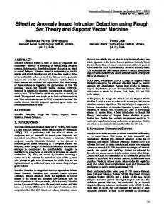
In Step 1 in the algorithm (Fig. 1): • Generate number of trees = M (the population size) using C5. By running C5 M times, and in each run of C5, change the probability of pruning for tree to get different tees. At the end of running C5 method, we store all trees as initial population. •

Divide generates trees over islands and start each island operation.

•

Use heuristic rule to make PGP converge faster [12]. This rule operator operates on the whole population.

Step 1: Master thread start the operation

o

Let R be the attribute set represented by current chromosome. If R is not a hitting set (It is judged in the fitness function computation), Then find an attribute a in C−R which has the maximal value SGF(a, R, D)=p(a).

•

o

If there are several aj, (j=1,2,…,m;) with the same maximal value, stochastically choose one attribute from them.

o

Set the bit corresponding with aj as “1”.

Then according to the fitness for each chromosome; we use stochastic sampling method to select;

In Step 2 in the algorithm (Fig. 2): • Convert the tree into a set of rules (each rule is associated with a complete path in the tree) [4].

Fig 1: Master thread operations

•

Remove the duplicated rules from the set of rules.

•

Compute the fitness value for each set of rules.


30 •

Choose best offspring using following three steps:-

8. Experiment Setup And Results

o

minsingle(Offspring) be the worst individual in the new population, minfit(Offspring) be the corresponding fitness;

o

Let maxsingle(Parent) be the best individual in the old population, maxfit(Parent) be the corresponding fitness.

o

If minfit(Offspring) < maxfit(Parent), we replace minsingel(Offspring) with maxsingle(Parent).

•

Create a new population by applying Crossover, Mutation and Inversion described before.

•

The best-so-far individual is designated as the result of run (i.e. the set of rules).

6.7 Testing Decision System In this step model measure the performance of generated rules on testing data. So this step has following steps:1.

Discretization method is first used to discretizing the new object dataset.

2.

Generated rules are used to match testing objects to compute the strength of the selected rule sets for any decision class.

3.

The new object will be assigned to the decision class with maximal strength of the selected rule set.

7. Parameters Settings The various parameter settings for RSC-PGP are depicted in (Table 2). We made use of +, - , *, /, sin, cos, sqrt, ln, lg, log2, min, max, and abs as function’s set. Table 2: Parameters used by RSC-PGP Parameter

Value Normal

Probe

DoS

U2R

R2L

Population size

100

200

250

100

100

Number of generations

30

200

800

20

800

Chromosome length

30

40

40

30

40

Crossover frequency (%)

90

90

80

90

90

No. of mutations per chromosome

3

4

5

3

4

Branch creation and deletion (%)

5

5

5

5

5

In order to compare RSC-PGA algorithm with other techniques we constructed our intrusion detection system (RSC-PGP) and tested its performance on the KDD-99 intrusion detection contest dataset. As described previously, we are using dataset subset that was preprocessed by the Columbia University and distributed as part of the UCI KDD Archive[21][15]. For each TCP/IP connection, 41 various quantitative and qualitative features were extracted plus 1 class label .The labeling of data features as shown in (Table1) is adopted from Chebrolu [6][15]. The dataset can be classified into five main categories which are Normal, Denial of Service (DoS), Remote to Local (R2L), User to Root (U2R) and Probing. The original data contained 744 MB data with 4,940,000 records. In the International Knowledge Discovery and Data Mining Tools Competition, only “10% KDD-99” dataset is employed for the purpose of training. So, all other experiments performed their analysis on the “10% KDD-99” dataset. In our experiments, we will use this “10% KDD-99” to compare it with other approaches used these data. First of all, in Zainal and Zhang [12] RSC reducts obtained using standard Genetic Algorithms were 26 and they were : C, D, E, F, G, J, M, N, P, W, X, Y, AA, AB, AC, AD, AE, AF, AG, AH, AI, AJ, AK, AL, AM and AN. They had ranked the six most significant features using Rough Set Concept as: C, D, E, X, AF and AO. In addition, there are three different techniques namely Support Vector Decision Function (SVDF), Linear Genetic Programming (LGP) and Multivariate Adaptive Regression Splines (MARS) used by Sung and Mukkamala [7] and one robust model namely Rough Set Classification Parallel Genetic Algorithm (RSCPGA) used by Wa'el, Agiza, and Radwan [22] were used to filter out redundant, superfluous information exist in these features, and hence significantly reduce a number of computer resources, both memory and CPU time, required to detect an attack. SVDF’s proposed features were; B, D, E, W, X and AG. Meanwhile LGP yielded features C, E, L, AA, AE and AI. MARS suggested features E, X, AA, AG, AH and AI. RSC-PGA model has 22 reduct features, and has ranked five most significant features as C, D, E, X, and AO as the core of these reduct features. Our RSC-PGP model has 20 reduct features, and has ranked four most significant features as C, D, E, X as the core of these reduct features. This result is compatible with other approaches results and at the same time contains the "E" reduct feature which has been chosen by other approaches as the most important reduct feature. To compare classification accuracy of our RSC-PGP model with other robust models, we analyzes the True Positive Rate (TPR) and False Positive Rates (FPR) for our model

IJCSNS International Journal of Computer Science and Network Security, VOL.9 No.10, October 2009 with Multi Expression Programming (MEP) and Gene Expression Programming (GEP) models proposed by Abraham, Grosan, and Carlos [1] in order to determine the efficiency of our developed ID model. The TPR value is given by:

DOS

var38 − (Ln(var41 * var6) + sin(Lg(var30))) − (Lg(var30) − (var41 * var6))) > (0.3415 + var24 + var41 * var6)?(var38 − (Ln(var41 * var26) + sin(Lg(var30))) − (Lg(var30) − (var41 * var6))) : (0.3415 + var24 + var41 * var6) + var8

U2R

sin(var14) − var33

R2L

fabs((fabs(var8 > (var1 + (var6 > (Ln(var6))?var6 : (Ln(var6))) * var3)?var10 : (var1 + (var26 > (Ln(var6))?var6 : (Ln(var6))) *var3))) * (var12 + var26)) + var11

The FPR is given by:

As evident from (Table 3), when compared to RSC-PGP obtained the best values for TPR and FPR for Normal, DoS and U2R, and good performance for the other classes. According to column "G" in (Table 3) which shows the required number of generations generated to achieve these result we can see that RSC-PGP also required smallest number of generations for the Probe, DoS, U2R, and R2L types respectively.

31

To make an adequate comparison between the serial GP algorithm and our parallel algorithm to show RSC-PGP speedup, we will run our RSC-PGP model over single thread which will mimic sequential GP algorithm. The parallel speedup is defined as the ratio of the serial execution time to the parallel execution time.

Table 3: Comparison of false alarm rates Attack Type

MEP TPR

GEP

FPR

G

TPR

RSC-PGP

FPR

G

TPR

FPR

G

Normal

0.996

0.999

30

0.996

0.999

35

0.998

0.996

34

Probe

0.947

0.982

60

0.999

0.9748

80

0.997

0.9645

55

Dos

0.987

0.999

200

0.918

0.943

240

0.989

0.990

170

U2R

0.400

0.999

20

0.437

0.995

25

0.443

0.992

18

R2L

0.973

1

90

0.989

0.984

80

0.988

0.989

64

In (Table 4) the variable combinations evolved by RSCPGP is presented. In (Table 4), var represents Variable number (Column 1 in Table 1). It is to be noted that only these few variables are required to detect a particular type of attack. This leads to a very light intrusion detection system when compared to a fuzzy expert system (which requires so many rules) or an artificial neural network with so many hidden neurons [1]. Table 4: Functions evolved by RSC-PGP Attack type Normal

Probe

Evolved Function

var12 * log2(var10 + var3) (fabs(var30 + var35))