Invariant Object Material Identification via Discriminant Learning on

Invariant Object Material Identification via Discriminant Learning on Absorption Features ZhouYu Fu Antonio Robles-Kelly Robby T. Tan Terry Caelli NICTA∗, RSISE Bldg. 115, Australian National University, Canberra, ACT 0200, Australia

Abstract

ysis (LDA)[2], Projection Pursuit [3] and their kernel versions [4] treat raw pixel spectra as input vectors in a higherdimensional space, where the dimensionality is given by the number of bands. The idea is to recover statistically optimal solutions to the classification problem by reducing the dimensionality via a projection of the feature space, often with reduced dimensionality.

In this paper, we propose a novel approach to object material identification in spectral imaging by combining the use of absorption features and statistical machine learning techniques. We depart from the significance of spectral absorption features for material identification and link the use of spectral absorption features with statistical learning. We do this by casting the identification problem into a classification setting which can be tackled using support vector machines. Hence, we commence by proposing a novel method for the robust detection of absorption bands in the spectra. With these bands at hand, we show how those absorptions which are most relevant to the classification task in hand may be selected via discriminant learning. We then train a support vector machine for purposes of classification making use of an absorption feature representation scheme which is robust to varying photometric conditions. We perform experiments on real world data and compare the results yield by our approach with those recovered using an alternative. We also illustrate the invariance of the absorption features recovered by our method to different photometric effects.

From an alternative viewpoint, Clark et al. [6] showed that an unknown spectrum can be identified efficiently by simply matching its dominant absorption feature with a library of spectra and finding the best fit. This is quite interesting, since reflections and absorptions are two complimentary concepts of light behavior. When light reaches the surface of a material, some of it is reflected back, and some is absorbed. While reflections are directly measurable by image sensors, absorptions are less straightforward to recover. Nevertheless, they are inherently related to the material chemistry and, therefore, the presence of an absorption at certain spectral range is often a ”signature” for chemicals and their concentrations. Thus, in contrast with statistical approaches elsewhere in the literature, the use of absorption features for material identification has a clear physical meaning. Here, we investigate the use of statistical learning approaches for purposes of material identification based upon absorption features. The main advantage of this treatment is that, by using absorptions for purposes of identification and recognition, we can perform a localised analysis of the spectra. Hence, the classification task depends solely on the absorption bands. As a result of this treatment, the recognition becomes less sensitive to spectral noise and variations outside the bands under study. Absorptions are also more robust to varying photometric conditions, and, hence, can be used in changing illumination conditions. Furthermore, the use of absorption features opens up the possibility of training statistical classifiers on a small sample set with a marginal detriment on its generalisation properties. The reason is that absorptions are intrinsic to the object material and, also, classification based on absorption is done at a much lower dimension. This contrasts with algorithms elsewhere in the literature, where statistical classification

1. . Introduction With the advent and development of new sensor technology, it is now possible to capture image data in tens or hundreds of bands covering a broad spectral range. Compared to traditional monochrome and trichromatic cameras, hyperspectral image sensors provide richer information on the spectral response of materials over a number of wavelengths. This has posed great opportunities and challenges on material identification. Due to the high dimensional nature of the spectral data, many classical algorithms in pattern recognition and machine learning have been naturally borrowed and adapted so as to perform feature extraction and classification [1]. Techniques such as Principle Component Analysis (PCA), Linear Discriminant Anal∗ National ICT Australia is funded by the Australian Governments Backing Australia’s Ability initiative, in part through the Australian Research Council.

1

methods on the raw spectral data requires a reasonably large training sample set. The outline of this paper is as follows. We commence, in Section 2 by providing some of the background for the material presented throughout the paper. In Section 3, we describe the critical component of the work reported in this paper, namely the feature extraction and classification process. This section, hence, comprises the main contributions of the paper, which are the presentation of an absorption band detection algorithm based upon unimodality, a method for selecting the most discriminant absorption band and the developments on SVM-based classification making use of an invariant absorption feature representation. Section 4 provides an experimental evaluation of the method. Finally, Section 5 offers conclusions on the work.

2. . Prerequisites and Overview Material identification is, in general, a classification problem. In this paper, we model the classification task as a binary classification one, which can be generalised by combining binary classifiers between any two classes [7]. In Fig. 2, we show a diagrammatic representation of our method for feature extraction and classification. As mentioned earlier, our material identification method is based upon a two stage process. The first of these involves the use of absorption features for purposes of training a Support Vector Machine (SVM) classifier. Consider N labelled spectra samples (xi , yi ), where i = {1, . . . , N } and yi ∈ {−1, 1}. To train the SVM, we commence by recovering the absorption bands for each of the samples. This is, we recover the set of all absorption bands occuring in the training data. We then make use of the label information so as to select the most discriminative absorption band that best separates the training samples. Then we truncate the raw spectra and only deal with those spectrum segments considered to be discriminative within the absorption bands. We do this so as to remove the continuum from the segments and apply a transformation to make the spectrum segments under study invariant to specular reflectance artifacts. This treatment yields a set of feature vectors which can be used to train a SVM. With the SVM classifier at hand, we cast the identification task into a classification setting. To do this, we truncate and apply our continuum removal and invariant transformation methods to the test data. We then use the SVM classifier which has been trained using the scheme described above, to make a decision. It is important to note that, in the testing stage, we do not perform absorption band detection and selection to the testing samples. Only simple spectral ratio recovery and spectra processing are involved in obtaining the absorption feature vector. As a result, the computational cost of the testing phase is low.

Figure 1. General Framework for our absorption-based classification algorithm

3. . Absorption Feature Extraction and Classification 3.1. . Absorption Band Detection Recall that absorptions are local ”dips” at certain wavelength range of the spectra. Mathematically, an absorption can be considered as a local valley which breaks the convexity of the local spectrum in nearby bands. In order to recover the absorption features, existing algorithms make use of a scale-space analysis on the derivative of the spectra with respect to wavelength [5, 9, 10]. Here, one common assumption is that the beginning and the end of an absorption band can be located by making use of the inflexion points, which are the zero-crossings of 2nd order derivatives of the spectra. As a result, these methods are prone to noise and quantization effects.Furthermore, there is a tendency to recover absorption bands that are ”narrower” than the true shape of the absorption ”dip”. This is illustrated in Figures 2(a) and 2(c). In this paper, we propose a simple alternative to tackle these problems. Our method is based on continuum removal and unimodal segmentation. The continuum of a spectrum, by definition, is a convex hull fitted over the top of the spectrum so as to connect local spectrum maxima. It can be seen as an envelope spectrum that isolates the absorption bands in the original reflectance spectra. To illustrate this, in Figures 3(a) and 3(b), we have plotted the continuum as a red, dotted line. Following this rationale, we recover the continuum by applying standard convex hull extraction to the original spectrum. The use of convex hull effectively splits the original spectrum into several spectral segments defined over local maxima. These segments assume a concave shape against the continuum, as can be seen in the top panels of Figures 3(a) and 3(b). With the convex hull at hand, we perform continuum removal. This is a standard technology in remote sensing to isolate the local absorption feature from other effects such as level changes and slopes of background absorption [11]. The removal operation is a simple normalization of the raw

spectrum R(λ) with respect to the continuum curve C(λ) such that the continuum removed spectrum r(λ) is given by r(λ) =

R(λ) C(λ)

Absorption Detection by Fingerprint Absorption detection by Unimodal Segmentation

(1)

where λ is, as usual, the wavelength variable. Examples of continuum removed spectra are shown in the bottom plot of Figures 3(a) and 3(b). The spectra shown here have been inverted and normalised in order to turn absorptions into peaks. As we can see, the spectral segments in Figure 3(a) are unimodal, i.e. they only describe a single peak between zero crossings. In contrast, the segment in Figure 3(b) is multimodal with two peaks between zero crossings, which represent two absorption bands. To take our analysis further and recover the absorption features, we make use of a segmentation algorithm based on unimodal regression. The idea is to further segment any absorption into a number of segments, each of which satisfies unimodal constraints. This can be achieved by a two step process. The first step is to split the spectrum into local minima. The second step consists in merging these minima as far as unimodal constraints are satisfied. Here, we enforce unimodal constraints by requiring the error of unimodal fit to be under the threshold value ². In practice, unimodal regression can be implemented in polynomial time through monotonic regression and dynamic programming [12]. Examples of absorption band detection using our method are shown in the right-hand column of Figure 2. In contrast with the standard 2nd order fingerprint method, our method can recover all the absorption bands. Furthermore, the recovered bands are in better accordance with the actual absorptions in the spectra than those yielded by the fingerprint method. In summary, the step sequence for our absorption band detection algorithm is as follows, 1. Recover the convex hull over the spectrum and extract continuum 2. Apply continuum removal and invert the spectrum. 3. For each spectrum segment between two zero crossing points, perform unimodal regression. The stopping criterion for the fitting procedure is given by the threshold ². If the segment is not unimodal, i.e. the fitting error is above the threshold ², perform unimodal segmentation by splitting the segment at the local minima. 4. Merge any two adjacent segments if the unimodal constraint holds for their union. This is done, again, based upon the threshold ². 5. Interleave steps 3 and 4 until no further splitting and merging operations can be performed.

10

20

30

40

50

60

70

80

90

10

20

30

40

band

20

30

40

60

70

80

90

(b) Absorption Detection by Unimodal Segmentation

Absorption Detection by Fingerprint

10

50

band

(a)

50

60

70

80

90

10

20

30

band

40

50

60

70

80

90

band

(c)

(d)

Figure 2. Absorption detection results. Left-hand column: results yield by the Fingerprint method [9]; Right-hand column: results obtained using our unimodal segmentation method.

1

1

0.8

0.8

0.6

0.6

0.4

0.4

0.2

0.2

1/0

1/0

0.8

0.8

Unimodal

0.6

0.4

0.2

0.6

0 0

10

20

30

40

(a)

50

Multimodal

0.6

0.4

60

70

80

90

0 0

10

20

30

40

50

60

70

80

90

(b)

Figure 3. Continuum removal results. Left-hand panel: Continuum removal for a unimodal distribution; Right-hand panel: Continuum removal for a multimodal distribution.

3.2. . Discriminant Absorption Band Selection It should be noted that, despite the accuracy of our method in detecting the absorption bands, not all detected absorptions are significant for purposes of classification. For example, some absorption bands are due to the presence of water and, hence, arise in a wide variety of materials. Furthermore, the spectra of the light source may, potentially, skew the observed absorptions. These ”spurious” absorptions must be eliminated before further processing can be undertaken. In general, there could be a number of absorptions which are not discriminative for classification purposes. Thus, the problem is that of recovering the optimal absorption band (λ1 , λ2 ) in which the spectral segments for positive and negative labelled classes are well separated. This is the so

called discriminative absorption band. To select it, we propose a supervised algorithm based on Linear Discriminant Analysis (LDA) [2] and Kullback-Leibler divergence. The step-sequence of the algorithm is presented in Figure 4.

Given the set of training hyperspectral samples (x1 , y1 ), . . . , (xN , yN ), where yi ∈ {−1, 1} is, as before, the label for the ith sample xi , we compute the set of m extreme spectra values (λ11 , λ12 ), . . . , (λm 1 , λ2 ) for the m absorption bands recovered by our algorithm, as described in the previous section. For each tuple (λi1 , λi2 ), we do the following •

Extract the spectra segments between bands λi1

and λi2 ,

i.e. the recovered absorption segments. • Apply continuum removal to the extracted absorption segments. The continuum for the j th sample is the straight line connecting the values of the spectral sample at the wavelength λi1 and λi2 . • Apply LDA to the continuum removed segments based on label information yj . This is, effectively, a projection of the absorption data onto a one dimensional space. • Choose the tuple (λi1 , λi2 ) that maximises the KL divergence between the two training classes. To this end, we maximise the divergence given by KL = log (

2 σ− σ2 (µ− − µ+ )2 )+ + + 2 2 2 σ+ σ− σ−

(2)

where µ+ , σ+ , µ− , σ− are the mean and standard deviation for the classes with labels 1 and −1, respectively.

the number of bands may be different for two candidate absorptions, the computed KL divergence may be biased towards those absorptions with a greater number of bands. This is regardless of the separability of the two classes as a result of the distributions in higher dimensional spaces being more scattered than those defined in lower dimensions. To balance this effect, we project all the segments to the same dimensional space by making use of LDA as a preprocessing step for the algorithm above. We then compute the KL divergence for the distributions and select the most discriminative absorption band.

3.3. . Invariant Representation In this section, we elaborate on the representation of the absorption features and the invariance of these features to various photometric conditions. In previous studies [6, 10], absorption features are usually represented in parametric form by a 4-element vector, i.e. the extreme spectral bands, the area and the depth of the absorption under study. However, this representation is an empirical one, which lacks theoretical justification. Moreover, it inevitably loses discriminant information due to the lower order statistics which it comprises. In this paper, we adopt a non-parametric representation of the absorption features. We simply use the spectral band-values of the continuum removed spectrum segment within the chosen absorption band given by the tuple (λ1 , λ2 ). As mentioned earlier, we treat these spectral values as feature vectors in a high dimensional space and look at the invariance problem from this perspective. First, note that the extracted absorption feature in the above form is automatically invariant to shading. To see this, consider the diffuse reflectance model for the hyperspectral image under study. For the pixel location u and wavelength λi , the radiance value at wavelength is given by I(λi , u) = g(x)E(λi )S(λi , u)

Figure 4. Discriminant Absorption Band Selection Algorithm

The idea underpinning the algorithm above is that the optimal absorption band should best discriminate between positive and negative spectral classes by maximizing the KL divergence between distributions of corresponding continuum removed spectral segments. It is worth noting that, in the algorithm above, Equation 2 is, in fact, the closed form solution for the KL divergence between two Gaussians. This, in turn, implies that we have assumed the positive and negative sample-set distributions to be Normal in nature. This is a reasonable assumption due to the unimodality of the absorptions. For every candidate absorption band (λi1 , λi2 ), each spectral segment can be seen as a feature vector in N dimensional space, where the dimensionality N is given by the number of bands in the absorption spectral segment. As

(3)

where E(λi ) is the light source spectral component as a function of the wavelength, S(λi , u) is the surface albedo and u is the shading factor at the pixel location u, which depends solely on the geometry of the object. In imaging spectroscopy, we usually deal with reflectance data so as to remove the effects of the light source continuum. This can be achieved, simply, by normalizing I(λi ) with respect to E(λi ). Note that, due to the shading factor, we still cannot recover the true albedo. Nonethelss, we should also notice that, at the normalisation step of the continuum removal process of the previous sections, we are, i ,u) effectively, normalising the ratio R(λi ) = I(λ E(λi ) by the term g(u). As a result, the absorption representation based on the continuum removed spectrum segment is shading invariant. However, the above continuum removed spectrum representation is not invariant to specular effects. This is

due to the fact that specular reflections follow a different model. The Dichromatic model [13] has long been used in physics-based vision for modeling specular reflections for non-lambertian surfaces. The model can be expressed as follows I(λi , u) = g(u)E(λi )S(λi , u) + k(u)E(λi )

(4)

where I(λi , u),g(u),E(λi ) and S(λi , u) are the same as in Equation 3. Compared to the diffuse model, an additional right-hand term has been added to account for the specular reflection. Here, k(u) is the specular factor which depends on the specular geometry at location u. Note that the specular component is a simple scaling of the illumination spectrum independent of the surface albedo. Normalising Equation 4 by the light source spectrum E(λi ), we have R(λi , u) = g(u)S(λi , u) + k(u)

(5)

Now, we see that the second term in the equation above has been reduced to only variable, which depends on the specular geometry term. By taking the difference of reflectance data between two arbitrary bands λi and λj , we can, therefore, eliminate the specular component, i.e. ¡ ¢ R(λi , u) − R(λj , u) = g(u) S(λi , u) − S(λj , u) (6) Now the difference in Equation 6 only depends on the factor g(u), which can be further removed by continuum removal. To summarize, our invariant transformation is outlined as follows. Given the reflectance spectra R(λ, u), the absorption band interval (λ1 , λ2 ) and a band λj ∈ (λ1 , λ2 ), do the following • Take the spectral difference R(λi , u) − R(λj , u), for any λi such that λ1 ≤ λi ≤ λ2 and λi 6= λj • Recover the continuum of the spectral difference by interpolating a line between R(λ1 , u) − R(λj , u) and R(λ2 , u) − R(λj , u). • Apply continuum removal to the spectrum difference.

Notice that all training spectra must be subtracted from the same band λj within the absorption interval. Here, we have chosen the band with minimum mean spectral value, which corresponds to the “valley” of the absorption band. We have done this so as to recover difference spectral values which are positive. Although the above invariant representation holds for normalised reflectance data only, in practice, we can apply it directly to raw spectra if the illumination spectrum is smooth across absorption bands. Despite this will certainly

lead to bias with respect to the true invariant representation, this effect can be compensated by utilising a maximum margin classifier for the discriminant band selection. This assures maximum separability between the two sample classes. Another important invariance we have so far overlooked is the invariance to light source spectra, which is almost impossible to achieve without knowing the spectrum of the illuminant. However, in our experiments, light source variations do not seriously affect the performance. This may be due to the fact that, if the light source has a smooth spectrum in the discriminant absorption band, the unimodal approach presented earlier and the continuum removal step will make illuminant variations appear as Normally distributed errors, which are accounted for by the maximum margin classifier used in our experiments.

3.4. . Feature Classification As mentioned earlier, in this paper, we cast the problem of recognition into a classification setting. Here, we have used, to this end, a Support Vector Machine (SVM) [8]. Amongst all the alternatives in the literature, we have chosen the maximum margin classifier[14], which has been widely used in the pattern recognition, machine learning and computer vision communities. Given the labelled data (xi , yi ), where i = 1, . . . , N and yi ∈ {−1, 1}, the SVM recovers an optimal separating hyperplane which maximises the margin of the classifier. Let wT xi + b = 0 denote this hyperplane, where w is a vector of weights, b is a constant and xi is, as in Section 3, the ith hyperspectral sample. The vector w and the constant b can be found by solving the following constrained optimisation problem, min w,b

X kwk2 +C ²i 2 i

(7)

s.t. yi (wT xi + b) >= 1 − ²i ; i = {1, . . . , N } where ²i >= 0 is the ith slack variable and C is the regularization parameter controlling the trade-off between model complexity and training error. Equation 7 can be transformed into its dual form, whose solution is given by P w = i αi yi xi and b = 1 − ²i − wT xs , where αi >= 0. This holds iff xs is an arbitrary support vector for which the constraint in Equation 7 becomes an equality. In the linearly inseparable case, we can apply a nonlinear, kernel-based transformation to the input vectors by projecting them to a high dimensional space. In this way, the optimal separating plane can be found. Though the exact mapping of the input vector to the nonlinear feature space usually can not be obtained, the inner product between two projected feature vectors can be computed efficiently via substituting xi with a kernel function φ(xi ). Thus, in the

nonlinear case, the optimal hyperplane becomes X wT φ(xi ) + b = αi yi K(xj , xi ) + b = 0

Training Spectra Positive samples (healthy region) Negative samples (scabbed region)

(8)

i

where K(xj , xi ) = φ(xj )T φ(xi ) is the inner product between feature vectors. Written in this manner, w and b can be obtained by solving the same quadratic programming problem as in Equation 7. There are different options for the kernels used in nonlinear SVMs. In this paper, we choose the Radial Basis Function kernel given by K(xj , xi ) = exp (−βkxj − xi k2 ) where β is a scale parameter.

500

550

600

650

700

band(nm)

(a)

(b)

(c)

(d)

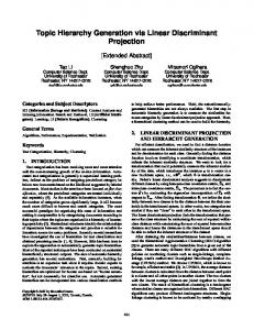
4. . Experimental Results Having presented the theoretical foundation for our method, in this section we perform experiments so as to demonstrate the performance of our algorithm on imagery of apples infected with the fungus Venturia inaequalis and wheat infected with rust (Puccinia striformis). We have collected our imagery using a hyperspectral camera system from Opto-Knowledge Systems Inc (OKSI) [15], which is comprised by a broad band monochrome camera and a Varispec liquid crystal tunable filter (LCTF) manufactured by Cambridge Research Instruments (CRI). The spectral resolution of the imagery is of 10nm between the 400nm to 720nm wavelengths, i.e. 33 bands in the visible spectrum. The image spatial resolution is 696 by 520 pixels. First, we turn our attention to the apple data. In the first experiment, a hyperspectral image of two infected Granny Smith apples was taken against black background under an artificial sunlight illuminant with Correlated Colour Temperature (CCT) of 5500K. Each pixel in the image was then normalised by the sunlight illumination spectrum to get the reflectance data. The pseudo-colour image is shown in left-hand panel of the top row of Figure 5(a). For training purposes, two small areas in the image were selected in one from the image depicting healthy tissue and the other from the one comprising infected tissue. These areas are those within the black and red rectangles drawn on the image. Pixel spectra plots of positive (healthy) and negative (infected) labelled samples from the selected regions are shown in Figure 5(b). After running our absorption band detection and selection algorithms, the optimal absorption band leading to maximum discriminability between the two classes was found to be between 560nm and 700nm, as indicated by black arrows in Figure 5(b). We have then trained the SVM classifier on the invariant absorption features to get our classification model. For this purpose, we used the LIBSVM package [16]. The SVM parameters were chosen by 5-fold cross validation. With the trained SVM classifier at hand, we have run tests on all foreground pixels in Fig 5(a). For visualisation purposes, we have mapped the test result back to the image

Figure 5. (a) Pseudo-colour apple image; (b) Spectra of the training pixels. Red plots correspond to infected tissue and green traces to healthy tissue; (c) Surface map inferred by our algorithm. (d) Surface map inferred by the direct application of the SVM classifier to the raw spectral data.

so as to indicate the probability of the apple tissue being healthy at a given pixel location. The inferred surface map is shown in Figure 5(c). In the figure, pixel brightness indicates the status of the tissue at the corresponding pixel location. The brighter the pixel, the more probable is that the apple tissue is healthy at the location under study. For purposes of comparison, we have also trained an SVM classifier directly on the reflectance spectra. At the training stage, each band was properly scaled before a spectrum vector was input to the SVM. As in our method, the parameters of SVM were also chosen from 5-fold cross validation. The surface map inferred by directly applying the SVM classifier to the pixel spectra is shown in Figure 5(d). From the figures, it becomes evident that the inferred surface map is prone to shading effects, where pixels near the boundary of the apple are significantly darker than pixels in the center. This incorrectly indicate that regions near the boundary are not as healthy as regions in the center. In contrast with this, the surface map inferred by our algorithm, based on invariant absorption features, is shading invariant. Moreover, some specular pixels were incorrectly labeled as “unhealthy” by direct SVM application, while our algorithm correctly identifies these pixels as healthy ones. To further illustrate the invariance of our absorption representation to specularities, we have selected pixels from different regions on the apple which show a number of photometric conditions. These are those pixels in regions labeled A, B, C in Figure 6(a). There is almost no shading for region A, while region B is highly shaded and region C is highly specular. Their corresponding spectra are plotted in Figure 6(b). The absorption features extracted making use of our invariant representation have been plotted in Figure

Spectra of selected regions

Absorption feature of front region Absorption feature of shaded region

Spectra of specular region

Absorption feature of specular region

500

550

band(nm)

(a)

Absorption features of selected regions

Spectra of front region Spectra of shaded region

(b)

600

650

700

2

4

6

8

10

12

14

band

(c)

Figure 6. (a) Apple with different regions selected; (b) Spectra for those pixels in the selected regions. Each colour corresponds to different photometric conditions; (c) Invariant absorption features delivered by our algorithm.

6(c). It can be clearly seen that the absorption features recovered in this manner show a good degree of invariance to shading and specular effects. To take our analysis further, we have have been taken apple images under different illuminations than the one from which the model training samples were drawn. We took two more hyperspectral images of exactly the same apples. The first of these, shown in Figure 7(a), making use of an artificial sunlight. The second, shown in Figure 7(b), taken under yellow halogen light. With the images at hand, we have attempted to classify, making use of the SVMs trained in the previous experiment, the apple tissue captured in the new imagery. The surface maps inferred by our algorithm are shown in the middle row of Figure 7. Again, we have compared our experiments with those results yield using the raw pixel spectra as input features. The results of directly running the SVM on the raw pixel spectra are shown in bottom row of Figure 7. In contrast with the SVM classifier based on the raw spectra, our algorithm still yields good results for testing data obtained from different illumination conditions. We now turn our attention to the wheat infected with stem rust. This is a more challenging classification example for which we provide a quantitative analysis. Two hyperspectral images were taken for two specimens of wheat, one healthy and one infected, illuminated from two different light source directions. The pseudo-colour images are shown in the top row of Figure 8. In both panels, the healthy wheat was placed in the left-hand side and the infected wheat on the right-hand side. The two images differ only in terms of light source direction. For the image in Figure 8(a), the illuminant was placed approximately 45o left of the camera axis. In Fig. 8(a), the light source direction is approximately 45o right of the camera direction. The healthy and infected plants look very similar and is hard to distinguish them by colour. We randomly picked 100 pixels from both, the healthy and the deceased wheat from the image in Figure 8(a). The plots for the spectra of these pixels are shown in Figure 8(c). From the plots, its clear that, despite the intensity, the spectral traces for both specimens have similar shapes. We apply our discriminant band selection algorithm to select the most discriminative absorption band, which is between 550nm and 720nm, as indicated by

(a)

(b)

(c)

(d)

(e)

(f)

Figure 7. Top row: apples under artificial sunlight and halogen light; Middle row: surface maps inferred by our algorithm. Bottom row: surface maps inferred by SVM.

the black arrows in Figure 8(c). The plots for the invariant absorption features recovered by our algorithm are shown in Figure 8(d), where green curves denote features of healthy wheat and red traces correspond to infected wheat. Since the healthy and the infected wheat were placed apart, we can easily separate and label them from the images to obtain ground truth data. To provide a quantitative analysis, we have randomly selected pixels from the healthy and the infected wheat samples in Figure 8(a). We have then trained the classifiers using both, the absorption features delivered by our algorithm and the raw spectra and tested the SVMs on the images under study. For our analysis, different number of training pixels were chosen from each class, ranging from 10 to 1000. In Figure 9, we show some surface maps inferred by our algorithm and the alternative using a training sample size of 100. The surface maps recovered from Figure 8(a), shown in Figures 9(a) and 9(b), are quite similar for the two algorithms. Nonetheless, the surface map inferred by our algorithm for Figure 8(a), shown in Figure 9(d), is better than that delivered by the alternative (Figure 9(d)). In Table 1, we show the classification error rates and variances for our algorithm (ABS+SVM) and the alternative (SVM). For purposes of verification, we have repeated each pair of training-test operations 5 times, every one of these with a different set of randomly selected training pixels. Again, the SVM parameters were chosen from 5-fold

(a)

(b)

(a)

(b)

(c)

(d)

Spectra of healthy and rusted wheat Absorption features of healthy and rusted wheat

Spectra of healthy wheat Healthy wheat

Spectra of rusted wheat

Rusted wheat

500

550

600

650

2

700

4

6

8 band

band

(c)

10

12

14

16

(d)

Figure 8. (a) and (b) Pseudo Images of wheat illuminated from different directions; (c) Wheat spectra; (d) Absorption features recovered by our algorithm. Table 1. Error rates and variances for our method (ABS+SVM) and the alternative (SVM)

Error rate(%) Sample size

Image 1 SVM ABS+SVM

Image 2 SVM ABS+SVM

10

19.35 ± 3.79 16.81 ± 3.66 25.39 ± 10.06 17.41 ± 3.10

50

7.28 ± 1.87

7.12 ± 1.21

10.27 ± 2.56

6.99 ± 1.34

100

4.78 ± 0.34

5.17 ± 0.70

7.68 ± 2.38

5.62 ± 0.45

500

3.50 ± 0.27

3.79 ± 0.27

9.18 ± 4.81

4.96 ± 0.12

1000

3.10 ± 0.14

3.30 ± 0.05

6.82 ± 3.82

4.63 ± 0.36

cross validation and proper scaling was applied to the raw spectra input vectors to ensure optimal tuning of the SVM classifiers. From Table 1, our method is more stable, performancewise, than the direct application of SVMs to the raw spectra. First, while blind SVM training can do quite a good job on the image from where the training samples were selected, it fails to classify as accurately as our absorption-based algorithm the data on the image in Figure 8(b). This problem can be somehow alleviated by using more training samples, but in the case of our method, no matter how many training samples are used, the performance is always better than that of the alternative when the image in Figure 8(b) is used for testing purposes. Second, the variation of the test results for the raw spectral data is larger than that for our algorithm. As training samples are chosen randomly, this indicates that the alternative relies more on the quality of the training samples, i.e. it requires the use of clean data for training, while our algorithm is more robust to noise and, hence is less limited on the choice of the training sampleset. Third, the alternative requires a reasonably large sample set for training. With increasing number of samples in each class, the performance of the algorithm based upon the raw spectra also increased. Although our algorithm also needs

Figure 9. Results yield by the two algorithms. (a),(c) Surface maps inferred by our algorithm; (b),(d) Results yield by the alternative.

a number of training samples, it outperforms the alternative for small training sample sizes.

. Conclusion 5. In this paper, we have presented a novel recognition method which exploits absorption features for invariant material identification under changing photometric conditions. To this end, we have adopted an invariant representation and developed a method in which the optimal absorption band was automatically learned from training data via statistical analysis. We have illustrated the utility of the method for purposes of identification on real world imagery, where our algorithm compares favorably with blind SVM classification on raw spectral data.

6. Acknowledgment The authors are indebted with the Cooperative Research Centre for National Plant Biosecurity (CRC for Plant Biosecurity), Australia, for facilitating them the apple and wheat samples used in the experimental section of this paper.

References [1] D. Landgrebe, “Hyperspectral Image Data Analysis,” IEEE Signal Processing Mag.,19:17-28, 2002 1 [2] K. Fukunage, Introduction to Statistical Pattern Recognition, 2nd Ed., Academic Press, NY, 1990 1, 4 [3] L. Jimenez, D. Landgrebe, “Hyperspectral Data Analysis and Feature Reduction via Projection Pursuit,” IEEE Trans. on Geoscience and Remote Sensing, 37(6):2653-2667, 1999 1 [4] M. Dundar, David Landgrebe, “Toward an Optimal Supervised Classifier for the Analysis of Hyperspectral Data,” IEEE Trans. on Geoscience and Remote Sensing, 42(1), 271-277, 2004 1 [5] T. M. Lillesand, R. W. Kiefer, “Remote Sensing and Image Interpretation,” John Wiley and Sons, 1999 2 [6] R. Clark, G. Swayze, K. Livo, R. Kokaly, S. Sutley, J. Dalton, R. McDougal, C. Gent, “Imaging Spectroscopy: Earth and Planetary Remote Sensing with the USGS Tetracorder and Expert System,” Journal of Geophysical Research, 108(5):1-44, 2003 1, 4

[7] T. Hastie, R. Tibshirani “Classification by Pairwise Coupling,” Proc. of Neural Information Processing Systems, 1997 2 [8] N. Cristianini and J. Shawe-Taylor, “An Introduction to Support Vector Machines,” Cambridge University Press, 2000. 5 [9] M. Piech, K. Piech, “Symbolic Representation of Hyperspectral Data,” Applied Optics, 26:4018-4026, 1987 2, 3 [10] P. Hsu, “Spectral Feature Extraction of Hyperspectral Images using Wavelet Transform,” Ph.D. thesis, Dept. of Survey Engineering, National Cheng Kung Univ., Taiwan, China, July 2003 2, 4 [11] R. Clark, T. Roush, “Reflectance Spectroscopy: Quantitative Analysis Techniques for Remote Sensing Applications,” Journal of Geophysical Research, 89:6329-6340, 1984 2 [12] Q. F. Stout, “Optimal algorithms for unimodal regression,” Computing Science and Statistics, 32, 2002 3 [13] S. Shafer, “Using Color to Separate Reflection Components,” Color Research and Applications, 10:210-218, 1985 5 [14] L. Xu, J. Neufeld, B. Larson, and D. Schuurmans. “Maximum margin clustering,” In Advances in Neural Information Processing Systems 17, pages 1537–1544. MIT Press, 2004. 5 [15] N. Gat “Imaging Spectroscopy Using Tunable Filters: A Review,” SPIE Conf. Algorithms for Multispectral and Hyperspectral Imagery VI, 4056:50-64, 2000 6 [16] “LIBSVM: a library for support vector machines,” http://www.csie.ntu.edu.tw/˜cjlin/libsvm, 2001 6