Inverse Engineering a simple Real Time program - Martin Ward

Inverse Engineering a simple Real Time program E. J. Younger

M. P. Ward

Centre for Software Maintenance Ltd Unit 1P Mountjoy Research Centre Durham, DH1 3SW

Computer Science Department Science Labs South Rd Durham DH1 3LE

January 17, 2003 Abstract Reverse engineering of interrupt-driven real-time programs with timing constraints is a particularly challenging research area, because the functional behaviour of a program, and the non-functional timing requirements, are implicit and can be very difficult to discover. However, in this paper we present a significant advance in this area, which is achieved by modelling real-time programs with interrupts in the wide spectrum language WSL. A small example program is modelled in this way, and formal program transformations are used to derive various timing constraints and to “inverse engineer” a formal specification of the program. (We use the term “inverse engineering” to mean “reverse engineering achieved by formal program transformations).

1

Introduction

This paper describes the process by which a simple interrupt-driven real time program has been modelled in WSL and subsequently inverse engineered to derive a specification for the program. The example is based on a previous case study, which we have simplified somewhat in order to concentrate on the handling of interrupts and timing information without the additional complications inherent in that system. The example is a simple program which runs in an infinite loop, reading characters from a circular buffer and printing these on the standard output. Characters are placed into the buffer by an interrupt routine, which may be triggered by external hardware, or another concurrent process. When the buffer is empty, the program simply waits for more characters. Our objectives in reverse engineering this program were as follows: 1. To derive a specification for the system, and thus 2. To show that there was no interference between the main program and the interrupt code, i.e. to demonstrate that the points in its execution at which the main program is interrupted are not significant—all such interrupts are equivalent. Alternatively if there is interference then we should expect to identify where it occurs 3. To derive the combinations of timing constraints on interrupts, and buffer requirements, which will guarantee that the program functions correctly. The paper is organised as follows. In sections 2 and 3 we give a brief introduction to the WSL language and transformation theory. Then in Section 4 we show how to model a real-time interrupt-driven program in the WSL language. In Section 5 we transform the WSL model into a simpler form, from which the timing constraints are derived in Section 6. Finally, we use this information to derive a specification of the program in Section 7. 1

2

The Language WSL

In this section we give a brief introduction to the language WSL [13,42,44,45,48] the “Wide Spectrum Language”, used in Ward’s program transformation work, which includes low-level programming constructs and high-level abstract specifications within a single language. By working within a single formal language we are able to prove that a program correctly implements a specification, or that a specification correctly captures the behaviour of a program, by means of formal transformations in the language. We don’t have to develop transformations between the “programming” and “specification” languages. An added advantage is that different parts of the program can be expressed at different levels of abstraction, if required. A program transformation is an operation which modifies a program into a different form which has the same external behaviour (it is equivalent under a precisely defined denotational semantics). Since both programs and specifications are part of the same language, transformations can be used to demonstrate that a given program is a correct implementation of a given specification. In [43, 46,47,49] program transformations are used to derive a variety of efficient algorithms from abstract specifications. 2.1

Syntax of Expressions

Expressions include variable names, numbers, strings of the form “text...”, the constants N, R, Q, Z, and the following operators and functions. Note that since WSL is a wide spectrum language it must not be restricted to finite values and computable operations. In the following e 1 , e2 , etc., represent any valid expressions: Numeric operators: e1 + e2 , e1 − e2 , e1 ∗ e2 , e1 /e2 , ee12 and so on, with the usual meanings. Sequences: s = ha1 , a2 , . . . , an i is a sequence, the ith element ai is denoted s[i], s[i . . j] is the subsequence hs[i], s[i + 1], . . . , s[j]i, where s[i . . j] = hi (the empty sequence) if i > j. The length of sequence s is denoted `(s), so s[`(s)] is the last element of s. We use s[i . . ] as an abbreviation for s[i . . `(s)]. reverse(s) = han , an−1 , . . . , a2 , a1 i, head(s) is the same as s[1] and tail(s) is s[2 . . ]. Sequence concatenation: s1 ++ s2 = hs1 [1], . . . , s1 [`(s1 )], s2 [1], . . . , s2 [`(s2 )]i. The append function, append(s1 , s2 , . . . , sn ), is the same as s1 ++ s2 ++ · · · ++ sn . Subsequences: The assignment s[i . . j] := t[k . . l] where j − i = l − k assigns s the value hs[1], . . . , s[i − 1], t[k], . . . , t[l], s[j + 1], . . . , s[`(s)]i. Stacks: Sequences are also used to implement stacks, for this purpose we have the following pop notation: For a sequence s and variable x: x ←− s means x := s[1]; s := s[2 . . ] which pops an element off the stack into variable x. To push the value of the expression e onto push stack s we use: s ←− e which represents: s := hei ++ s. cons(e, s) is the same as hei ++ s. last

Queues: The statement x ←− s removes the last element of s and stores its value in the variable x. It is equivalent to x := s[`(s)]; s := s[1 . . `(s) − 1]. Sets: We have the usual set operations ∪ (union), ∩ (intersection) and \ (set difference), ⊆ (subset), ∈ (element), ℘ (powerset). { x ∈ A | P (x) } is the set of all elements in A which satisfy predicate P . For the sequence s, set(s) is the set of elements of the sequence, i.e. set(s) = { s[i] | 1 6 i 6 `(s) }. The expression #A denotes the size of the set A. 2.2

Syntax of Formulae

In the following Q, Q1 , Q2 etc., represent arbitrary formulae and e1 , e2 , etc., arbitrary expressions: Relations: e1 = e2 , e1 6= e2 , e1 < e2 , e1 6 e2 , e1 > e2 , e1 > e2 , equal(e1 , e2 ), eq(e1 , e2 ), even?(e1 ), odd?(e1 ); Logical operators: ¬Q, Q1 ∨ Q2 , Q1 ∧ Q2 ; 2

Quantifiers: ∀v. Q, ∃v. Q. 2.3

Syntax of Statements

In the following, S1 , S2 etc., are statements, Q, B etc., are formulae, and x is either a finite sequence of variables or a simple variable and t is either a finite sequence of expressions or a single expression. x0 is the sequence hx01 , . . . i if x is the sequence hx1 , . . . i. Sequential composition: S1 ; S2 ; S3 ; . . . ; Sn Deterministic choice: if B then S1 else S2 fi Assertion: {B}. An assertion is a partial skip statement, it aborts if the condition is false but does nothing if the condition is true. Assignment: x := x0 .Q. This assigns new values x0 to x such that the formula Q is true. If there are no values which satisfy Q then the statement does not terminate. For example, the assignment hxi := hx0 i.(x = 2.x0 ) halves x if it is even and aborts if x is odd. If the sequence contains one variable then the sequence brackets may be omitted, for example: x := x0 .(x = 2.x0 ). Simple assignment: x := t. This assigns the values of the expressions t to the variables in x. The single assignment hxi := hti can be abbreviated to x := t. µ operator: x := µx0 .Q. This assigns to x the smallest non-negative integer value x0 such that the formula Q becomes true. It is equivalent to: x := x0 .(Q ∧ x0 ∈ N0 ∧ ∀x00 ∈ N0 . (x00 < x0 ⇒ ¬Q[x00 /x0 ])) where N0 is the set of non-negative integers and Q[x00 /x0 ] is Q with all occurrences of variable x0 replaced by x00 . Nondeterministic choice: The “guarded command” of Dijkstra [17]: if B1 → S1 t u B2 → S 2 ... t u Bn → Sn fi Each of the “guards” B1 , B2 , . . . , Bn is evaluated, one of the true ones is selected and the corresponding statement executed. If no guard is true then the statement aborts. Deterministic iteration: while B do S od The condition B is tested and S is executed repeatedly until B becomes false. Nondeterministic iteration: The “guarded command loop” of Dijkstra [17]: do B1 → S1 t u B2 → S 2 ... t u Bn → Sn od This is equivalent to: while B1 ∨ B2 ∨ · · · ∨ Bn do if B1 → S1 t u B2 → S2 ... t u Bn → Sn fi od Uninitialised local variables: var x : S end Here x is a local variable which only exists within the statement S. It must be initialised in S before it is first accessed. Initialised local variables: var x := t : S end This is an abbreviation for var x : x := t; S end. The local variable is initialised to the value t. We can combine initialised and uninitialised variables in one block, for example: var x := t, y : S end where x is initialised and y is uninitialised. 3

Counted iteration: for i := b to f step s do S od is equivalent to: var i := b : while i 6 f do S; i := i + s od end Unbounded loops and exits: Statements of the form do S od, where S is a statement, are “infinite” or “unbounded” loops which can only be terminated by the execution of a statement of the form exit(n) (where n is an integer, not a variable or expression) which causes the program to exit the n enclosing loops. To simplify the language we disallow exits which leave a block or a loop other than an unbounded loop. This type of structure is described in [27] and more recently in [40]. 2.4

Procedures and Functions with Parameters

We use the following notation for procedures with parameters: begin S1 where proc F (x, y) ≡ S2 . end where S1 is a program containing calls to the procedure F which has parameters x and y. The body S2 of the procedure may contain recursive procedure calls. We use a similar notation (with funct instead of proc) for function calls.

3 3.1

Program Refinement and Transformation Transformation Methods

The Refinement Calculus approach to program derivation [23,31,32] is superficially similar to our program transformation method. It is based on a wide spectrum language, using Morgan’s specification statement [30] and Dijkstra’s guarded commands [17]. However, this language has very limited programming constructs: lacking loops with multiple exits, action systems with a “terminating” action, and side-effects. These extensions are essential if transformations are to be used for reverse engineering. The most serious limitation is that the transformations for introducing and manipulating loops require that any loops introduced must be accompanied by suitable invariant conditions and variant functions. This makes the method unsuitable for a practical reverse-engineering method. A second approach to transformational development, which is generally favoured in the Z community and elsewhere, is to allow the user to select the next refinement step (for example, introducing a loop) at each stage in the process, rather than selecting a transformation to be applied to the current step. Each step will therefore carry with it a set of proof obligations, which are theorems which must be proved for the refinement step to be valid. Systems such as µral [25], RAISE [34] and the B-tool [1] take this approach. These systems thus have a much greater emphasis on proofs, rather than the selection and application of transformation rules. Discharging these proof obligations can often involve a lot of tedious work, and much effort is being exerted to apply automatic theorem provers to aid with the simpler proofs. However, Sennett in [38] indicates that for “real” sized programs it is impractical to discharge much more than a tiny fraction of the proof obligations. He presents a case study of the development of a simple algorithm, for which the implementation of one function gave rise to over one hundred theorems which required proofs. Larger programs will require many more proofs. In practice, since few if any of these proofs will be rigorously carried out, what claims to be a formal method for program development turns out to be a formal method for program specification, together with an informal development method. For this approach to be used as a reverse-engineering method, it would be necessary to discover suitable loop invariants for each of the loops in the given program, and this is very difficult 4

in general, especially for programs which have not been developed according to some structured programming method. The Munich project CIP (Computer-aided Intuition-guided Programming) [6,7,8] uses a widespectrum language based on algebraic specifications and an applicative kernel language. They provide a large library of transformations, and an engine for performing transformations and discharging proof obligations. The kernel is a simple applicative language which uses only function calls and the conditional (if. . . then) statement. This language is provided with a set of “axiomatic transformations” consisting of: α-, β-and η-reduction of the Lambda calculus [15], the definition of the if-statement, and some error axioms. Two programs are considered “equivalent” if one can be reduced to the other by a sequence of axiomatic transformations. The core language is extended until it resembles a functional programming language. Imperative constructs (variables, assignment, procedures, while-loops etc.) are introduced by defining them in terms of this “applicative core” and giving further axioms which enable the new constructs to be reduced to those already defined. Similar methods are used in [12,37,53] and [9]. However this approach does have some problems with the numbers of axioms required, and the difficulty of determining the exact correctness conditions of transformations. These problems are greatly exacerbated when imperative constructs are added to the system. Problems with purely algebraic specification methods have been noted by Majester [29]. She presents an abstract data type with a simple constructive definition, but which requires several infinite sets of axioms to define algebraically. In addition, it is important for any algebraic specification to be consistent, and the usual method of proving consistency is to exhibit a model of the axioms. Since every algebraic specification requires a model, while not every model can be specified algebraically, there seems to be some advantages in rejecting algebraic specifications and working directly with models. 3.2

Transformation Systems

Many workers have recognised that developing a program by successive transformation can be made much easier and less error-prone if an interactive or automatic system is provided which can carry out the transformations, perhaps check that they are used in a valid way, and keep a record of the various versions of the program. Thus, there has been much research into transformational programming and this has resulted in a large number of experimental systems. For a detailed overview of these see the papers by Partsch and Steinbr¨ ugen [36] and Feather [19]. The three main types of transformation system are: 1. A manual system makes the user responsible for every single transformation step. It is the simplest implementation and the system must provide some means for building up compact and powerful transformation rules. 2. A fully automatic system enables the selection and appropriate rules to be completely determined by the system using built-in heuristics, machine evaluation of different possibilities, or other strategic consideration. 3. A semi-automatic system works both autonomously for predefined subtasks and manually for unsolvable problems. For such systems there are two main ways of organising the transformations: The first is as an extensible catalogue of specific transformations, the second is to have a small “generative set” of very simple transformations which are combined in various ways to provide more powerful manipulations. The Cornell Program Synthesiser of [5,41] can be thought of as a totally manual system. It is an interactive system for program writing and editing which acts directly on the structure of the program by inserting and deleting structures in such a way as to ensure that the edited program is always syntactically correct: used as a transformation system, the user would be responsible for

5

the semantic correctness of the manipulations. Arsac [2] describes using a simple manual system to carry out transformations of a program and store the various versions. His system knows some transformations but makes no attempt to check that the correctness conditions of a transformation hold when it is applied. The first work on automatic program transformation was done by Burstall and Darlington in the mid-1970’s [14]. Their first system was based on a schema-driven method for transforming applicative recursive programs into imperative ones: with the ultimate goal of improved efficiency. The system worked largely automatically, according to a set of built-in rules, with only a small amount of user control. The rules were simple transformations, including recursion removal, elimination of redundant computations, unfolding and structure sharing. Their second system, implemented in POP-2 and designed to manipulate applicative programs, is a typical representative of the generative set approach and consists of only six rules: definition, instantiation, unfolding, folding, abstraction, and laws (actually a set of data-structure-specific rules). “Definition” allows the introduction of the new functions (in the form of recursion equations). Balzer built a program transformation system in the early 1980’s [4]. The system used a separate specification language GIST, rather than a single wide-spectrum language. The CIP-S transformational system [8], based on the CIP-L language [6], aims to develop an integrated environment for the transformational development of programs from algebraic specifications. This includes manipulation of concrete programs, derivation of new transformational rules within the system, transformation of algebraic types, and verification of applicability conditions, and the documentation of developments and their manipulation. The DRACO System is a general mechanism for software construction based on the paradigm of “reusable software”. “Reusable” here means that the analysis and design of some library program can be reused, but not its code. DRACO is an interactive system that enables a user to refine a problem, stated in a high level problem domain specific language, into an efficient LISP program. Accordingly, DRACO supplies mechanisms for defining problem domains as special purpose domain languages and for manipulating statements in these languages into an executable form. Another automatic system, the DEDALUS system (DEDuctive ALgorithm Ur-Synthesizer) by Manna and Waldinger is implemented in QLISP. Its goal is to derive LISP programs automatically and deductively from high-level input-output specifications in a LISP-like representation of mathematical logic notation. A goal-directed deductive approach is used whereby the reduction of a goal (to synthesize a program satisfying a given specification) to one or more subgoals, by means of a transformation rules, results in the generation of a program fragment which computes the desired result, once it is completed with program fragments corresponding the subgoal(s). So, for example, reducing a goal to two subgoals by means of a case analysis corresponds to the introduction of a conditional expression. The long-running SETL project at the Courant Institute of New York University [16] has served as the context for a wide variety of transformation research. Their very high level programming language, SETL, has syntax and semantics based on standard mathematical set theory. SETL programs can always be executed; however, na¨ıve execution of programs that make liberal use of the high-level language features may be very inefficient. The SETL compiler has been built to compile SETL programs into efficient interpretable code or machine code. Used in this manner, the SETL compiler would fall into the category of a traditional compiler, albeit a very sophisticated one. Boyle’s TAMPR (Transformation-Assisted Multiple Program Realization) system provides a variety of support for programming in FORTRAN at the Argonne National Laboratory [11]. The modest nature of the tasks attempted enables TAMPR’s transformation process to be entirely automatic. In addition to transformation within the FORTRAN language, TAMPR has also been 6

applied to help in FORTRAN-to-PASCAL translation, and in converting the bulk of the TAMPR system itself from its (almost) pure applicative LISP version into FORTRAN (which runs faster than compiled LISP form on the same machine). This latter application demonstrates the feasibility of the approach on moderately large programs (1300 lines, 42 functions, converted into 3000 lines of FORTRAN). Boyle stresses that approaching these tasks by means of program transformation encourages organising it in a modular fashion, with many consequent benefits. Feather’s ZAP system and language [20] is based on the fold/unfold work of Burstall and Darlington on transforming applicative programs expressed in recursion equations. The ZAP system’s language is a language for expressing transformations and developments. The KIDS system (Kestrel Interactive Development System) [39] is based on axiomatic specifications and purely functional programs. Program synthesis is based on building a “theory morphism” from an algorithm theory (e.g. global search) to a problem theory (e.g. n-queens). The prototype implementation has produced some small runnable programs. The Popart system [52] uses automatic invocation of sets of transformations with declarative user guidance. It uses “Extended BNF” as a specification language and Lisp, Ada and C ++ as target languages. There is a metaprogramming language (Paddle) for ad hoc transformational developments. The PROSPECTRA system [28] attempted to compile algebraic specifications into purely functional programs. 3.3

Automating the Process

There are currently three main ways of automating more of the transformation process (see [22]): Jittering: The method used in the Transformational Implementation (TI) system developed by Balzer [4], and also in Fickas’ GLITTER system [21] is that of jittering. In this system, if a transformation is applied, but fails due to some minor technical detail, the system automatically modifies the program (using transformations) so that the initial transformation can succeed. Means-end analysis: A variant of jittering, called means-end analysis, is used by Mostow [33] to guide rule selection. The user provides the pattern to be matched in order to apply the rule, and the system computes the difference between this and the actual current pattern. The computed difference then indexes further rules which could be used to reduce the difference. Optimal “Next” Transformations: In this approach, the system is tried manually on many different programs and the order of transformations used is recorded; this is a knowledge elicitation process (and will also be used in the next approach to determine what metrics to use). From these results it will be possible to determine which transformations form sequences and to make suggestions as to the next transformation to use based on the previous one. For example, removing a redundant variable may follow merging two assignments. The Metric Approach: The final approach is, perhaps, the most ambitious. This is to determine a metric which quantifies the “ease of understanding”, or “niceness”, of a program and uses “hill-climbing” methods to find a sequence of transformations which manipulate the program into an equivalent form which maximises this metric. Note that total automation is extremely difficult and probably undesirable: the best approach is an interactive system which is highly automated in some areas (eg restructuring). 3.4

Our Approach

In developing a model based theory of semantic equivalence, we use the popular approach of defining a core “kernel” language with denotational semantics, and permitting definitional extensions in terms of the basic constructs. In contrast to other work (for example, [7,10,35]) we do not use a 7

purely applicative kernel; instead, the concept of state is included, using a specification statement which also allows specifications expressed in first order logic as part of the language, thus providing a genuine wide spectrum language. Fundamental to our approach is the use of infinitary first order logic (see [26]) both to express the weakest preconditions of programs [17] and to define assertions and guards in the kernel language. Engeler [18] was the first to use infinitary logic to describe properties of programs; Back [3] used such a logic to express the weakest precondition of a program as a logical formula. His kernel language was limited to simple iterative programs. We use a different kernel language which includes recursion and guards, so that Back’s language is a subset of ours. We show that the introduction of infinitary logic as part of the language (rather than just the metalanguage of weakest preconditions), together with a combination of proof methods using both denotational semantics and weakest preconditions, is a powerful theoretical tool which allows us to prove some general transformations and representation theorems. The WSL language includes both specification constructs, such as the general assignment, and programming constructs. One aim of our program transformation work is to develop programs by refining a specification, expressed in first order logic and set theory, into an efficient algorithm. This is similar to the “refinement calculus” approach of Morgan et al [23,31]; however, our wide spectrum language has been extended to include general action systems and loops with multiple exits. These extensions are essential for our second, and equally important aim, which is to use program transformations for reverse engineering from programs to specifications. In [48] we describe our method for formal reverse engineering using transformations. Refinement is defined in terms of the denotational semantics of the language: the semantics of a program S is a function which maps from an initial state to a final set of states. The set of final states represents all the possible output states of the program for the given input state. Using a set of states enables us to model nondeterministic programs and partially defined (or incomplete) specifications. For programs S1 and S2 we say S1 is refined by S2 (or S2 is a refinement of S1 ), and write S1 ≤ S2 , if S2 is more defined and more deterministic than S1 . If S1 ≤ S2 and S2 ≤ S1 then we say S1 is equivalent to S2 and write S1 ≈ S2 . Equivalence is thus defined in terms of the external “black box” behaviour of the program. A transformation is an operation which maps any program satisfying the applicability conditions of the transformation to an equivalent program. See [42] and [44] for a description of the semantics of WSL and the methods used for proving the correctness of refinements and transformations. We use the term abstraction to denote the opposite of refinement: for example the “most abstract” program is the non-terminating program abort, since any program is a refinement of abort. A program S is a piece of formal text, i.e. a sequence of formal symbols. There are two ways in which we interpret (give meaning to) these texts: 1. Given a suitable set of values and an interpretation for the symbols of first order logic as functions and relations on this set of values, and an initial state space (from which we can construct a suitable final state space), we can interpret a program as a function f (a state transformation) which maps each initial state s to the set of possible final states for s; 2. Given any formula R (which represents a condition on the final state), we can construct the formula WP(S, R), the weakest precondition of S on R. This is the weakest condition on the initial state such that the program S is guaranteed to terminate in a state satisfying R if it is started in a state satisfying WP(S, R). These interpretations give rise to two different notions of refinement: semantic refinement and proof-theoretic refinement.

8

3.5

Semantic Refinement

A state is a collection of variables (the state space) with values assigned to them; thus a state is a function which maps from a (finite, non-empty) set V of variables to a set H of values. There is a special extra state ⊥ which is used to represent nontermination or error conditions. A state transformation f maps each initial state s in one state space, to the set of possible final states f (s), which may be in a different state space. For convenience we require that if ⊥ is in f (s) then so is every other state. We also require f (⊥) to be the set of all states (including ⊥). However, unlike Back [3] and others, we do not require the set of final states to be non-empty. Semantic refinement is defined in terms of these state transformations. A state transformation f is a refinement of a state transformation g if they have the same initial and final state spaces and f (s) ⊆ g(s) for every initial state s. Note that if ⊥ ∈ g(s) for some s, then f (s) can be anything at all. In other words we can correctly refine an “undefined” program to do anything we please. If f is a refinement of g (equivalently, g is refined by f ) we write g ≤ f . A structure for a logical language L consists of a set of values, plus a mapping between constant symbols, function symbols and relation symbols of L and elements, functions and relations on the set of values. Given a structure for L we can define the state transformation which corresponds to a given statement, this is called the interpretation of the statement under the structure. If the interpretation of statement S1 under the structure M is refined by the interpretation of statement S2 under the same structure, then we write S1 ≤ M S2 . A model for a set of sentences (formulae with no free variables) is a structure for the language such that each of the sentences is interpreted as true. If S 1 ≤ M S2 for every model M of a countable set ∆ of sentences of L then we write ∆ |= S1 ≤ S2 . 3.6

Proof-Theoretic Refinement

If there exists a proof of a formula Q using a set ∆ of sentences (formulae with no free variable) as assumptions, then we write ∆ ` Q. Given two statements S1 and S2 , and a formula R, we define the two formulae WP(S1 , R) and WP(S2 , R) in [45]. Let x be a sequence of all variables assigned to in either S1 or S2 and let x0 be a sequence of new variables. If the formula WP(S1 , x 6= x0 ) ⇒ WP(S2 , x 6= x0 ) is provable from the set ∆ of sentences, then we say that S1 is refined by S2 and write: ∆ ` S1 ≤ S2 . A fundamental result, proved in [45], is that these two notions of refinement are equivalent (provided the set ∆ is countable): ∆ |= S1 ≤ S2 ⇐⇒ ∆ ` S1 ≤ S2 A fundamental result about the join construct is that any refinement of the two components is also a refinement of the join: If ∆ ` S1 ≤ S and ∆ ` S2 ≤ S then ∆ ` join S1 t S2 nioj ≤ S. For the rest of the paper we will omit the ∆ ` from refinement and equivalence relations of programs. If S1 ≤ S2 and S2 ≤ S1 then we say S1 is equivalent to S2 and write S1 ≈ S2 . A transformation is an operation which maps any program satisfying the applicability conditions of the transformation to an equivalent program. See [42,44,45] for a formal description of the semantics of WSL and the methods used for proving the correctness of refinements and transformations. 3.7

Abstraction

We use the term “abstraction” to denote the converse to the refinement relation, the statement S 1 is an abstraction of S2 if S1 ≤ S2 . Clearly abort is an abstraction of any statement (since every statement is a refinement of abort): the process of abstraction involves throwing away information, in the case of abort, all the information has been thrown away. In the rest of this paper, abstraction is used to simplify the various representations of parallel programs by removing nonessential details. For example, an assignment to a variable a may be abstracted to the assignment a := a 0 .true which 9

assigns an arbitrary value. It will usually be clear from the context which details are nonessential and may be abstracted away.

4

Modelling Interrupt-Driven Programs in WSL

The original program, written in “pseudo-WSL”, is shown in Figure 1. This is not a correct WSL program for reasons discussed below; however it reflects the way such a program would typically be written in a high-level language. begin do if (count 6= 0) then ch := buffer[first]; write(ch var std out); first := first + 1; count := count − 1; if (first > bufsize) then first := 1 fi fi od; where proc interrupt(time 0 var ) ≡ if (count < bufsize) then buffer[free] := readchar(); free := free + 1; if free > bufsize then free := 1 fi; count := count + 1 fi. end Figure 1: The original program In the next two sections we present a novel technique for modelling non-terminating programs (“infinite loops”) and modelling interrupt-driven programs in the essentially sequential WSL language. The aim of these models is to avoid modifying the kernel of WSL but to continue to build on what has already been developed. This allows the large number of transformations which we have developed and proved for WSL [42,45] to be used in reverse-engineering non-terminating and interrupt-driven programs. 4.1

Modelling “infinite” loops

The most serious problem with the program as written in Figure 1 is that it consists of a loop with no exit, and as such is equivalent to the program abort, (see [42]). However many programs are written in just this way, to run “forever” processing inputs and producing output, and in a high level language there is no problem with this construction. WSL programs however are rigorous mathematical objects, which map an input state to a set of output states, representing the possible states on termination. A program which does not terminate therefore produces no output state and as such is semantically equivalent to abort. In this example, the standard output is part of the output state and is therefore not visible until termination, though the program appears to be producing “output” while it runs. In practice, we observe the behaviour of such a program at various times to see what input it has consumed, and what output it has produced so far. We can model such an “observation” by terminating the program after a certain elapsed time, and observing the result. If the result is correct for every such observation, then the behaviour of our model is identical to the behaviour of the actual program—and this is precisely the requirement for a correct model. For example, we could model the infinite loop as follows: do S od; ; do if (time > runtime) then exit(1); S od; 10

where S updates the value of time. (We use S ; S0 to mean that S0 is a correct WSL model of the pseudo-WSL construction S). We don’t know the value for the variable runtime above of course, as in practice it is determined only when the program is run. However any conclusions we can reach about the behaviour of the above program which are independent of the value of runtime are valid for any value including arbitrarily large values. One difficulty with this “runtime” model is that we may interrupt the program while it is in the middle of processing an input character, (i.e. between the do . . . od above), and this will lead to complications in any derived specification. In practice, when observing a real-time program we wait for the program to “settle down” before observing its output. The program has to respond and produce some output, usually within a given time, but we are not really interested in what happens before the output is produced. An improved model, based on these ideas, provides a limited amount of input to the program, and causes it to terminate after it has read and processed all the input. If the input to the program is modelled as a sequence, then we may insert into the loop a test which causes an exit when the input sequence is empty and when appropriate output has been generated, i.e. when the mapping of input to output has been performed. To emulate the operation of a program for a particular sequence of inputs we must of course instantiate the input sequence; however we can reason about the program without ever doing so. In order to model time within WSL we add a variable time to the program which is incremented appropriately whenever an operation is carried out which takes some time. We can then reason about the response times of the program by observing the initial and final values of this variable. We can also model the times when interrupts occur by providing an input sequence consisting of pairs of values ht, ci where t the time at which the interrupt occurs and c is the character. Naturally we should insist that the sequence of t values be monotonically increasing. Such a sequence can model input from an external device, a concurrent process, or even a hardware register. Our case study program has the form: do if count 6= 0 then process char fi od; We require that the program should terminate if there are no outstanding characters in the buffer and all input has been received and processed, i.e. the sequence input is empty. Therefore we model the program as follows: do if count 6= 0 then process char else if input = hi then exit(1) fi od This approach to non-terminating programs was developed from the induction rule for iteration [42,44]. The induction rule shows that to determine the behaviour of a loop, it is sufficient to examine all its “truncations”, where the nth truncation of a loop acts like the full loop for less than n iterations and aborts on the nth iteration. The truncation of a while loop is defined in terms of if thus: while B do S od0 =DF abort and while B do S odn+1 =DF if B then S; while B do S odn fi If the nth truncations of two programs are equivalent, then any observation of the execution of the full programs for less than n iterations will not be able to distinguish between them. So if all the truncations of two programs are equivalent, then no observations can distinguish them. Since we are abstracting away from internal operations, an “observation” consists of waiting for the programs to terminate, and comparing their final states. For non-terminating programs, an “observation” might consist of forcibly terminating the program, at a suitable point, and examining part of its state. It is this “observational” equivalence which our WSL model aims to capture: it should be noted that the equivalence relation is stronger than denotational semantic equivalence, but weaker than an operational semantic equivalence (which would insist that the two programs produce the same sequence of states as they execute). 11

By inserting a condition which causes termination into our model, we are able to reason formally about the program in terms of its truncations. Under these terms it is clear that no experiment of the above nature will cause the original program and the model to produce different results; therefore under our definition they are equivalent. If the termination condition is never true, i.e. there is an infinite amount of input, then the program(s) will run for ever and are equivalent to abort. We will use transformations to derive equivalent programs, where equivalence is interpreted in terms of input-output behaviour, i.e. for any given input the programs will produce the same output. 4.2

Modelling interrupt processing

WSL has no notations for parallel execution or interrupts. We chose not to add such notations to the language, since this would complicate the semantics enormously and render virtually all our transformations invalid. Consider, for example, the simple transformation: x := 1; if x = 1 then y := 0 fi ≈ x := 1; y := 0 which is trivial to prove correct in WSL. However, this transformation is not universally valid if interrupts or parallel execution are possible, since an interrupting program could change the value of x between the assignment and the test. Instead, our approach is to model the interrupts in WSL by inserting a procedure call at all the points where the program could be interrupted. This procedure tests if an interrupt did actually occur, and if so it executes the interrupt routine, otherwise it does nothing. Although this increases the program size somewhat, the resulting program is written in pure WSL and all our transformations can be applied to it. One of our aims in transforming the resulting WSL program is to move the interrupt calls through the body of the program, and collect them together in one place. The body of the main loop would then be essentially the original loop body, followed by the processing of any interrupts which occurred during execution of the loop. As discussed above, the times of the interrupts are to be modelled as part of the input state. We make this explicit in our model of the program: the array (or equivalently, sequence) input consists of pairs of times and characters to represent the inputs, and is sorted by times. The interrupt routine tests the time variable against the time value associated with the first element of the input sequence to see if that interrupt is now “due”. If so, then it removes a pair from the head of the sequence and processes the result. The program is modelled as follows: S1 ; S2 ; etc. . .

;

S1 ; interrupt(time); time := time + 1; S2 ; interrupt(time); time := time + 1; etc. . .

If we assume a discrete model of time, i.e. that the value of time is an integer, and we assume that time is incremented by one between each potential interrupt, then the test for validity of a call to the interrupt routine is simply: interrupt(time 0 ) ; if (time 0 = input[1][1]) then process interrupt fi; where process interrupt corresponds to the original interrupt service routine. Note that input[1] is the first element of the input sequence: this element is a pair of values (a time and a character), so input[1][1] is the first element of the pair, i.e. the time of the first interrupt.

12

However, a better model, which does not require a discrete model of time, and which allows different “atomic” (i.e. non-interruptable) operations to take different amounts of time, is the following: interrupt(time 0 ) ; while (time 0 > input[1][1]) do process interrupt od; This revised model of the interrupt routine allows more than one interrupt to occur between atomic operations, and has the advantage that a call to interrupt can be merged with a second call which immediately follows it: interrupt(t1 ); interrupt(t2 ) ≈ interrupt(t2 );

provided t2 > t1

This follows from the transformation: while B1 do S od; while B2 do S od;

≈ while B2 do S od;

provided B1 ⇒ B2

which is proved in [42]. If t2 > t1 then (t1 > input[1][1]) ⇒ (t2 > input[1][1]), and so we can merge the two while loops and hence the two procedures. Thus, once we have moved a set of interrupt procedure calls to the same place, we can merge them into one statement equivalent to “process all outstanding interrupts”, which is much closer to a specification level statement than is a series of calls to the same procedure. A final refinement to the model, necessitated by our model of non-terminating programs, is to add a test We also need to test for the end of the input to avoid attempts to read past the end: interrupt(time 0 ) ; while (input 6= hi ∧ time 0 > input[1][1]) do process interrupt od; The complete WSL model of the program is shown below: begin interrupt(time); time := time + 1; do if count 6= 0 then interrupt(time); time := time + 1; ch := buffer[first]; interrupt(time); time := time + 1; write(ch var std out); interrupt(time); time := time + 1; first := first + 1; interrupt(time); time := time + 1; count := count − 1; interrupt(time); time := time + 1; if first > bufsize then interrupt(time); time := time + 1; first := 1 fi; interrupt(time); time := time + 1; else if input = hi then exit(1) fi fi; interrupt(time); time := time + 1 od where proc interrupt(time 0 var ) ≡ while (input 6= hi ∧ time 0 > input[1][1]) do if count < bufsize then buffer[free] := input[1][2]; free := free + 1; if free > bufsize then free := 1; time := time + 1 fi; count := count + 1; input := tail(input); time := time + 6 13

else time := time + 1 fi od. end The original program has been augmented by the addition of the time variable and interrupt calls. In addition the interrupt procedure was modified as described above, and an exit added to the main program loop to terminate the program after all inputs have been processed. Note that the addition of interrupt calls is defining the “interruptable points” in the program, or equivalently, the “atomic operations”. The increments to time define the processing time for each atomic operation. For real programming languages, e.g. Coral, the atomic operations may well be machine code instructions, rather than high-level language statements, and it is at the machine code level that the model needs to be constructed, for it to accurately reflect the real program. This will inevitably lead to a large and complex WSL program; however, as we shall see in Section 5, automatic restructuring and simplifying transformations can eliminate much of the complexity before the maintainer even has to look at the program.

5

Transformation of WSL model

5.1

Interrupt routine

The original program has the deficiency that, if the buffer becomes full, the interrupt routine ignores incoming characters which are thus lost, i.e. never printed to the output. This is unrealistic, in that no flow-control is performed or error message raised if the buffer fills up; however for our purposes it is adequate in that we have, under these conditions, a program which fails to meet its requirements (presumably — one would not ordinarily desire that input be lost). One objective in reverse-engineering a system such as this might be to discover the conditions which must hold in order that it should meet its requirements, in this case that no characters should be lost. The variable count holds the number of unread characters in the buffer. This is tested in the interrupt procedure against the constant bufsize (the size of the buffer) to determine whether there is space in the buffer for an incoming character. In order to determine the conditions for the success of this test, we will form an abstraction of the program1 by inserting an assertion into the program before the test. The assertion will abort if the test fails, so after the assertion we may assume that the test succeeds. We will then transform the new program, restructuring it and moving the assertion through the code. This enables us to determine the conditions under which the assertion can be guaranteed not to fail; under these conditions the assertion can be removed. Ultimately we will end up with a high-level specification where, under the conditions we derived, we can guarantee that the original program is a correct refinement of this specification. In other words, we will have captured the behaviour of the program in a functional specification plus timing constraints. After adding the assertion we can simplify the interrupt procedure to: proc interrupt(time 0 var ) ≡ while (input 6= hi ∧ time 0 > input[1][1]) do {count < bufsize}; buffer[free] := input[1][2]; free := free + 1; if free > bufsize then free := 1; time := time + 1 fi; count := count + 1; input := tail(input); time := time + 6 od. 1

Abstraction is the opposite of refinement, i.e. if S1 is refined by S2 , then we say S1 is an abstraction of S2

14

5.2

Transforming “busy wait”

If we consider the main loop of the program, we see that if the variable count is zero at the start of the loop, the loop does nothing but increment time and call the interrupt routine. This is in effect a busy wait; time increments until an interrupt occurs and the character which is input is then processed. We can transform the program to make this explicit as follows. The first step is to transform the main program into the following (recall that the statement exit(2) terminates two nested do . . . od loops, in this case it terminates the whole program): MAIN =DF interrupt(time); time := time + 1; do do if count 6= 0 then exit(1) fi; if input = hi then exit(2) fi; interrupt(time); time := time + 1 od; process char; interrupt(time); time := time + 1; od where proc process char ≡ interrupt(time); time := time + 1; ch := buffer[first]; interrupt(time); time := time + 1; write(ch var std out); interrupt(time); time := time + 1; first := first + 1; interrupt(time); time := time + 1; count := count − 1; interrupt(time); time := time + 1; if (first > bufsize) then interrupt(time); time := time + 1; first := 1 fi. Proof: (The remarks in parentheses indicate the program transformation which justifies each equivalence.) do if count 6= 0 then process char; else if input = hi then exit(1) fi fi interrupt(time); time := time + 1; od; ≈ (by absorption) do if count 6= 0 then process char; interrupt(time); time := time + 1 else if input = hi then exit(1) else interrupt(time); time := time + 1 fi fi od; ≈ (make single loop into double loop) do do if count 6= 0 then process char; interrupt(time); time := time + 1; exit(1) else if input = hi then exit(2) else interrupt(time); time := time + 1 fi fi od od; ≈ (take inner “if” out of outer) do do if count 6= 0 then process char; interrupt(time); time := time + 1; exit(1) fi; if input = hi then exit(2) else interrupt(time); time := time + 1 fi od od; ≈ (take statements out of the inner loop) do do if count 6= 0 then exit(1) fi; if (input = hi then exit(2) fi; 15

interrupt(time); time := time + 1 od; process char; interrupt(time); time := time + 1; od; ≈ MAIN We now have the program in a form in which its functionality is more explicit. The program clearly waits in the inner loop (effectively a while with an exit) until count becomes non-zero, before processing the input. If the input is empty and count is zero then the whole program terminates. We can further transform the inner loop, to recover its specification: do if count 6= 0 then exit(1) fi; if input = hi then exit(1) fi; interrupt(time); time := time + 1 od; ≈ (unfold call to interrupt and unroll the loop) if count = 0 then if input = hi then exit(1) fi; time 0 := time; while time 0 > input[1][1] do . . . ; count := count + 1 od; time := time + 1; do if count 6= 0 then exit(1) fi; . . . od fi; Suppose time > input[1][1]. Then count is incremented and is therefore non-zero when the do loop is reached. The loop can therefore be removed, as it exits immediately it is entered. Now suppose time is less than input[1][1], i.e. an interrupt is not yet due. Say time + N = input[1][1]. Unroll the do loop N times. For each unrolled loop body, except the last, time < input[1][1] so the body simply increments time. For the N th body we have time = input[1][1] and count will be incremented. For non-zero count the do loop terminates without doing anything, so it can be removed. We get: if count = 0 then if input = hi then exit(1) fi; time := input[1][1]; time 0 := time; while time 0 > input[1][1] do . . . ; count := count + 1 od; time := time + 1 fi ≈ (fold a call to interrupt) if count = 0 then if input = hi then exit(1) fi; time := input[1][1]; interrupt(time); time := time + 1 fi We shall return to this section of the program later, after restructuring the remainder of the loop body. 5.3

Transforming loop body

One objective in transforming the WSL model has been to demonstrate that the occurrence of interrupts does not interfere with the functionality of the main program, i.e. that it does not matter at what point the main program is interrupted. If this is in fact the case, then it should be possible to move the calls to the interrupt procedure past statements of the main program. Our ultimate objective in this is to move all such calls to the end of the main loop of the program, and use the transformation of Section 4.2 above to merge these into one call. This would demonstrate that the loop body is equivalent to the body without interrupts, followed by the processing of any interrupts which would have occurred. 16

We also wish to move the statements which increment the time variable, where possible, to the end of the main loop; this will allow us to determine bounds on the execution time of the loop. We have, as the body of the main loop: if count = 0 then if input = hi then exit(1) fi; time := input[1][1]; interrupt(time); time := time + 1 fi; ch := buffer[first]; interrupt(time); time := time + 1; write(ch var std out); interrupt(time); time := time + 1; first := first + 1; interrupt(time); time := time + 1; count := count − 1; interrupt(time); time := time + 1; if (first > bufsize) then interrupt(time); time := time + 1; first := 1 fi; interrupt(time); time := time + 1; It can be seen that there are two sets of statements which potentially interfere with movement of interrupts. The first are the statements which update the variable time, which is a parameter to the interrupt procedure, and the second is the (single) statement which updates the variable count, which is also accessed and updated in the interrupt procedure. We first deal with moving the interrupt calls past the assignment to count. We wish to prove that interrupt(time); count := count − 1; 6 count := count − 1; interrupt(time); (1) Define: A ≡ while time 0 > input[1][1] do {count 6 bufsize}; buffer[free] := input[1][2]; free := free + 1; if free > bufsize then first := first + 1; time := time + 1 fi; input := tail(input); time := time + 6; count := count + 1 od and B ≡ while time 0 > input[1][1] do {count 6 bufsize}; buffer[free] := input[1][2]; free := free + 1; if free > bufsize − 1 then first := first + 1; time := time + 1 fi; input := tail(input); time := time + 6; count := count + 1 od; We have: interrupt(time); count := count − 1 ≈ var time 0 := time : A; count := count − 1 end and count := count − 1; interrupt(time) ≈ var time 0 := time : count := count − 1; B end 17

Clearly A ≤ B since the assertion in A is stronger. So it is sufficient to prove: A; count := count − 1 ≈ count := count − 1; B Proof: We show by induction that An ; count := count − 1 ≈ count := count − 1; Bn and appeal to the general induction rule for iteration [42]. Trivially A0 ≈ B0 ≈ abort. An+1 ; count := count − 1 ≈ (Absorb the assignment and apply the induction hypothesis) time 0 := time; if time 0 > input[1][1] then {count 6 bufsize}; buffer[free] := input[1][2]; free := free + 1; if free > bufsize then first := first + 1; time := time + 1 fi; input := tail(input); time := time + 6; count := count + 1; count := count − 1; Bn ; else count := (count − 1) fi ≈ (moving assignment to count backward) time 0 := time; if (time 0 > input[1][1]) then count := (count − 1); {count 6 (bufsize − 1}; buffer[free] := input[1][2]; free := free + 1; if free > bufsize then first := first + 1; time := time + 1 fi; input := tail(input); time := time + 6; count := count + 1; Bn else count := count − 1 fi ≈ (taking assignment to count out of if backward) count := count − 1; Bn+1 ; Hence: count := count − 1; A; ≈ B; count := count − 1 as required. We can move a call to the interrupt procedure past a statement that increments time: interrupt(time); time := time + 1 ≈ time := time + 1; interrupt(time − 1);

(2)

We also have, from above, interrupt(t1 ); interrupt(t2 ) ≈ interrupt(t2 )

if t2 > t1

(3)

enabling us to merge interrupts. The only remaining obstacle to the movement of interrupt calls to the end of the main loop is the conditional statement: if first > bufsize then interrupt(time); time := time + 1; first := 1 fi; We can remove the call to interrupt from this statement as follows. Using equations 1, 2 and 3 we can move all preceding interrupt calls as far as this statement and then merge them to give: 18

interrupt(time); time := time + 1; if first > bufsize then interrupt(time); time := time + 1; first := 1 fi; Merge preceding statements into if: if first > bufsize then interrupt(time); time := time + 1; interrupt(time); time := time + 1; first := 1 else interrupt(time); time := time + 1 fi; Move interrupt calls to end of then and else clauses using (2) and (3): if first > bufsize then time := time + 1; time := time + 1; first := (first + 1); interrupt(time − 2); interrupt(time − 1) else time := time + 1; interrupt(time − 1) fi; ≈ if first > bufsize then time := time + 1; first := first + 1; time := time + 1; interrupt(time − 1) else time := time + 1; interrupt(time − 1) fi; Take statements out of if statement: if first > bufsize then time := time + 1; first := first + 1 fi; time := time + 1; interrupt(time − 1); Using 1, 2 and 3 together with the above result, it is possible to transform the main program to the following: interrupt(time); time := time + 1; do if count = 0 then if input = hi then exit(1) fi; time := input[1][1]; interrupt(time); time := time + 1 fi; ch := buffer[first]; write(ch var stdout); first := first + 1; count := count − 1; if first > bufsize then time := time + 1; first := first + 1 fi; time := time + 4; interrupt(time); time := time + 1 od This represents an abstraction of the original program. Since the first two statements also occur as the last two in the loop, we may absorb them into the top of the loop and eliminate them from the end. (We wait until now to do this as we need to have merged all the interrupt calls at the end of the loop so they may all be removed in this step): do interrupt(time); time := time + 1; if count = 0 then if input = hi then exit(1) fi; time := input[1][1]; interrupt(time); time := time + 1 fi; ch := buffer[first]; write(ch var stdout); first := first + 1; count := count − 1; if first > bufsize then time := time + 1; first := first + 1 fi; time := time + 4 od It is now possible to merge the two separate calls to interrupt and to eliminate the interrupt from the “busy wait”. We claim this equivalent to:

19

do if count = 0 then if input = hi then exit(1) elsf time < input[1][1] then time := input[1][1] fi fi; interrupt(time); ch := buffer[first]; write(ch var stdout); first := first + 1; count := count − 1; if first > bufsize then time := time + 1; first := first + 1 fi; time := time + 5 od; The proof is by a case analysis on the loop body. Consider the cases: 1. count = 0 ∧ input = hi; 2. count = 0 ∧ input 6= hi ∧ time < input[1][1]; 3. count = 0 ∧ input 6= hi ∧ time > input[1][1]; 4. count 6= 0. It is easy to see that for each of these cases, the loop bodies are equivalent. For example, in case 3 the first call to interrupt will increment count, so the second call will not take place. We have now transformed the model of the original program into the form shown in Figure 2, which is an abstraction of the original. begin do if count = 0 then if input = hi then exit(1) elsf time < input[1][1] then time := input[1][1] fi fi; interrupt(time); ch := buffer[first]; write(ch var stdout); first := first + 1; count := count − 1; if first > bufsize then time := time + 1; first := first + 1 fi; time := time + 5 od; where proc interrupt(time 0 ) ≡ while (input 6= hi ∧ time 0 > input[1][1]) do {count < bufsize}; buffer[free] := input[1][2]; free := free + 1; if free > bufsize then free := 1; time := time + 1 fi; count := count + 1; input := tail(input); time := time + 6 od. end Figure 2: The restructured program We are now in a position to write down a low-level description of the program. Logically the program consists of a single loop. The body of the main loop could in principle have been a small section of a very large program, though in our case it is the main part of the system. We can see that the operation of the loop body is as follows. The initial if statement implements a busy wait 20

as previously discussed (Section 5.2). The conditions attached to this are now explicit. If the buffer is empty but there is more input to be processed, then the program waits (time is advanced) (if necessary) until the first interrupt becomes due. Any interrupts which occurred during the previous iteration are serviced. The remainder of the loop body processes a single character from the input buffer and writes it to the output. Noninterference between the interrupt code and the main program is demonstrated by the fact that we were able to move the interrupt calls freely through the main program, and ultimately collect them together in one place. The program, looked at in its entirity, simply executes the loop body repeatedly until all the input is processed, at which point the exit statement is encountered and the program terminates. The program therefore simply repeats the action of the loop body until all input has been processed and all output generated.

6

Deriving timing constraints

As stated in Section 5.1, the original program behaves in an aberrant manner if the input buffer becomes full, in that it then ignores input characters which are thus lost. In order to reason about the program an assertion was added to the interrupt procedure, which was the formal equivalent of saying “we only wish to consider cases in which the buffer does not become full”, i.e. only cases where the program behaves correctly. Use of an assertion in this way allows us to derive conditions which must hold elsewhere in the program to ensure that no characters are lost. Following our transformation of the loop body, only one call to interrupt remains. We wish to move the assertion out of the interrupt procedure to the start of the loop body. Consider first the procedure body: proc interrupt(time 0 ) ≡ while (input 6= hi ∧ time 0 > input[1][1]) do {count < bufsize}; .. . count := count + 1; .. . od Assume n interrupts are to be processed in this call to the procedure, i.e. `(input) > n and time 0 > input[i][1] for i 6 n and if `(input) > n then time 0 < input[n][1] (recall that the time components of elements of input must be monotonically increasing). Now the loop body will be executed precisely n times, incrementing count each time, so if all the assertions are to hold, we must have count + n 6 bufsize initially. We may now move the assertion statement to the top of the loop body: n := max({ i | time 0 > input[i][1] } ∪ {`(input)}); if count = 0 then if input = hi then exit(1) elsf time < input[1][1] then time := input[1][1] fi; {count 6 bufsize − n} else {count 6 bufsize − n} fi; interrupt(time); The initial assertion allows us to remove the assertion in interrupt and guarantees the correct operation of the loop body. If this condition can be shown always to hold then the assertion can be removed, and the resulting program will be executable, and will execute without losing characters. This method may therefore be used as a means of validating the program. The condition states that if n interrupts occurred during execution of the loop body then there 21

must be at least n spaces in the buffer to receive the characters. This can be read either as a condition on the permissible rate of interrupts, or if this is known and fixed, as a condition on the buffer size which could be an input to the design or re-design process. 6.1

Loop body

In the refined loop body (see Figure 2) most of the statements which increment time have been moved to the end of the loop and merged into the statement time := time + 5. Two assignments to time remain in the two conditional statements. We can see from this that the time taken to execute the loop body is at least 5 time units and at most 6, plus the time taken to process the interrupts. This is of course additional to any waiting time when the buffer is empty. If we examine the interrupt procedure, we can see that its execution time for a single interrupt is at least 6 and at most 7 time units. However an execution time of 7 units occurs only when the buffer fills up and wraps round to the start again. This wrapping occurs once for every bufsize interrupts; in a single invocation of the procedure it can occur at most once before the buffer becomes filled with unread characters. If n interrupts occur (n < bufsize), the bounds on the execution time ti of the interrupt procedure are 6n 6 ti 6 6n + 1. The bounds on the execution time tl of the loop body in which n interrupts occur can thus be written 5 + t i 6 tl 6 6 + t i and hence 5 + 6n 6 tl 6 7 + 6n where again we assume that the buffer is not empty initially. The loop execution time is thus dependent on the number of interrupts which occur during its execution, as we would expect. If the system requirements placed an upper bound on the permissible execution time for this section of code, for example, it would now be possible for us to calculate the maximum frequency of interrupts which would allow this constraint to be met. The maximum execution time depends on the maximum number of interrupts which are permissible, and this in turn is dependent on the size of the buffer (as n < bufsize). 6.2

Main program

However, embedding the body in a repeating loop requires that we derive additional constraints for the correct operation of the entire program. Provided these conditions are met by the environment in which the program executes, the program is equivalent to the (non-executable) version with the assertion statements in place. If n interrupts occur during execution of the loop body, then at least n unread characters will remain when the end of the loop is reached. (One character is removed from the buffer, but at least one must be present in the buffer before the loop body is executed). Consider two iterations of the loop: this is equivalent to concatenating two copies of the loop body. We may move all interrupt calls to the top and extract the assertions as in Section 6. If n interrupts occur during execution it is clear that the constraint on the initial conditions becomes in this case count 6 bufsize − n + 2. For an arbitrary number of iterations j and an arbitrary number of interrupts N , the initial condition becomes count 6 bufsize − N + j

or N − j 6 bufsize − count

If bufsize is small, this approximates to N 6 j. However at the beginning of each iteration the constraint for the loop body must also hold: count 6 bufsize − n. If the interrupts are strictly periodic, the global condition N 6 j requires 22

that the period of the interrupts is greater than or equal to the iteration period. In this case, one character is removed from the buffer per iteration and at most one is added; hence the loop constraint remains true if it was true initially, and the buffer never becomes full. The minimum execution time per iteration occurs when no time is spent in the “busy wait” condition, i.e. when there is always a character in the buffer at the start of each iteration. The mean execution time per iteration t is given by

t 6 tl + ti

tl = execution time for main program statements

ti = time to service one interrupt 5bufsize + 1 6bufsize + 1 + bufsize bufsize 2 = 11 + bufsize

=

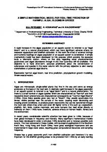
This is the smallest permissible period for the interrupts. It can be seen that the influence of bufsize on this value is comparatively small, and indeed if the interrupts are periodic there is no need for a buffer with more than one or two spaces, as the interrupts are either slower than or equal to the critical rate in which case there is never more than one unread character, or exceed this in which case a buffer of any size will eventually overflow. If however the interrupts are randomly distributed, then with a larger buffer we can replace this condition by two weaker ones. The constraints are that the interrupts must be far enough apart so that the interrupt can be serviced before the next interrupt occurs (this is true for any interrupt service routine), and that during a certain interval (which depends on the buffer size), no more interrupts can occur than can be processed in that interval. We give a practical application below where this constraint is much easier to satisfy than the “critical rate” constraint. The constraints derived from the program may be used, together with the timing information, the value of bufsize and a knowledge of the interrupt distribution function, either to determine that characters will not be lost (only possible if there is a lower bound on the inter-arrival time for interrupts), or to calculate the probability that this will happen. Suppose m = bufsize/2, and there are m characters in the buffer. Now if no more than m interrupts occur in time t, during which time m characters from the buffer are processed, at the end of this time the buffer will contain no more than m characters, and no characters will have been lost regardless of the distribution of the interrupts within this time. time taken to service m interrupts tI 6 6m + 1 time taken to process m characters tL 6 5m + 1 Therefore, maximum time to service m interrupts and to process m characters is given by t 6 11m + 2 Therefore, for random interrupts, we can say that provided no more than m interrupts occur during any interval of length 11m+2 then no characters will be lost. This can be used to determine the size of buffer required (since m = bufsize/2), or for an existing implementation, to determine the value of t and hence a constraint on the interrupt distribution which will ensure no characters are lost. For example, if interrupts come in bursts of not more than 10, randomly distributed in a period of at least 112 time units, then a buffer size of 20 will be sufficient to ensure that no characters are lost. 23

CPU

1M chars/sec Multiplexor

9600 baud

. . . Terminals Figure 3: A Terminal Multiplexer An example of such a system is a terminal multiplexer, connected to a number of terminals via serial lines and to a host computer via a high speed link (see Figure 3). The long term mean arrival rate of characters is limited by the baud rate of the serial lines, but characters may arrive from different terminals almost simultaneously, hence the need for a buffer. If the multiplexer link can deliver characters at a rate of one million per second, then the system would have to be capable of servicing and processing one character within one microsecond. However, serial lines of 9600 baud will deliver a maximum of 1 character per millisecond (approximately) per line, so within any one millisecond period there can be no more than 10 interrupts. The above analysis shows that provided an interrupts can be serviced in 1 microsecond, and a character processed within 99 microseconds, then a 20 character buffer will be sufficient to ensure that no characters are lost.

7

Recovering a specification

We have restructured the original program into the form shown in Figure 2, which has served to make its logic more explicit and has aided us in deriving timing constraints. However, although not executable, this program represents only a low level of abstraction. To recover a specification for the system we need to abstract away from the detail of the implementation. We present two approaches to this, the first an approach based on discovering and analysing loop invariants in the code as it stands. The second uses restructuring and inverse engineering to simplify the program before analysing the result. First we perform some low level abstraction from the program data structures. We can replace the external procedure write by its specification: if we regard the standard output as a sequence std out[. . . ] (as we did the program input) then we can write proc write(p var std out) ≡ std out := std out ++ hpi. We can replace the circular buffer buffer by a unbounded sequence buf. Since we know from Section 6 that the buffer will not overflow, making it larger will not affect the program. Characters are added to the buffer by appending to the tail, and removed from the head of the sequence. The 24

variables free, first and count are then redundant and can be removed. Setting time 0 equal to time before the procedure call and replacing the procedure call by its body, we get: PROG ≥ do if buf = hi then if input = hi then exit(1) elsf time < input[1][1] then time := input[1][1] fi fi; time 0 := time; while (input 6= hi ∧ time 0 > input[1][1]) do buf := buf ++ input[1][2]; input := tail(input); time > time + 6 od ch := buffer[first]; write(ch var stdout); std out := std out ++ buf [1]; buf := tail(buf ); time > time + 5 od; where we have abstracted away details of the assignment of values to time. Method 1: using loop invariants The program consists of two nested loops. We proceed by identifying the invariants and termination conditions for the loops. The loop invariant is a condition which is preserved by a loop throughout its execution. When the loop terminates therefore both the invariant and the termination condition are true; we can make use of this fact to find the specification of a loop. Consider first the inner while loop. We introduce new variables buf 0 , input0 , and immediately before the loop is entered assign buf 0 :=buf, input0 :=input. We can write the following invariant conditions on the assigned variables in the loop body: P buf = buf 0 ++ ji:=1 hinput0 [i][2]i ∧ input = input0 [j + 1 . .] ∧ time > time 0 + 6j where j is constrained by input[j][1] 6 time 0 , and in fact represents the number of iterations of the loop. The loop terminates when the condition input = hi ∨ time 0 < input[1][1] becomes true. Combining this with the invariant we get the following condition: input[j + 1 . .] ≡ hi ∨ time 0 < input0 [j + 1][1] We can therefore write the specification of the inner loop as j := µj 0 (j 0 > 0 ∧ input0 [j 0 + 1 . .] = hi ∨ time 0 < input0 [j 0 + 1][1]); P buf := buf 0 ++ ji:=1 hinput0 [i][2]i; input := input0 [j + 1 . .] time := time 0 .(time 0 > time 0 + 6j) where the first line is read as “j becomes equal to the smallest j 0 greater than or equal to 0 such that the remainder of the condition is true”. Substituting this specification for the inner loop gives: PROG ≥ do if buf = hi then if input = hi then exit(1) elsf time < input[1][1] then time := input[1][1] fi fi; 25

htime 0 := time, input0 := input, buf 0 := buf i; j := µj 0 (j 0 > 0 ∧ (input0 [j 0 + 1 . .] = hi ∨ time 0 < input0 [j 0 + 1][1])); P buf := buf 0 ++ ji:=1 hinput0 [i][2]i; input := input0 [j + 1 . .]; time := time 0 .(time 0 > time 0 + 6j + 5); std out := std out ++ hbuf [1]i; buf := tail(buf ) od; We now have a single loop. Restructuring the initial if statement makes explicit the termination condition for this loop: if buf = hi then if input = hi then exit(1) elsf time < input[1][1] then time := input[1][1] fi fi; ≈ if buf = hi ∧ input = hi then exit(1) fi; if buf = hi ∧ time < input[1][1] then time := input[1][1] fi; After the specification of the inner loop, we can say that time is greater than or equal to time of last input (interrupt) received. We can therefore eliminate the second if statement by using time 0 to record the time of the last interrupt. We can eliminate the new variables introduced in the last step by suitably ordering the statements, and abstract the second if statement to give: PROG ≥ do if buf = hi ∧ input = hi then exit(1) fi; if buf = hi then time > input[1][1] fi; time 0 := time; j := µj 0 (j 0 > 0 ∧ (input[j 0 + 1 . .] = hi ∨ time < input[j 0 + 1][1])); P buf := buf ++ ji:=1 hinput[i][2]i; if j > 0 then time 0 := input[j][1]; input := input[j + 1 . . ]; time > time 0 + 6j + 5; std out := std out ++ hbuf [1]i; buf := tail(buf ) fi od; We can now write down the invariant for the main loop of the program and hence derive the specification for the entire program. Again we use variables buf 0 , input0 , std out0 to record the initial values of variables before the loop is entered. In each iteration of the loop the buffer buf has j characters added to its end and one removed from its head. Also, std out has the first character from buf added to its end. input has j characters removed from its head. time is greater than or equal to the time of the last input (interrupt) processed. Therefore we can write down the following invariant: input = input0 [k + 1 . .] P ∧ buf = (buf 0 ++ ki:=1 hinput0 [i][2]i)[n + 1 . .] P ∧ std out = std out0 ++ (buf 0 ++ ki:=1 hinput0 [i][2]i)[1 . . n] ∧ time > input0 [k][2] + 11 The termination condition buf = hi ∨ input = hi is equivalent to the constraints (on k and n): input = hi ⇒ input0 [k + 1 . .] = hi

or k = `(input)

and buf = hi ⇒ (buf 0 ++

k X

hinput0 [1][2]i)[n + 1 . .] = hi

i:=1

26

or n = `(input 0 ) + `(buf 0 )

Substituting these conditions in the loop invariant, we arrive at the following: PROG ≥ hinput0 := input, buf 0 := buf , std out0 := std out, time 0 := timei; hk := `(input0 ), n := `(input0 ) + `(buf 0 )i; input := input0 [k + 1 . .]; buf := hi; P std out := std out0 ++ (buf 0 ++ ki:=1 hinput0 [i][2]i)[1 . . n]; time := time 0 .(time 0 > input0 [`(input0 )][1] + 11) Simplifying gives us the following specification: P`(input ) std out = std out0 ++ buf 0 ++ i=1 0 hinput0 [i][2]i; input := hi; buf := hi; time := time 0 .time 0 > input0 [`(input0 )][1] + 11 Method 2: transformation—changing the data structure We previously abstracted the program into the form PROG ≥ do if buf = hi then if input = hi then exit(1) elsf time < input[1][1] then time := input[1][1] fi fi; time 0 := time; while (input 6= hi ∧ time 0 > input[1][1]) do buf := buf ++ input[1][2]; input := tail(input); time := time 0 .(time 0 > time + 6) od ch := buffer[first]; write(ch var stdout); std out := std out ++ buf [1]; buf := tail(buf ); time := time 0 .(time 0 > time + 5) od; We are not really interested in the final value of time (which records the total time taken by the program), especially since this is dependent on the interrupt times provided in the input sequence. We are more interested in response times (the time taken to respond to each interrupt as it occurs) and these have already been covered by our analysis in Section 6. Therefore, in this section we will ignore the time variable and consider only the functional aspects of the program. In the inner while loop, characters are removed from the sequence input and appended to the sequence buf. If we define buf in = buf ++ π2 ∗ input where π2 (x, y) =DF y is the second projection, and π2 ∗ input is the sequence formed by concatenating the second elements of each element of input), and remove references to time, (so we consider only functional aspects of the program), we can rewrite the program as: PROG ≥ do if buf in = hi then exit(1) fi; std out := std out ++ hbuf in[1]i; buf in := tail(buf in) od; ≈ while buf in 6= hi do std out := std out ++ hbuf in[1]i; buf in := tail(buf in) od;

27

This approach will be generally applicable to programs using buffered input or output, and this single step results in a significant simplification. Introduce buf in0 = buf in, std out0 = std out before the loop is entered. The above is then equivalent to: hbuf in0 := buf in, std out0 := std outi; std out := std out0 ++ buf in0 ; buf in := hi; Now since buf in = buf ++ π2 ∗ input, we have hinput0 := input, buf 0 := buf , std out0 := std outi; std out := std out0 ++ buf 0 ++ π2 ∗ input0 ; buf := hi; input := hi; Thus we arrive at the following specification: std out := std out ++ buf ++ π2 ∗ input; input := hi; buf := hi which is identical to that obtained by the first method, with the exception that we have no specification of the elapsed time.

8

Conclusions

We have shown that the restructured program above in Figure 2 in Section 5.3 is an abstraction of the original program (with the assertion added). Trivially, the restructured program (NEW+ASSERT) is an abstraction of the same program without the assertion (NEW), since the removal of an assertion from any program is a refinement. NEW is a refinement of the specification (SPEC) derived in the previous section. So we have the following relationships: SPEC ≤ NEW

and

NEW+ASSERT ≤ ORIG+ASSERT ≤ ORIG

In Section 6.2 we derived conditions on the execution environment under which the assertion in NEW+ASSERT can be removed. Provided that these conditions are met, we can write NEW ≈ NEW+ASSERT and hence, by transitivity of refinement: SPEC ≤ ORIG Therefore, the derived specification correctly captures the behaviour of the original program provided the conditions on the distribution of interrupts are met. The derivation of these conditions or constraints hinged on the insertion of appropriate assertions into the program, in effect to “abstract away” some nonessential details. In this example this was a simple exercise, since the conditions under which incorrect program operation was possible could easily be identified. In a more complex program, it is likely that a significant amount of restructuring might be necessary before this would be possible. Similarly, the small number of paths through the program meant that timing information was easy to extract, and simple in form. “Real” programs typically have a large number of potential execution paths; automated assistance in the form of a tool which could extract timing information for all possible paths, and hence bounds on the execution time between to points in a program, would be valuable in the analysis of such programs. This study shows that using an appropriate model for interrupts we can represent interruptdriven programs within the (purely sequential) WSL language. With such models, the inverse engineering techniques of [44,48] can be applied to extract the specification of the original program. 28

Program transformations are sufficiently powerful to cope with these, often complex, models. Although a fairly large number of transformations are required to deal with these models, results from the case study indicate that these are used in a systematic way: moving assignments to time and calls to interrupt through the program to collect them together, unfolding and refolding where necessary. This suggests that much of the donkey work can be automated by a tool such as the Maintainer’s Assistant [13,51] and this is currently being investigated under a SMART 2 2 project at the Centre for Software Maintenance Ltd., and as part of a three-year SERC project at the University of Durham. 8.1

The Maintainer’s Assistant Project

In [50] we describe a practical program transformation system for reverse engineering which is based on our program transformation theory and has been used successfully with a number of IBM Assembler modules. The WSL language and transformation theory forms the basis of the “Maintainer’s Assistant” project [13,51] at Durham University and the Centre for Software Maintenance Ltd. which has developed a prototype transformation tool, implementing over six hundred transformations. The aim of the tool is to use program transformations to assist with program analysis, reverse engineering and general software maintenance. The tool consists of a structure editor, a browser and pretty-printer, a transformation engine and library of proven transformations, and a collection of translators for various source languages. The initial prototype of ReForm was developed as part of an Alvey project at the University of Durham [51]. This work on applying program transformation theory to software maintenance formed the basis for a joint research project between the University of Durham, Durham Software Engineering Ltd. and IBM UK Ltd. whose aim is to develop a tool which will interactively transform assembly code into high-level language code and Z specifications. We have been able to transform the assembler code to a high-level language representation, replace the “areas of store” by the data structures they implement (using transformations which change the data representation of a program), and then transform this high-level language version into a specification. A prototype translator has been completed and tested on sample sections of up to 80,000 lines assembler code, taken from very large commercial assembler systems. One particular module had been repeatedly modified over a period of many years until the control flow structure had become highly convoluted. Using the prototype translator and ReForm tool we were able to transform this into a hierarchy of (single-entry, single-exit) subroutines resulting in a module which was slightly shorter and considerably easier to read and maintain. The transformed version was hand-translated back into Assembler which (after fixing a single mis-translated instruction) “worked first time”. The ReForm tool (Reverse Engineering through FORmal Methods), is designed to automate much of the process of transforming code into specifications and specifications into code. This process can never be completely automated—there are many ways of writing the specification of a program, several of which may be useful for different purposes. So the tool must work interactively, with the tedious checking and manipulation carried out automatically, while the maintainer provides high-level “guidance” to the transformation process. In the course of the development of the prototype, we have been able to capture much of the knowledge and expertise that we have developed through manual experiments and case studies with earlier versions of the tool, and incorporate this knowledge within the tool itself. For example, restructuring a regular action system (a collection of gotos and labels) can now be handled completely automatically through a single transformation. ReForm can also be used as a software development system (but this is not the focus of this paper): starting with a high-level specification expressed in set-theory and logic notation (similar 2

Small Firms Merit Award for Research and Technology

29

to Z or VDM [24]), the user can successively transform it into an efficient, executable program. Transformations are themselves coded in an extension of WSL called METAWSL: in fact, much of the code for the prototype is written in WSL, and this makes it possible to use the system to maintain its own code. The FermaT project is a complete redevelopment of the Maintainer’s Assistant prototype to build an industrial strength CASE tool for reverse engineering, software maintenance and program understanding.

Acknowledgements The research described in this paper has been partly a Department of Trade and Industry SMART award, partly by Durham Software Engineering Ltd., and partly by SERC3 project “A Proof Theory for Program Refinement and Equivalence: Extensions”.

References [1] J. R. Abrial, S. T. Davis, M. K. O. Lee, D. S. Neilson, P. N. Scharbach & I. H. Sørensen, The B Method, BP Research, Sunbury Research Centre, U.K., 1991. [2] J. Arsac, “Transformation of Recursive Procedures,” in Tools and Notations for Program Construction, D. Neel, ed., Cambridge University Press, Cambridge, 1982, 211–265. [3] R. J. R. Back, Correctness Preserving Program Refinements, Mathematical Centre Tracts #131, Mathematisch Centrum, Amsterdam, 1980. [4] R. Balzer, “Transformational Implementation: An Example,” IEEE Trans. Software Eng. SE-7 (Jan., 1981), 3–14. [5] R. Barstow, H. E. Shrobe & E. Sandwall, Interactive Programming Environments, McGraw-Hill, New York, NY, 1984. [6] F. L. Bauer & The CIP Language Group, The Munich Project CIP, Volume I: The Wide Spectrum Language CIP-L, Lect. Notes in Comp. Sci. #183, Springer-Verlag, New York–Heidelberg–Berlin, 1985. [7] F. L. Bauer, B. Moller, H. Partsch & P. Pepper, “Formal Construction by Transformation—Computer Aided Intuition Guided Programming,” IEEE Trans. Software Eng. 15 (Feb., 1989). [8] F. L. Bauer & The CIP System Group, The Munich Project CIP, Volume II: The Program Transformation System CIP-S, Lect. Notes in Comp. Sci. #292, Springer-Verlag, New York–Heidelberg–Berlin, 1987. [9] F. L. Bauer & H. Wossner, Algorithmic Language and Program Development, Springer-Verlag, New York–Heidelberg–Berlin, 1982. [10] R. Bird, “Lectures on Constructive Functional Programming,” in Constructive Methods in Computing Science, M. Broy, ed., NATO ASI Series #F55, Springer-Verlag, New York–Heidelberg–Berlin, 1989, 155–218. [11] J. M. Boyle, “LISP To FORTRAN—Program Transformation Applied,” in Program Transformation and Programming Environments Report on a Workshop directed by F. L. Bauer and H. Remus, P. Pepper, ed., Springer-Verlag, New York–Heidelberg–Berlin, 1984, 199–222. [12] M. Broy, R. Gnatz & M. Wirsing, “Semantics of Nondeterminism and Noncontinuous Constructs,” in Program Construction, G. Goos & H. Hartmanis, eds., Lect. Notes in Comp. Sci. #69, Springer-Verlag, New York–Heidelberg–Berlin, 1979, 563–592. [13] T. Bull, “An Introduction to the WSL Program Transformer,” Conference on Software Maintenance 26th–29th November 1990, San Diego (Nov., 1990).

3

The Science and Engineering Research Council

30

[14] R. M. Burstall & J. A. Darlington, “A Transformation System for Developing Recursive Programs,” J. Assoc. Comput. Mach. 24 (Jan., 1977), 44–67. [15] A. Church, “The Calculi of Lambda Conversion,” Annals of Mathematical Studies 6 (1941). [16] R. B. K. Dewar, E. Schonberg & J. T. Schwartz, “Higher Level Programming: Introduction to the Use of the Set-theoretic Programming Language SETL,” Courant Institute of Mathematical Science, New York University, Technical Report, New York, 1981. [17] E. W. Dijkstra, A Discipline of Programming, Prentice-Hall, Englewood Cliffs, NJ, 1976. [18] E. Engeler, Formal Languages: Automata and Structures, Markham, Chicago, 1968. [19] M. S. Feather, “A Survey and Classification of Some Program Transformation Techniques,” in Proceedings of the IFIP TC2/WG2 Working Conference on Program Specification and Transformation, L. G. L. T. Meertens, ed., Elsevier Science Publishers, Amsterdam, 1987, 165–196. [20] M. S. Feather, “A System for Assisting Program Transformation,” Trans. Programming Lang. and Syst. 4 (Jan. 1982), 1–20. [21] S. F. Fickas, “Automating the Transformational Development of Software,” University of California, Ph.D. dissertation, Irvine, 1982. [22] S. F. Fickas, “Automating the Transformational Development of Software,” IEEE Trans. Software Eng. 11 (Nov., 1985). [23] C. A. R. Hoare, I. J. Hayes, H. E. Jifeng, C. C. Morgan, A. W. Roscoe, J. W. Sanders, I. H. Sørensen, J. M. Spivey & B. A. Sufrin, “Laws of Programming,” Comm. ACM 30 (Aug., 1987), 672–686. [24] C. B. Jones, Systematic Software Development using VDM , Prentice-Hall, Englewood Cliffs, NJ, 1986. [25] C. B. Jones, K. D. Jones, P. A. Lindsay & R. Moore, mural: A Formal Development Support System, Springer-Verlag, New York–Heidelberg–Berlin, 1991. [26] C. R. Karp, Languages with Expressions of Infinite Length, North-Holland, Amsterdam, 1964. [27] D. E. Knuth, “Structured Programming with the GOTO Statement,” Comput. Surveys 6 (1974), 261–301. [28] B. Krieg-Bruckner, “The PROSPECTRA Methodology of Program Developments”,” North-Holland, IFIP/IFAC Working Conference on Hardware and Software for Real Time Processes, Warsaw, Amsterdam, 1988. [29] M. E. Majester, “Limits of the ‘Algebraic’ Specification of Abstract Data Types,” SIGPLAN Notices 12 (Oct., 1977), 37–42. [30] C. C. Morgan, “The Specification Statement,” Trans. Programming Lang. and Syst. 10 (1988), 403–419. [31] C. C. Morgan, Programming from Specifications, Prentice-Hall, Englewood Cliffs, NJ, 1994, Second Edition. [32] C. C. Morgan, K. Robinson & Paul Gardiner, “On the Refinement Calculus,” Oxford University, Technical Monograph PRG-70, Oct., 1988. [33] D. J. Mostow, “Machanical Transformation of Tasks Heuristics into Operational Procedures,” CarnegieMellon University, Ph.D. dissertation, Rep. CMU-CS-81-113, Pittsburg, Pa., 1981. [34] M. Neilson, K. Havelund, K. R. Wagner & E. Saaman, “The RAISE Language, Method and Tools,” Formal Aspects of Computing 1 (1989), 85–114 . [35] H. Partsch, “The CIP Transformation System,” in Program Transformation and Programming Environments Report on a Workshop directed by F. L. Bauer and H. Remus, P. Pepper, ed., Springer-Verlag, New York–Heidelberg–Berlin, 1984, 305–323. [36] H. Partsch & R. Steinbr¨ ugen, “Program Transformation Systems,” Computing Surveys 15 (Sept., 1983).

31

[37] P. Pepper, “A Study on Transformational Semantics,” in Program Construction, G. Goos & H. Hartmanis, eds., Lect. Notes in Comp. Sci. #69, Springer-Verlag, New York–Heidelberg–Berlin, 1979, 322–405. [38] C. T. Sennett, “Using Refinement to Convince: Lessons Learned from a Case Study,” Refinement Workshop, 8th–11th January, Hursley Park, Winchester (Jan., 1990). [39] D. R. Smith, “KIDS: A Semiautomatic Program Development System,” IEEE Trans. Software Eng. 16 (1990), 1024–1043. [40] D. Taylor, “An Alternative to Current Looping Syntax,” SIGPLAN Notices 19 (Dec., 1984), 48–53. [41] T. Teitelbaum & T. Reps, “The Cornell Program Synthesizer,” Comm. ACM 24 (Sept., 1981), 563–573. [42] M. Ward, “Proving Program Refinements and Transformations,” Oxford University, DPhil Thesis, 1989. [43] M. Ward, “Derivation of a Sorting Algorithm,” Durham University, Technical Report, 1990, hhttp: // www. dur. ac. uk/ ∼dcs0mpw/ martin/ papers/ sorting-t.ps.gzi. [44] M. Ward, “Specifications and Programs in a Wide Spectrum Language,” Submitted to J. Assoc. Comput. Mach., 1991. [45] M. Ward, “Foundations for a Practical Theory of Program Refinement and Transformation,” Durham University, Technical Report, 1994, hhttp: // www. dur. ac. uk/ ∼dcs0mpw/ martin/ papers/ foundation2t.ps.gzi. [46] M. Ward, “The Largest True Square Problem—An Exercise in the Derivation of an Algorithm,” Durham University, Technical Report, Apr., 1990. [47] M. Ward, “Iterative Procedures for Computing Ackermann’s Function,” Durham University, Technical Report 89-3, Feb., 1989, hhttp: // www. dur. ac. uk/ ∼dcs0mpw/ martin/ papers/ ack-t.ps.gzi. [48] M. Ward, “Abstracting a Specification from Code,” J. Software Maintenance: Research and Practice 5 (June, 1993), 101–122, hhttp: // www. dur. ac. uk/ ∼dcs0mpw/ martin/ papers/ prog-spec.ps.gzi. [49] M. Ward, “Derivation of Data Intensive Algorithms by Formal Transformation,” IEEE Trans. Software Eng. 22 (Sept., 1996), 665–686, hhttp: // www. dur. ac. uk/ ∼dcs0mpw/ martin/ papers/ sw-alg.ps.gzi. [50] M. Ward & K. H. Bennett, “A Practical Program Transformation System For Reverse Engineering,” Working Conference on Reverse Engineering, May 21–23, 1993, Baltimore MA (1993), hhttp://www.dur. ac. uk/ ∼dcs0mpw/ martin/ papers/ icse.ps.gzi. [51] M. Ward, F. W. Calliss & M. Munro, “The Maintainer’s Assistant,” Conference on Software Maintenance 16th–19th October 1989, Miami Florida (1989), hhttp: // www. dur. ac. uk/ ∼dcs0mpw/ martin/ papers/ MA-89.ps.gzi. [52] D. S. Wile, “Program Development: Formal Explanations of Annotations,” Comm. ACM 26 (1983), 902– 911. [53] H. Wossner, P. Pepper, H. Partsch & F. L. Bauer, “Special Transformation Techniques,” in Program Construction, G. Goos & H. Hartmanis, eds., Lect. Notes in Comp. Sci. #69, Springer-Verlag, New York–Heidelberg–Berlin, 1979, 290–321.

32