Journal of Oceanography, Vol. 66, pp. 291 to 297, 2010
Inverse Estimation of Drifting-Object Outflows Using Actual Observation Data S HIN’ICHIRO KAKO1*, ATSUHIKO ISOBE 1, SATOQUO SEINO2 and AZUSA KOJIMA3 1
Center for Marine Environmental Studies, Ehime University, Bunkyo-cho, Matsuyama 790-8577, Japan 2 Urban and Environmental Engineering, Faculty of Engineering, Kyushu University, Fukuoka 819-0395, Japan 3 Japan Environmental Action Network, Tokyo 185-0021, Japan (Received 3 July 2009; in revised form 19 November 2009; accepted 20 November 2009)
The present study attempts to establish a scientifically reliable method capable of computing the drifting-object sources and their outflows. First, the temporal variability of the drifting-object amount is investigated every two months on a beach west of Japan, where various source regions are anticipated because of spatiotemporally variable northeastward ocean currents over the East China Sea. Next, in order to specify drifting-object sources, two-way particle tracking model (PTM) experiments are carried out using simulated ocean currents and leeway drift estimated from QuikSCAT/Seawinds wind data. Finally, an inverse method with a Lagrange multiplier is applied to estimate drifting-object outflows at each source on the basis of the two-way PTM results and beach surveys. Accuracy of object-source identification using the two-way PTM is validated by comparing disposable-lighter sources suggested by phone numbers printed on the lighter surface with those computed by the model. In order to examine the reliability of the inverse estimation, the number of plastic-bottle caps found in actual beach surveys is compared with that computed using a forward in-time PTM during the same period of actual beach surveys, over which the outflows obtained using the inverse method are given at each source in the model.
Keywords: ⋅ East China Sea, ⋅ two-way particle tracking model, ⋅ beach survey, ⋅ inverse method.
scribed later in Subsection 2.3) which is able to evaluate whether source candidates are statistically significant or not. Their approach is capable of seeking sources of objects drifting on the sea surface over the course of several months, which are much longer than the period taken by the previous PTMs (e.g., Batchelder, 2006) used to find object sources. For the first time, we employ this approach to find the sources of the objects found on an actual beach in the present study. However, the amount of objects flowing out from each source each month cannot be directly specified by the PTM alone due to the limited number of observations. To solve this underdetermined problem of quantifying the object outflows (i.e., number of released objects) from each source identified using the above-mentioned two-way PTM, we next attempt to solve an inverse problem using the results of actual beach surveys and two-way PTM as the data and model constraints, respectively. Explicitly, in the present study, the two-way PTM demonstrates the locations and times at which drifting objects are released,
1. Introduction One of the things of interest in walking on beaches is to find drifting objects (bottles, fishery floats, and so forth) originating from foreign countries, although the excessive drifting-object accumulation on the beaches may give rise to an environmental issue as beach litter. We often imagine object-source countries by looking at foreign lettering printed on the object surface. The present physical oceanographic study provides us with a procedure to convert this imagination into identification using an inverse method with a numerical ocean-circulation model, particle-tracking models (hereinafter, PTMs), satellite-derived wind data, and field surveys to count the number of drifting objects on a beach. To seek drifting-object sources, Isobe et al. (2009) recently proposed a two-way PTM approach (briefly de* Corresponding author. E-mail:
[email protected] Copyright©The Oceanographic Society of Japan/TERRAPUB/Springer
291
(a)
(b)
Bohai Sea
Yellow Sea
East China Sea
Fig. 1. Disposable-lighter sources derived from the two-way PTM experiments (a) and those derived from beach surveys at the Hassakubana beach (b). The location of the beach in Goto Islands is shown in the inset map in the panel (a). The rotated square in the panel indicates the model domain. When the phone numbers printed on the lighters suggested sources far from the coasts, these sources were removed from the panel (b) for comparison with panel (a).
while object-outflows from each source are computed using the inverse method. It is anticipated that our approach is capable of specifying the sources and outflows of fish eggs, larvae, marine pollutants, and beach litter whose condition has been widely recognized as a serious environmental issue on beaches surrounding the East Asian marginal seas (Seino et al., 2009). 2. Methods 2.1 Beach surveys The number of drifting objects was counted on an actual beach before computing object sources and outflows in the two-way PTM. Since the details of this “beach survey” are published in Seino et al. (2009), a brief explanation of the experimental design is presented below. The Hassakubana beach (the inset map in Fig. 1(a)) at Goto Islands was chosen as the fixed station for this survey because various source countries are expected for drifting objects carried by spatiotemporally variable northeastward ocean currents over the actual East China Sea (Isobe, 2008). In addition, the Hassakubana beach has the advantage of good accessibility, making it possible to convey many of the participants of these surveys onto the beach. Furthermore, it is also expected that the drifting-object number counted on the beach is representa292
S. Kako et al.
tive of the Goto islands because this beach is located neither within a narrow channel nor behind a headland, but is facing the East China Sea directly. Disposable lighters were chosen as drifting-object items in this experiment because the phone numbers usually printed on the lighters are useful for identifying the areas from which they probably flowed out (Fujieda and Kojima, 2006). In addition, plastic-bottle caps with lettering information are chosen as items because the large number of caps found on the beach is convenient for computing the outflows at the sources. The beach surveys had been carried out once every two months for the years 2007 through 2008 (7 times in total; Sept. 16–17, Nov. 4–5, 2007, Jan. 19–20, Mar. 9– 10, May 10–11, July 12–13, and Sept. 13–15, 2008); 20– 30 voluntary citizens and researchers took part in each beach survey and the above two items on the 350-m long stretch of beach were all retrieved and counted over the course of two days. In the present study, we regard the drifting-object number counted on the day of each beach survey (except for the first survey) as the total number of objects reaching the Hassakubana beach over the course of two months (i.e., the interval between beach surveys). The first survey result is not used for the following analyses because the object number obtained in the first survey is the cumulative one before September 2007. We
might underestimate the “true” number of objects reaching the beach because of neglecting “re-drifting” objects which return to the ocean from the beach. Although there is no way of knowing, at the present time, the accurate number of re-drifting objects during the two months, we carry out a numerical model experiment to validate object sources and outflows obtained in the present application (see Section 3). 2.2 Models A hydrographic model and PTM were first constructed to compute drifting-object behavior over the East China Sea shelf. The hydrographic model used here is based on that in Chang and Isobe (2003) using the Princeton Ocean Model (POM; Blumberg and Mellor, 1987). The model domain covering the whole of the East China and Yellow Seas (see Fig. 1 for its area) is divided into 1/12-degree grid boxes in both latitude and longitude, and 16σ-layers vertically. The bottom topography data (ETOPO5) with a 5-minute resolution are provided by the National Geophysical Data Center. The inflowoutflow conditions at the open boundaries, winds, heat and freshwater fluxes are given to the model using the long-term monthly averaged values given by Chang and Isobe (2003). To spin-up the POM, the monthly climatological wind stress of the Comprehensive OceanAtmosphere Data Set with a two-degree resolution is imposed on the surface, using a stability-independent drag coefficient in line with Large and Pond (1981). After the 7-year spin-up computation, the POM is driven using daily wind speed data observed by QuikSCAT/Seawinds (provided by the Jet Propulsion Laboratory; http:// podaac.jpl.nasa.gov/) in specific years. Missing values are recovered by applying the optimum interpolation method used in Kako and Kubota (2006). The accuracy of our hydrographic model has already been validated in Chang and Isobe (2003). For example, the modeled Changjiangderived fresh water distribution on the sea surface is fairly consistent with the observed one, so it is likely that the modeled surface currents are sufficiently accurate to reproduce drifting-object motion. The PTM in the present study is the same as that used in Isobe et al. (2009). The modeled particles in the PTM are carried by ambient surface currents (at 0.3-m depth) computed in the hydrographic model in conjunction with random-walk processes. In the present PTM application, the particle location [X = (x, y)] at the time t + ∆t, where ∆t is the time increment of the hydrographic model, is computed as X t + ∆t = X t + U∆t +
1 ∂U 2 U ⋅ ∇HU + ∆t + R 2 Kh ∆t (i, j), 2 ∂t
(1)
where U [=(u, v)] and Kh are the current vector and diffusivity computed in the hydrographic model at the specific depth, and i and j denote the unit vectors in the zonal (x) and meridional (y) directions, whereas R represents a random number generated at each time step with the average and standard-deviation of 0.0 and 1.0, respectively. In computing the motion of the drifting disposable lighters exposed partly in the air, the influence of the drag force exerted directly by winds (i.e., leeway drift) should be added to the ambient currents in PTMs. To incorporate the leeway drift into the PTM algorithm, we use Richardson’s (1997) relationship between the wind speed (W) and leeway drift (V) as follows: V=
ρ a Cda Aa , ρ w Cdw Aw
(2 )
where ρa (ρw) is the air (seawater) density, Cd a (Cd w) is the drag coefficient for the lighters in the air (seawater), respectively, and Aa (Aw) denotes the horizontally projected area of the lighters. We use values ρa/ρw = 1.15 × 10⁻³ and Cda/Cdw = 1.0 in the present application, assuming that Reynolds numbers in both air and water are less than the critical values at which the drag coefficient suddenly decreases. Constant Aa/Aw values are however unlikely to be appropriate for expressing the various status of drifting lighters in the actual ocean. In the present model, the ratio (Aa/Aw) changes from 1/300 to 1, although the choice of the denominator 300 is somewhat arbitrary but shall be used to express the situation in which lighters with air chambers are unlikely to sink completely beneath the sea surface. The drifting processes of plasticbottle caps are unaffected by the leeway drift because they are carried mostly beneath the sea surface. 2.3 Two-way PTM and inverse method A two-way PTM and an inverse method using a Lagrange multiplier are adopted to identify the object sources and outflows. The capability of the two-way PTM to identify object sources has already been presented in Isobe et al. (2009), so a brief explanation of this procedure is described below. First, backward-in-time PTM experiments are carried out to determine the object-source candidates. In these backward-in-time PTM experiments, ten thousand particles placed at the Hassakubana beach on the same date as the beach surveys are carried by modeled ambient currents (and leeway drift) with directions reversed in sign for both horizontal current components. The object source candidates are determined monthly by recording the coasts where the particles reach over the course of each month. However, in general, the source identification using backward-in-time PTMs is unreliable because object motion
Inverse Estimation of Drifting-Object Outflows Using Actual Observation Data
293
includes irreversible random-walk processes which cannot be reproduced “backward” in time. Thereby, using forward-in-time PTMs with the ambient currents computed in the original hydrographic model, ten thousand particles are thereafter released from each source candidate detected in the foregoing backward-in-time PTM to examine whether or not each object source candidate is statistically significant. On each day of the actual beach surveys, if the Hassakubana beach is located at a place closer than two times the standard deviation of the distances between particle positions and their averaged one, the object sources from which these particles were released are considered to be significant at the 95% confidence level. Second, object outflows at each source detected in the above two-way PTM are computed using an inverse method. The relationship between the number (z; a constant in each beach survey) of the objects reaching the Hassakubana beach over the course of two months and outflows (f; a row vector) at various sources is expressed as:
(f
M −l , f2M − l , f3M − l , K, f NM− 2 , f NM−1 , f NM 1
g1 g2 g3 = z, . . g N × (l +1)
)
(3)
where the subscripts represent sources (N; the total number), and the superscripts denote the month in which objects flow out from each source, and M means the month when a beach survey is conducted to obtain z; it is assumed that the observed number z is derived from the outflows up to l months before. M-, and l are different by beach surveys (from 8 to 12 are chosen for l in the present application) because the periods taken for almost all the objects to cross the East China Sea are different by seasons. A column vector g denotes weights of outflows at each source in determining z, and depends on the oceancurrent (and leeway-drift) contribution to drifting object behavior over the East China Sea shelf. This vector g is invariant in each survey computation because ocean currents and winds over the East China Sea must be uniquely determined to convey the number z of drifting objects observed at the Hassakubana beach. Before obtaining the outflow vector f in Eq. (3), we have to compute the column vector g. However, Eq. (3) involves apparently the underdetermined problem of obtaining the vector g, thus we need first to compute the vector g using the numerical model experiment independ294
S. Kako et al.
ent of the actual beach surveys. The row vector f and a constant z in this equation are replaced with a symmetric matrix and column vector, respectively, as follows,
1000 10000 10000 L 10000 g1 10000 1000 10000 L 10000 g2 10000 10000 1000 L 10000 g3 M M M M O M 10000 10000 10000 L 1000 g N × (l +1) H1 H2 = H3 . M H N × (l +1)
( 4)
The above equation means that 10,000 particles are given to all sources except for a single source (see symmetric components) from which the 1,000 particles are released in the forward-in-time PTM experiment. To obtain the symmetric matrix on the left-hand side of the equation, forward in-time PTMs are conducted repeatedly for the number of symmetric components. These component values in the matrix were chosen arbitrarily, but gave a column vector H (right-hand side) of which components represent different numbers (various H values) of particles reaching the Hassakubana beach simulated in the forwardin-time PTM experiments with various f combinations. The column vector g can be obtained directly by substituting the symmetric matrix and H vector obtained in N × (l + 1)-time experiments into Eq. (4). Next, the unknown outflow vector f in Eq. (3) is obtained using the known vector g computed by the above procedure in conjunction with z observed actually on the Hassakubana beach. However, this is still an underdetermined problem, and so Eq. (3) is solved using an unknown Lagrange multiplier (λ). A priori information required in this inverse method is to minimize a vector D defined as
(
)
D = f1M − l e1 , f2M − l e2 , f3M − l e3 , K, f NM e N ,
(5)
where e (=T/L) means the “efficiency” of the object transport between the source and receptor (i.e., the Hassakubana beach). T denotes the time elapsed between the object release at a source and observation at the receiving end, and L represents the distance between the source and receptor. This information (Eq. (5)), choosing the most efficient combination of the source outflows, is
combined with the constraint condition (Eq. (3)) using the Lagrange multiplier as follows.
φ = D ⋅ D T + λ ( z − f ⋅ g).
(6 )
Minimizing φ with respect to the outflows (each component of f) yields
(f
M −l , f2M − l , f3M − l , K, f NM 1
=
)
g N × (l +1) λ g1 g2 g3 2 , 2 , 2 , K, 2 . 2 e1 e2 e3 e N × (l +1)
(7) month
Substituting the above f values into Eq. (3), we obtain
λ = 2z
N × ( l +1)
∑
i =1
2
gi . ei
(8)
Thereafter, we are able to compute outflows (f) by substituting (8) into each component of (7). The outflows throughout a year are computed using z values observed every two months on the Hassakubana beach (6 times in total). In addition, the outflows from Japan, Korea, and China are computed separately by using the number of objects on which characters of these three countries were printed; in fact the beach-survey results show that almost all the drifting objects originate from these countries. Explicitly, the above inverse estimation is repeated 18 times in total in the present application. 3. Results and Discussion Results of the two-way PTM experiments to find disposable-lighter sources demonstrate that model sources (Fig. 1(a)) are indeed consistent with those suggested by the phone numbers (Fig. 1(b)) printed on the lighters’ surface; all sources detected in the 6-time two-way PTMs (beach surveys) are superimposed in the left (right) panel. In particular, neither the two-way PTM-experimental results nor the observational results have sources west of the Yellow and Bohai Seas. Thus, modeled currents, the estimated leeway drift, and two-way PTM are capable of identifying the object sources in the actual ocean. Next, using the inverse method in conjunction with the beach survey results, we estimate the outflows of plastic-bottle caps at each source specified by the two-way PTM experiments in the same manner as those for the lighters. The results of the beach surveys show a remarkable seasonal variability in plastic-bottle cap numbers (Fig. 2); for instance, a large number of the caps arrive during the months September through January, and the number in each month thereafter continued to be small
Fig. 2. Seasonal variability of plastic-bottle cap numbers at the Hassakubana beach in Goto Islands. The three tone patterns are used for caps with characters of three countries shown in the upper right of the figure. The digits “9–11” in the abscissa, for instance, denotes the cap-number difference between the numbers found in September and November surveys, and indicates the number of caps arriving in the course of this period.
until the next September. Figure 3 shows the plastic-bottle cap outflows computed using the inverse method. The bar heights denote the number of plastic-bottle caps originating from the sources (the digits are normalized using the number (58) of Japanese caps found in the actual beach survey in November 2008), and the colors denote the month when the caps flow out from each source. Note that the coasts without color bars do not always mean no outflows, but may mean that none of the caps originating from these coasts in fact reach the Hassakubana beach. In spite of a lot of caps flowing out from Taiwan and the Changjiang river mouth in the summer (Fig. 3), the cap numbers with Chinese (in the present study including Taiwanese) characters were not so different from those with Korean and Japanese characters at the Hassakubana beach (Fig. 2), so it is reasonable to suppose that caps from China reach Japanese coasts less easily than those from Japan and Korea. To validate the inverse estimation in the present study, the particle outflows computed with the inverse method are placed in same months/sources as in Fig. 3 using the forward-in-time PTM, and thereafter the numbers of particles reaching the modeled Hassakubana beach during the period of the beach surveys are compared with those obtained in the actual beach surveys (Fig. 4). It is noted that the modeled particles released from the sources must reach the Hassakubana beach during the month when the particles are released from the Hassakubana beach in the backward-in-time PTM for finding the source candidates. The particles are therefore removed in the model
Inverse Estimation of Drifting-Object Outflows Using Actual Observation Data
295
when they reach the beach before this month, or when they still drift in the model ocean after this month. Figure 4 demonstrates that the seasonality of plastic-bottle cap numbers is well reproduced in the model in spite of neglecting the re-drifting processes of drifting objects, and that this inverse method combined with beach surveys is capable of identifying object sources, and of estimating object outflows from the sources. It is found, however, that the model results are slightly smaller than the beach survey results over the observation period. Although an in-depth examination is required in order to be conclusive, a priori information to minimize the vector D (Eq. (5)) may lead to this underestimation because of drifting particles not satisfying this information to reach the Hassakubana beach in the model. 4. Summary The objective of the present study was to establish a scientifically reliable method capable of computing drifting-object sources and their outflows. First, we counted the number of drifting objects (disposable lighters and plastic-bottle caps) every two months on the Hassakubana beach, and investigated phone numbers printed on the lighters’ surface to suggest their source countries. Second, a hydrographic model and two-way PTM using simulated ocean currents and leeway drift estimated from QuikSCAT/Seawinds wind data were constructed to com296
S. Kako et al.
numbers of plastic-bottle caps
Fig. 3. Plastic-bottle cap outflows from each source detected in the inverse method.
Fig. 4. Comparison between numbers of plastic-bottle caps reaching the Hassakubana beach in the model and those found in the beach surveys. The meaning of digits like “9– 11” is the same as that in Fig. 2.
pute drifting-object behavior over the East China Sea shelf. The disposable-lighter sources identified in the twoway PTM experiments are indeed consistent with those suggested by the phone numbers. Third, an inverse method using the PTM and beach-survey results was applied to estimate the plastic-bottle cap outflows at sources, and
was validated in a forward in-time PTM. The seasonality of the plastic bottle caps reaching the Hassakubana beach in the model, where cap outflows derived from the inverse method are given to each source, is indeed consistent with the results of the beach surveys. We are applying the reliable system developed in the present study to beach litter whose condition has been widely recognized as a serious environmental issue on beaches surrounding the East Asian marginal seas (Seino et al., 2009). The system provides us with beach-litter sources which will be available for public awareness to reduce its occurrence, and with a beach-litter amount forecast which will enable efficient clean-up work on beaches. Acknowledgements The authors express their sincere thanks to Profs. Masahisa Kubota and Takeshi Matsuno, and two anonymous reviewers for their critical comments. This research was supported by the Global Research Fund (D-071) of the Ministry of the Environment, Japan. References Batchelder, H. P. (2006): Forward-in-time/Backward-in-timetrajectory (FITT/BITT) modeling of particles and organisms in the coastal ocean. J. Atmos. Oceanic Technol., 23, 727–741. Blumberg, A. F. and G. L. Mellor (1987): A description of a three-dimensional coastal ocean circulation model. p. 1–
16. In Three-dimensional Coastal Ocean Models, Coastal Estuarine Sci., Vol. 4, ed. by N. S. Heaps, AGU, Washington, D.C. Chang, P.-H. and A. Isobe (2003): A numerical study on the Changjiang diluted water in the Yellow and East China Seas. J. Geophys. Res., 108(C9), doi:10.1029/2002JC00179. Fujieda, S. and A. Kojima (2006): Estimation of the sources of marine liter drifted on the coast of East Asia. Journal of Coastal Zone Studies, 18, 15–22 (in Japanese with English abstract). Isobe, A. (2008): Recent advances in ocean circulation research on the Yellow and East China Sea shelves. J. Oceanogr., 64, 569–584. Isobe, A., S. Kako, P.-H. Chang and T. Matsuno (2009): Twoway particle tracking model for specifying sources of drifting objects: application to the East China Sea shelf. J. Atmos. Oceanic Technol., 26, 1672–1682. Kako, S. and M. Kubota (2006): Relationship between an El Nino event and the interannual variability of significant wave heights in the North Pacific. Atmosphere-Ocean, 44, 377–395. Large, W. G. and S. Pond (1981): Open ocean momentum flux measurement in moderate to strong winds. J. Phys. Oceanogr., 11, 324–336. Richardson, P. L. (1997): Drifting in the wind: leeway error in shipdrift data. Deep-Sea Res., 44(11), 1878–1903. Seino, S., A. Kojima, H. Hinata, S. Magome and A. Isobe (2009): Multi-Sectoral research on East China Sea beach litter based on oceanographic methodology and local knowledge. Journal of Costal Research, 2, 56, 1289–1292.
Inverse Estimation of Drifting-Object Outflows Using Actual Observation Data
297