Inverting geophysical data with Markov chain Monte

Inverting geophysical data with Markov chain Monte Carlo methods and parameter space reduction Nicholas Reid

A thesis submitted for the degree of Master of Science at The University of Queensland in 2018 School of Mathematics and Physics

I give consent for copies of this report to be made available, as a learning resource, to students enrolled at The University of Queensland.

Abstract Inverse problems in geophysics allow us to gauge parameters we cannot directly observe. A desire to quantify uncertainty of the inverted parameters requires formulating the problem as one of statistical inversion - the associated forward problem is a model which maps the parameters to some observable output. Recasting the parameters and model predicted output as random variables, Markov chain Monte Carlo (MCMC) sampling methods can be used to recover a probability density function over the parameter space. If the intent is to recover spatially distributed parameters, such as hydraulic conductivity or electrical resistivity fields, the challenge faced by the sampling method of exploring the high dimensional parameter space in finite time soon becomes impractical if we desire a parameter field that is at least somewhat informative. We consider a method of parameter space reduction in the continuous setting where the parameter field is approximated by a linear combination of basis functions. The basis functions are produced offline leaving only their coefficients for the MCMC process to recover. The dimensionality of the parameter space becomes a nominal variable which dictates the desired level accuracy of the recovered parameter field. Carrying out the inversion in the continuous setting allows an unstructured mesh to be used for discretisation and facilitates mesh independence. The numerical examples include two-dimensional hydraulic conductivity and electrical resistivity inversion problems. Thesis Supervisor: Lutz Gross Title: Associate Professor, Computational Geophysics and Modelling, School of Earth and Environmental Sciences

Publications included in this thesis No publications included.

Submitted manuscripts included in this thesis No manuscripts submitted for publication.

Other publications during candidature No other publications.

Statement of parts of the thesis submitted to qualify for the award of another degree No works submitted towards another degree have been included in this thesis.

Research involving human or animal subjects No animal or human subjects were involved in this research.

Acknowledgements A big thankyou to my thesis supervisor Associate Professor Lutz Gross of the School of Earth and Environmental Sciences at The University of Queensland who met with me once a week after hours to accommodate my work commitments for over a year. I could not have completed my thesis without his constant assistance and invaluable advice. He always knew what to try next when I was stuck and offered a number of improvements to various aspects of my research. I would like to thank Dr Andrea Codd also of the School of Earth and Environmental Sciences at The University of Queensland for her assistance with deriving the gradient of the Greedy Sampling algorithm, and Junpeng Lao from PyMC3-discourse for his assistance with setting up the Bayesian statistical model. A big thanks to my friends and family for their patience and support over the past year and a bit. And my girlfriend Gracie, who was always so accommodating of the late nights and weekends I spent working on my thesis, I’m so appreciative of her unquestioning support.

Financial support No financial support was provided to fund this research.

Keywords Statistical inversion, model reduction, parameter space reduction, optimisation, MCMC

Australian and New Zealand Standard Research Classifications (ANZSRC) ANZSRC code: 010302, Numerical solution of differential and integral equations, 50%; ANZSRC code: 010303, Optimisation, 30%; ANZSRC code: 040403, Geophysical fluid dynamics, 20%.

Fields of Research (FoR) Classification FoR code: 0103, Numerical and computational mathematics, 80%; FoR code: 0404, Geophysics, 20%.

Contents Abstract . . . . . . . . . . . . . . . . . . . . . . . . . . . . . . . . . . . . . . . . . . . .

ii

Contents

vi

List of figures

ix

List of tables

xii

List of abbreviations and symbols

xiii

1 Introduction

1

1.1

Inverse Problems . . . . . . . . . . . . . . . . . . . . . . . . . . . . . . . . . . . .

2

1.2

Statistical Inverse Problems . . . . . . . . . . . . . . . . . . . . . . . . . . . . . . .

3

1.3

Geophysical Inversion . . . . . . . . . . . . . . . . . . . . . . . . . . . . . . . . . .

7

1.4

Motivation . . . . . . . . . . . . . . . . . . . . . . . . . . . . . . . . . . . . . . . .

7

1.5

Chapter Outline . . . . . . . . . . . . . . . . . . . . . . . . . . . . . . . . . . . . .

8

2 Model and Parameter Space Reduction

9

2.1

Introduction . . . . . . . . . . . . . . . . . . . . . . . . . . . . . . . . . . . . . . .

9

2.2

Model and Parameter Space Reduction . . . . . . . . . . . . . . . . . . . . . . . . .

9

2.3

Forward Model . . . . . . . . . . . . . . . . . . . . . . . . . . . . . . . . . . . . .

10

2.4

Greedy Sampling . . . . . . . . . . . . . . . . . . . . . . . . . . . . . . . . . . . .

12

2.4.1

Greedy Optimisation Problem . . . . . . . . . . . . . . . . . . . . . . . . .

13

2.4.2

Orthonormalisation . . . . . . . . . . . . . . . . . . . . . . . . . . . . . . .

15

Reduced Model . . . . . . . . . . . . . . . . . . . . . . . . . . . . . . . . . . . . .

15

2.5

3 Optimisation and Basis Construction

19

3.1

Introduction . . . . . . . . . . . . . . . . . . . . . . . . . . . . . . . . . . . . . . .

19

3.2

Optimisation Problem . . . . . . . . . . . . . . . . . . . . . . . . . . . . . . . . . .

20

3.2.1

Cost Function Gradient . . . . . . . . . . . . . . . . . . . . . . . . . . . . .

20

BFGS Algorithm . . . . . . . . . . . . . . . . . . . . . . . . . . . . . . . . . . . .

23

3.3.1

Search Direction . . . . . . . . . . . . . . . . . . . . . . . . . . . . . . . .

24

3.3.2

Line Search Method . . . . . . . . . . . . . . . . . . . . . . . . . . . . . . vi

25

3.3

vii

CONTENTS

3.3.3

Orthogonalisation against reduced parameter space . . . . . . . . . . . . . .

4 Markov Chain Monte Carlo Sampling

26 29

4.1

Introduction . . . . . . . . . . . . . . . . . . . . . . . . . . . . . . . . . . . . . . .

29

4.2

Random Walk Methods . . . . . . . . . . . . . . . . . . . . . . . . . . . . . . . . .

29

4.3

Curse of Dimensionality . . . . . . . . . . . . . . . . . . . . . . . . . . . . . . . .

30

4.4

Hamiltonian Monte Carlo Methods . . . . . . . . . . . . . . . . . . . . . . . . . . .

31

4.5

Random Variables . . . . . . . . . . . . . . . . . . . . . . . . . . . . . . . . . . . .

31

4.6

Prior Distributions . . . . . . . . . . . . . . . . . . . . . . . . . . . . . . . . . . . .

32

4.7

Convergence . . . . . . . . . . . . . . . . . . . . . . . . . . . . . . . . . . . . . . .

32

4.8

Maximum a posteriori Estimate . . . . . . . . . . . . . . . . . . . . . . . . . . . .

33

4.9

Bayesian Inference . . . . . . . . . . . . . . . . . . . . . . . . . . . . . . . . . . .

33

5 Implementation

37

5.1

Introduction . . . . . . . . . . . . . . . . . . . . . . . . . . . . . . . . . . . . . . .

37

5.2

Synthesising the Data . . . . . . . . . . . . . . . . . . . . . . . . . . . . . . . . . .

37

5.2.1

Assumed Parameter Smoothness . . . . . . . . . . . . . . . . . . . . . . . .

38

5.2.2

Source Function f

. . . . . . . . . . . . . . . . . . . . . . . . . . . . . . .

38

5.2.3

State Function u . . . . . . . . . . . . . . . . . . . . . . . . . . . . . . . . .

39

5.2.4

Noise e . . . . . . . . . . . . . . . . . . . . . . . . . . . . . . . . . . . . .

39

Finite Element Method . . . . . . . . . . . . . . . . . . . . . . . . . . . . . . . . .

39

5.3.1

FEM Solver . . . . . . . . . . . . . . . . . . . . . . . . . . . . . . . . . . .

39

5.3.2

FEM Formulation . . . . . . . . . . . . . . . . . . . . . . . . . . . . . . . .

40

Greedy Sampling . . . . . . . . . . . . . . . . . . . . . . . . . . . . . . . . . . . .

41

5.4.1

Stopping Criteria . . . . . . . . . . . . . . . . . . . . . . . . . . . . . . . .

41

5.4.2

Checking the Gradient . . . . . . . . . . . . . . . . . . . . . . . . . . . . .

41

5.4.3

Checking the Orthonormality of the Bases . . . . . . . . . . . . . . . . . . .

42

Markov Chain Monte Carlo Sampling . . . . . . . . . . . . . . . . . . . . . . . . .

42

5.5.1

MCMC Gradient . . . . . . . . . . . . . . . . . . . . . . . . . . . . . . . .

43

Error Analysis . . . . . . . . . . . . . . . . . . . . . . . . . . . . . . . . . . . . . .

45

5.3

5.4

5.5 5.6

6 Experimental Results

47

6.1

Introduction . . . . . . . . . . . . . . . . . . . . . . . . . . . . . . . . . . . . . . .

47

6.2

Groundwater Flow Problem . . . . . . . . . . . . . . . . . . . . . . . . . . . . . . .

47

6.2.1

Greedy Sampling Results . . . . . . . . . . . . . . . . . . . . . . . . . . . .

48

6.2.2

Effect of number of mesh elements . . . . . . . . . . . . . . . . . . . . . . .

49

6.2.3

Effect of number of sensors . . . . . . . . . . . . . . . . . . . . . . . . . . .

51

6.2.4

Effect of Assumed Parameter Smoothness . . . . . . . . . . . . . . . . . . .

52

6.2.5

Error of Parameter and State Bases . . . . . . . . . . . . . . . . . . . . . . .

52

6.2.6

Effect of H 1 norm trade-off factors . . . . . . . . . . . . . . . . . . . . . . .

53

viii

CONTENTS

6.3

6.2.7

Efficiency of the reduced model . . . . . . . . . . . . . . . . . . . . . . . .

54

6.2.8

Efficiency and Accuracy of Reduced Model with Increasing Dimension . . .

54

6.2.9

Spectral Decomposition . . . . . . . . . . . . . . . . . . . . . . . . . . . . .

56

6.2.10 Markov Chain Monte Carlo Sampling . . . . . . . . . . . . . . . . . . . . .

57

Electrical Resistivity Problem . . . . . . . . . . . . . . . . . . . . . . . . . . . . . .

64

6.3.1

Greedy Sampling Results . . . . . . . . . . . . . . . . . . . . . . . . . . . .

65

6.3.2

MCMC results . . . . . . . . . . . . . . . . . . . . . . . . . . . . . . . . .

69

7 Discussion and Conclusion 7.1

7.2

75

Discussion of Results . . . . . . . . . . . . . . . . . . . . . . . . . . . . . . . . . .

75

7.1.1

Model Reduction . . . . . . . . . . . . . . . . . . . . . . . . . . . . . . . .

75

7.1.2

Orthogonal Search Direction . . . . . . . . . . . . . . . . . . . . . . . . . .

75

7.1.3

Electrical Resistivity Problem . . . . . . . . . . . . . . . . . . . . . . . . .

76

Conclusion . . . . . . . . . . . . . . . . . . . . . . . . . . . . . . . . . . . . . . .

76

7.2.1

Findings . . . . . . . . . . . . . . . . . . . . . . . . . . . . . . . . . . . . .

76

7.2.2

Limitations . . . . . . . . . . . . . . . . . . . . . . . . . . . . . . . . . . .

77

7.2.3

Future Work . . . . . . . . . . . . . . . . . . . . . . . . . . . . . . . . . . .

77

Bibliography

79

A Notation

85

A.1 Index Notation . . . . . . . . . . . . . . . . . . . . . . . . . . . . . . . . . . . . . .

85

A.2 Kronecker Delta . . . . . . . . . . . . . . . . . . . . . . . . . . . . . . . . . . . . .

86

B Additional Results

87

B.1 Groundwater Problem . . . . . . . . . . . . . . . . . . . . . . . . . . . . . . . . . .

87

B.1.1 Effect of number of sensors . . . . . . . . . . . . . . . . . . . . . . . . . . .

87

B.1.2 Effect of source functions . . . . . . . . . . . . . . . . . . . . . . . . . . . .

87

B.1.3 Effect of assumed function smoothness . . . . . . . . . . . . . . . . . . . .

88

B.1.4 Efficiency and Accuracy of Reduced Model with Increasing Basis Functions .

89

B.2 Electrical Resistivity Problem . . . . . . . . . . . . . . . . . . . . . . . . . . . . . .

89

B.2.1 Effect of assumed function smoothness . . . . . . . . . . . . . . . . . . . .

89

B.2.2 Effect of increasing depth . . . . . . . . . . . . . . . . . . . . . . . . . . . .

90

B.2.3 Effect of varying number of injection points . . . . . . . . . . . . . . . . . .

92

B.2.4 Effect of varying number of mesh elements . . . . . . . . . . . . . . . . . .

93

B.2.5 Effect of varying number of electrodes . . . . . . . . . . . . . . . . . . . . .

93

B.2.6 Reduced model efficiency . . . . . . . . . . . . . . . . . . . . . . . . . . .

94

C Detailed Derivations

95

C.1 Solution to reduced adjoint problem . . . . . . . . . . . . . . . . . . . . . . . . . .

95

C.2 Solution to adjoint problem for reduced parameter . . . . . . . . . . . . . . . . . . .

96

List of figures

1.1

Inversion problem in terms of hydraulic conductivity . . . . . . . . . . . . . . . . . . .

1

1.2

Pixel-based MCMC inversion of geophysical data . . . . . . . . . . . . . . . . . . . . .

5

1.3

Geological unit-based MCMC inversion of geophysical data . . . . . . . . . . . . . . .

6

5.1

Unstructured mesh for electrical resistivity problem . . . . . . . . . . . . . . . . . . . .

38

5.2

Convergence of numerical approximation of gradient. . . . . . . . . . . . . . . . . . . .

42

6.1

Assumed parameter . . . . . . . . . . . . . . . . . . . . . . . . . . . . . . . . . . . . .

48

6.2

State or pressure field . . . . . . . . . . . . . . . . . . . . . . . . . . . . . . . . . . . .

48

6.3

Source function . . . . . . . . . . . . . . . . . . . . . . . . . . . . . . . . . . . . . . .

48

6.4

Test parameter . . . . . . . . . . . . . . . . . . . . . . . . . . . . . . . . . . . . . . . .

48

6.5

Weighting function . . . . . . . . . . . . . . . . . . . . . . . . . . . . . . . . . . . . .

48

6.6

Sensor locations . . . . . . . . . . . . . . . . . . . . . . . . . . . . . . . . . . . . . . .

48

6.7

State basis function v0 for Groundwater problem with 2 sources, 49 sensors and 20x20 mesh . . .

49

6.8

State basis functions v1 − v3 (top), parameter basis functions q1 − q3 (bottom), for Groundwater problem with 2 sources, 49 sensors and 20x20 mesh . . . . . . . . . . . . . . . . . . . . . .

6.9

49

State basis functions v4 − v7 (top), parameter basis functions q4 − q7 (bottom), for Groundwater problem with 2 sources, 49 sensors and 20x20 mesh . . . . . . . . . . . . . . . . . . . . . .

50

6.10 State basis functions v8 − v10 (top), parameter basis functions q8 − q10 (bottom), for Groundwater problem with 2 sources, 49 sensors and 20x20 mesh . . . . . . . . . . . . . . . . . . . . . .

50

6.11 State basis functions v46 − v48 (top), parameter basis functions q46 − q48 (bottom),for Groundwater problem with 2 sources, 49 sensors and 20x20 mesh . . . . . . . . . . . . . . . . . . . . . .

51

6.12 Error accumulation of parameter basis Q . . . . . . . . . . . . . . . . . . . . . . . . . .

53

6.13 Error accumulation of state basis V . . . . . . . . . . . . . . . . . . . . . . . . . . . . .

53

6.14 Efficiency of the reduced model with increase number of mesh elements . . . . . . . . .

55

6.15 Efficiency and accuracy of the reduced model compared to the full model with increasing number of basis functions . . . . . . . . . . . . . . . . . . . . . . . . . . . . . . . . . .

55

6.16 Spectral decomposition of a Q-basis with 20 parameter basis functions . . . . . . . . . .

56

6.17 Recovered parameter field for 5D space with 5% measurement error . . . . . . . . . . . . . . ix

57

x

LIST OF FIGURES

6.18 Contribution of each basis function q j ∈ Q to the MCMC recovered mean parameter field. Error bars represent the standard deviation of each basis function coefficient. . . . . . . .

58

6.19 Posterior probability distributions for each parameter basis function coefficient β j . . . .

58

6.20 Corner plot of bi-variate posterior probability distributions between pairs of parameter basis function coefficients β j , βi

. . . . . . . . . . . . . . . . . . . . . . . . . . . . . .

59

6.21 Comparison of parameter variance and covariance with 5% measurement error. . . . . .

60

6.22 Bottom Left: Posterior probability distribution for measurement error random variable E. Top Left: Posterior probability distributions of five parameter basis function coefficients. Right: Corresponding MCMC sample values. Two sampling chains conducted for each variable. . . . . . . . . . . . . . . . . . . . . . . . . . . . . . . . . . . . . . . . . . . .

60

6.23 Uncertainty quantification of posterior distributions of Yi using error variable E. This experiment has 5% measurement error added to data. . . . . . . . . . . . . . . . . . . .

61

6.24 Recovered parameter field with zero measurement error . . . . . . . . . . . . . . . . . . . .

62

6.25 Contribution of each basis function q j ∈ Q to the MCMC recoverd mean parameter field. Error bars represent the standard deviation of each basis function coefficient. . . . . . . .

62

6.26 Bottom Left: Posterior probability distribution for measurement error random variable E. Top Left: Posterior probability distributions of five parameter basis function coefficients. Right: Corresponding MCMC sample values. Two sampling chains conducted for each variable. . . . . . . . . . . . . . . . . . . . . . . . . . . . . . . . . . . . . . . . . . . .

63

6.27 Uncertainty quantification of posterior distributions of Yi using error variable E. This experiment has zero measurement error added to data. . . . . . . . . . . . . . . . . . . .

63

6.28 State of voltage fields . . . . . . . . . . . . . . . . . . . . . . . . . . . . . . . . . . . .

64

6.29 Current injections . . . . . . . . . . . . . . . . . . . . . . . . . . . . . . . . . . . . . .

64

6.30 Weighting functions . . . . . . . . . . . . . . . . . . . . . . . . . . . . . . . . . . . . .

64

6.31 Parameter field . . . . . . . . . . . . . . . . . . . . . . . . . . . . . . . . . . . . . . .

64

6.32 Mesh . . . . . . . . . . . . . . . . . . . . . . . . . . . . . . . . . . . . . . . . . . . . .

64

6.33 Test parameter field . . . . . . . . . . . . . . . . . . . . . . . . . . . . . . . . . . . . .

64

6.34 State basis functions v1 − v3 (top). Parameter basis functions q1 − q3 (bottom) . . . . . . . . . .

65

6.35 State basis functions v4 − v6 (top). Parameter basis functions q4 − q6 (bottom) . . . . . . . . . .

66

6.36 Spectral decomposition of a Q-basis with 20 parameter basis functions for ERT problem

66

6.37 Modified L-curve . . . . . . . . . . . . . . . . . . . . . . . . . . . . . . . . . . . . . .

68

6.38 Recovered parameter field with 5% measurement error . . . . . . . . . . . . . . . . . . . . .

69

6.39 Posterior probability distributions for each parameter basis function coefficient β j . . . .

70

6.40 Corner plot of bi-variate posterior probability distributions between pairs of parameter basis function coefficients β j , βi

. . . . . . . . . . . . . . . . . . . . . . . . . . . . . .

71

6.41 Bottom Left: Posterior probability distribution for random variable used to model the standard deviation of the model predicted output yr (pr ). Top Left: Posterior probability distributions of five parameter basis function coefficients. Right: Corresponding MCMC sample values. Two sampling chains conducted. . . . . . . . . . . . . . . . . . . . . . .

72

xi

LIST OF FIGURES

6.42 Contour plot of the error formulation (5.9) for the random variables representing p and yr (pr ) with 5.0% measurement error. . . . . . . . . . . . . . . . . . . . . . . . . . . . .

72

6.43 Contribution of each basis function q j ∈ Q to the MCMC recovered mean parameter field repre. . . . . . . . . . . . . . . . . . . . . . . . . . . . . . .

73

6.44 Recovered parameter field with zero measurement error . . . . . . . . . . . . . . . . . . . .

73

sented by a box and whisker plot


73


74

6.47 Contour plot of the error formulation (5.9) for the random variables representing p and yr (pr ) with zero measurement error. . . . . . . . . . . . . . . . . . . . . . . . . . . . .

74

6.48 Probability Distribution for measure error random variable E when zero measurement error added to synthetic data . . . . . . . . . . . . . . . . . . . . . . . . . . . . . . . .

74

B.1 State functions with hydraulic head evaluated at sensor locations . . . . . . . . . . . . . . . .

87

B.2 Domain with 5 hydraulic sources . . . . . . . . . . . . . . . . . . . . . . . . . . . . . . .

88

B.3 Parameter fields with varying smoothness . . . . . . . . . . . . . . . . . . . . . . . . . . .

88

B.4 Parameter fields with varying smoothness . . . . . . . . . . . . . . . . . . . . . . . . . . .

89

B.5 Parameter fields with different smoothness coefficients . . . . . . . . . . . . . . . . . . . . .

91

B.6 Parameter field with smoothness σ = 0.90 . . . . . . . . . . . . . . . . . . . . . . . . . . .

91

List of tables

6.1

Required number of parameter basis functions to achieve error cut-off for number of mesh elements . . . . . . . . . . . . . . . . . . . . . . . . . . . . . . . . . . . . . . . . . . .

51

6.2

Required number of parameter basis functions to achieve error cut-off for number of sensors 52

6.3

Required number of parameter basis functions to achieve error cut-off for Gaussian prior smoothness . . . . . . . . . . . . . . . . . . . . . . . . . . . . . . . . . . . . . . . . .

52

6.4

Required number of parameter basis functions to achieve error cut-off for µ parameters .

53

6.5

Efficiency of the reduced model compared to the full model with varying number of mesh elements . . . . . . . . . . . . . . . . . . . . . . . . . . . . . . . . . . . . . . . . . . .

6.6

Required number of parameter basis functions to achieve error cut-off for smoothness parameter σ . . . . . . . . . . . . . . . . . . . . . . . . . . . . . . . . . . . . . . . . .

6.7

Required number of parameter basis functions to achieve error cut-off for changing norm parameters

6.8

54 67

H1

. . . . . . . . . . . . . . . . . . . . . . . . . . . . . . . . . . . . . .

68

MCMC results with various degrees of imposed measurement error. . . . . . . . . . . .

70

B.1 Efficiency and accuracy of the reduced model compared to the full model with increasing number of basis functions . . . . . . . . . . . . . . . . . . . . . . . . . . . . . . . . . .

90

B.2 Required number of parameter basis functions to achieve error cut-off for changing domain depth . . . . . . . . . . . . . . . . . . . . . . . . . . . . . . . . . . . . . . . . . . . . .

92

B.3 Required number of parameter basis functions to achieve error cut-off for changing the number of injection points . . . . . . . . . . . . . . . . . . . . . . . . . . . . . . . . .

92

B.4 Required number of parameter basis functions to achieve error cut-off for changing number of mesh elements . . . . . . . . . . . . . . . . . . . . . . . . . . . . . . . . . . . . . .

93

B.5 Required number of parameter basis functions to achieve error cut-off for changing number of electrodes . . . . . . . . . . . . . . . . . . . . . . . . . . . . . . . . . . . . . . . . .

94

B.6 Efficiency of the reduced model compared to the full model with varying number of mesh elements . . . . . . . . . . . . . . . . . . . . . . . . . . . . . . . . . . . . . . . . . . .

xii

94

List of abbreviations and symbols

Abbreviations ERT

Electrical Resistivity Tomography

UQ

Uncertainty Quantification

PDE

Partial Differential Equation

MCMC

Markov Chain Monte Carlo

MAP

Maximum A Posteriori

LOTP

Law Of Total Probability

FD

Finite Difference

SPD

Symmetric Positive Definite

3-D

3-Dimensional

2-D

2-Dimensional

Symbols Forward Model: u

State function and solution to PDE

u

Vector of discrete PDE solution values

p

Parameter field

p

Vector of discrete parameter values

f

Source function for PDE

K

Conductivity field

K0

Conductivity field constant

y

Solution to PDE at sensor locations and Model predicted output (continuous)

y

Solution to PDE at sensor locations (discrete)

yd

Measured data

w

Weighting function

A

Stiffness matrix

σ

Smoothness parameter for parameter field

S

Gaussian kernel

Xi

Random variable for Gaussian kernel

xiii

xiv

LIST OF ABBREVIATIONS AND SYMBOLS

x

Vector of spatial variables

ΓD

Dirichlet boundary

ΓN

Neumann boundary

Ω

Domain

h

Element length for FEM

φi (x)

ith polynomial basis function for FEM

cj

Unknown coefficient of jth polynomial basis function for FEM

Reduced Model: Q

Collection of parameter basis functions

qj

jth parameter basis function

pr

Reduced parameter field

β

Vector of parameter basis function coefficients

βj

jth parameter basis function coefficient

V

Collection of state basis functions

vi

ith state basis function coefficient

ur

Reduced state function and reduced PDE solution

α

Vector of state basis function coefficients

αi

ith state basis function coefficient

γ

Vector of source function coefficients for state basis functions

yr

Reduced PDE solution at sensor locations and Reduced model predicted output (continuous)

yr

Reduced solution to PDE at sensor locations (discrete)

Qerr ,Verr

Error of orthonormal bases

Gradient: u∗ r∗

Solution to adjoint PDE

u

Reduced adjoint PDE solution

α∗

Vector of reduced adjoint PDE coefficients for state basis functions

∗ pr

Reduced adjoint parameter field

β

∗

Vector of reduced adjoint coefficients for parameter basis functions

S

SPD linear operator

D

Linear operator to approximate model defect

λj

jth Eigenvalue

y(p) − yr (pr )

Model defect

Rk Rˆ k

Residual value at kth Greedy Sampling iteration

θ

Vector of coefficients in reduced state space

Θ

Vector of coefficients in reduced parameter space

ψ, ψ r

Admissible test functions

X, Z

Component variables for the gradient

K

Error function for checking gradient

L2 -norm of model defect at kth Greedy Sampling iteration

Optimisation: s

Search direction for optimisation problem

xv s1

Non-orthogonal search direction

m

Property function for optimisation problem

ε

Small value for approximating derivates

δ p, δ pr

Increments in parameter field and reduced parameter field

δ u, δ ur

Increments in state function and reduced state function

H

Approximation to Hessian operator

µ0 , µ1 ˆ Z, Zˆ X, X,

Trade-off factors

ρj

Contraction coefficient

T, ξ j

Temporary storage variables

λj

jth eigenvalue

ζj

jth Langrange multiplier

c1 , c2

Line search intervals

zj

j orthogonal function

κj

Coefficient for jth orthogonal function

component variables for cost function gradient

MCMC: B

Vector of random variables for the basis function coefficients

Bj

Random variable for jth basis function coefficient

Y

Vector of random variable for model predicted output

Yl

Random variable for the model predicted output at sensor l

p¯

MCMC recovered mean parameter field

E

Random variable for measurement error

e

Realisation for measurement error random variable

g

Model that ties Y , B and E together

D

Number of parameter space dimensions

Nlike

Number of likelihood evaluations

wˆ

Reduced state operator

µ

Mean value for random variable Y

J

Jacobian matrix

Bayesian Inference: π prior

Prior probability distribution for parameter

πβ

Posterior probability distribution for parameter conditioned on output

L

Likelihood function

Quantities and Indexing: np

Number of parameter basis functions

No

Number of sensors

N

Number of node points in the mesh used for discretisation

NG

Number of Gaussian points

Nm

Number of MCMC samples

Ns

Number of sensors

i

State basis function index, optimisation iterate index

xvi

LIST OF ABBREVIATIONS AND SYMBOLS

j

Parameter basis function index, BFGS index

k

Greedy Sampling algorithm iteration

l

Sensor index

Spaces: L2 (Ω)

Hilbert space

H 1 (Ω)

Sobolev space

U

State space

Ur

State subspace

P

Parameter space

Pr

Parameter subspace

Y

Model predicted output space

Chapter 1

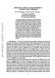
Introduction Consider a water well that taps into an underground aquifer and allows groundwater to be pumped out and supplied to a small village. In order to assess the rate at which the groundwater can be extracted, the hydraulic conductivity of the aquifer (among other parameters) is required. This is a measure of how fast groundwater can move through the pore spaces in the aquifer and typically varies spatially. Without access to conduct material experiments on the aquifer material, how can one determine its hydraulic conductivity? By solving an inverse problem. Inverse problems allow us to gauge parameters we cannot directly observe, provided there exists a forward model which maps the parameters to some observable output. The hydraulic conductivity field of an aquifer can be estimated by inverting hydraulic pressure readings taken from boreholes. In this case, the forward model is the steady flow in porous media partial differential equation (PDE) and the hydraulic pressure readings are the measurable data (refer Figure 1.1).

Figure 1.1: Inversion problem in terms of hydraulic conductivity To solve this inverse problem, one might first try a linear regression technique to find hydraulic conductivity or parameter values which fit the measured data in the least squares minimisation sense, such that residual values between the measured data and model predicted output are sufficiently small. Unfortunately, as it is commonly the case in nature, it is unlikely that a single, unique parameter will satisfy the minimisation problem. When inverting hydraulic pressure data, it is common for the measured data (discrete pressure readings from boreholes) to outnumber the desired number of 1

2

CHAPTER 1. INTRODUCTION

unknowns (spatially distributed parameter values) and the problem is therefore underdetermined [1]. To make the problem unique, it is common to add a regularisation term to the least squares minimisation formulation. This has the benefit of finding a unique hydraulic conductivity field K that minimises the regularised formulation but gives no indication of its correctness. Conversely, statistical inversion returns a probability density function over the parameter space providing a means to quantify the uncertainty of the recovered K. However, given the hydraulic conductivity field is a spatially distributed parameter, it is a tremendous challenge for the statistical inversion sampling algorithm to explore the high dimensional parameter space. Given no prior knowledge, the region of study is generally parameterised to align with the number of elements used in the discretisation process which, for a three-dimensional problem, can easily mean a parameter space dimensionality in the order of a million. The statistical inversion process attempts to recover a probability density function over the entire parameter space, for which every sampled value requires solving the forward problem. The challenge faced by the sampling method of exploring the high dimensional parameter space in finite time soon becomes impractical if we desire a parameter field that is at least somewhat informative. Therefore, in order to recover the hydraulic conductivity field complete with uncertainty quantification, it is necessary to implement parameter space reduction techniques. This is the focus of the present works. The objective of this thesis is to improve on current statistical inversion methods which leverage off parameter space reduction techniques.

1.1

Inverse Problems

Inverse problems, as the name suggests, are the inverse of forward models. Forward models are physical models that make predictions on the results of well-described physical systems, they allow us to predict the outcome given some known parameters. For example, given the hydraulic conductivity field discussed above, we could uniquely predict the hydraulic pressure distribution over the domain. The inverse problem for this example would be to predict the parameter, or hydraulic conductivity field, based on hydraulic pressure readings measured from boreholes. There are numerous ways to solve inverse problems but the most popular methods are regularisation or statistical inference, the former being the focus of this Section. Regularisation is a process of introducing additional information to prevent over- or under-fitting of mathematical models [2]. The technique was first developed in 1977 and is commonly referred to as Tikhonov regularisation inversion or classical regularisation inversion. An inverse problem is generally formulated as an optimisation problem where an objective function is minimised subject to the constraints of the forward model [3]. Consider the linear system, Ap = yd where A represents the discretised forward model that, when applied to parameter p, produces a model

1.2. STATISTICAL INVERSE PROBLEMS

3

predicted output that is directly comparable to measured data yd . In nature, it is uncommon for a single, unique p to satisfy this linear system. What we typically find is that no p satisfies the linear system, there is likely no p that satisfies the linear system, or infinite p’s that do. Problems lacking existence and/or uniqueness in this manner are defined as ill-posed, where properties for well-posed problems are 1) a p exists; 2) the p is unique; and 3) the p reacts predictably to changes in the measurement data yd [4]. Ill-posed problems often lead to under-determined systems which generally can’t be solved via traditional techniques such as least squares minimisation, that is, to find a unique p that minimises kAp − yd k2 . It is therefore common to apply regularisation to hydraulic conductivity inverse problems [1]. Tikhonov regularisation forces the problem towards parameters with a specific additional feature, for instance with the smallest gradient. Instead of attempting to solve the original problem exactly, Tikhonov regularisation modifies the problem as something that is close to the original by adding a penalty term to the cost function such that the new problem is solvable, unique, and reacts to changes in measurement data continuously or predictably. Tikhonov regularisation produces a new but similar problem where only a single hydraulic conductivity field K = p will reproduce the measurement data yd , and that the hydraulic conductivity field reacts continuously to changes in the measurement data. In equation form, this is equivalent to minimising the cost function kAp − yd k2 + µkpk2 , where µ is the Tikhonov regularisation parameter. Calculating the optimal Tikhonov regularisation parameter is a difficult endeavour but there are numerous publications which provide methods to do this [5–8].

1.2

Statistical Inverse Problems

Tikhonov Regularisation is deterministic in the sense that a unique parameter p is the solution to the inverse problem. It therefore restricts the solution to a single estimate of the parameter. This is not too dissimilar from Classical or Frequentist methods for statistical inversion such as the Geostatistical Approach and the Maximum a posteriori (MAP) in the sense that they are deterministic [3]. Inverse solutions are found by solving an optimisation problem [9]. The MAP estimate finds the parameter which has the greatest likelihood of reproducing the measured data, still capable of incorporating prior knowledge but returns only a point estimate of the mode of the posterior distribution. Parameter estimation via the Geostatistical Approach is carried out in two stages, the first of which being structural analysis where an empirical model is derived which adequately characterises the parameter field in a sufficiently low dimensional parameter space. The second stage, similar to that of MAP, is to solve the optimisation problem which fits the model predicted output to the measured data by adjusting the characterised parameter field. Uncertainty quantification with the Classical approach is achieved through analysis of the probability of events in the sample space associated with data. For the MAP recovered parameter field, the Classical approach allows us to quantify how certain we are that a particular hydraulic pressure field will eventuate, however, we are uncertain as to how likely it is

4


that a particular parameter field will reproduce data-consistent pressure values, in other words, we are still uncertain of the recovered MAP parameter fields ability to reproduce data-consistent hydraulic pressure value. As mentioned above, the Geostatistical approach provides best estimates as well as measures for uncertainty quantification but this can be a computationally expensive exercise as the Jacobian is required and it is an iterative process. The reality that the observable data is generally informative about low dimensional manifolds of parameter space can be exploited to reduce computational cost. The theory presented in [10] leverages of this notion to allow construction a low-rank approximation of the posterior probability density function covariance matrix, that is, the principal components of the covariance matrix are used allow its approximation in low-rank form. This facilitates a reduction in both the number of forward model evaluations and cost of matrix manipulation. Statistical Inversion in the Bayesian sense returns a probability density function over the parameter space describing the relative likelihood of the selected parameter being consistent with the measured data. The inverse problem is reformulated as a statistical inference problem by means of Bayesian statistics [11]. Rather than solely recasting the model predicted output as a random variable, as is the case with Classical methods, the Bayesian approach allows all unknowns to be modelled as random variables, for which posterior probability density functions are recovered via sampling methods [12]. Modelling all quantities as random variables is representative of level of uncertainty common to ill-posed problems. It is a technique that allows us to infer possible solutions based on the success or failure of previous attempts. Previous attempts are ranked and the corresponding level of uncertainty is quantified. The result is a probability density function over a set of parameter estimates from which the expected values, and other desired moments, can be obtained. In terms of the linear system presented above, the theory requires that both the parameter p and model predicted output y(p) = Ap are treated as random variables where the probability density of the parameter conditioned on the model predicted output, referred to as the posterior distribution, is what we seek to recover via statistical inversion. The Bayesian approach naturally incorporates prior information about the solution but most importantly, it provides the likelihood of parameter values being consistent with the measured data and is therefore more suitable than Classical or Frequentist methods for ill-posed problems with expected measurement error. It is the focus of the current works. Spatially distributed parameters present a significant challenge to recover via statistical inversion due to the high dimensionality of the parameter space. Methods exist which split the domain into a number of ”pixels”. Rosas, M. et al. carried out a 2-D pixel-based MCMC inversion geophysical data inversion study [13]. Each pixel in the domain is characterised by a model parameter which is projected through the a forward model, combined with a nominal noise term, and then compared with the measurement data. Bayes theorem is invoked to derive a relationship between the posterior distribution of the model parameter conditioned on the data, a likelihood function, and prior information of

5

1.2. STATISTICAL INVERSE PROBLEMS

the data and model parameters. The likelihood function is constrained by the vertical soil resistivity profile. Using MCMC methods, the authors recover marginal posterior probability density functions of the three vertical resistivity profiles delineated by the letters V 1, V 2 and V 3 shown on the surface of the 2-D domain (refer Figure 1.2 (a) and (c)).

(a) Synthetic resistivity field

(b) MCMC recovered resistivity field

(c) MCMC recovered recovered marginal posterior probability density functions of three vertical resistivity profiles

Figure 1.2: Pixel-based MCMC inversion of geophysical data Similarly, classifying the domain into discrete ”geological units”, allows material properties within each unit to be recovered by statistical inversion. Jardani, A. et al. apply this technique to 2-D seismic and seismoloeletric signals [14]. The goal is to recover posterior distributions over a deep reservoirs’ hydraulic conductivity and other properties. The authors split the domain into three geological units based on prior knowledge. These include two sedimentary layers (L1 and L2) and one reservoir (R) (refer Figure 1.3). IR1-IR5 correspond to the arrival of the P-waves at each interface. P-waves are elastic constants characteristic of material property types. The prior knowledge in this case is the presence of an oil reservoir, its approximate location and extent, as well as an approximate depth of the boundary between the two sedimentary layers. The corresponding Bayesian formulation recasts the various material properties as random variables, of which the posterior distributions are recovered via MCMC sampling. The forward model in this case is the wave equation which is incorporated via the likelihood function. Alternatively, the sampling process can be accelerated by implementing active subspace techniques [15]. This researches leverages of the virtue that inverse problems are typically ill-posed where

6


Figure 1.3: Geological unit-based MCMC inversion of geophysical data the data does not inform all parameters. They seek to hone in on the parameters which are informed by the data while glossing over others. Provided an active subspace exists for the problem, the MCMC algorithm can exploit its low-dimensional structure and sample more efficiently than attempting to explore the entire high-dimensional complete parameter space. This technique was adapted from the subspace-based dimension reduction method presented in [16] which identifies a likelihood-informed subspace by characterising the relative influences of the prior and the likelihood over the support of the posterior distribution. To simultaneously combat the two biggest challenges of MCMC sampling methods used to solve statistical inverse problems governed by PDE’s - that is, high-dimensional parameter space, and costly forward model evaluations - a so called Stochastic Newton method [17] can be implemented. This method approximates the target probability density function with a (local) Hessian-informed Gaussian process which is used as the proposal density for the MCMC process. The focus of the current works, however, are implementing parameter space reduction techniques to approximate the parameter field by an informative but low dimensional basis [18]. In a similar manner, the solution to the forward model can be approximated in a low dimensional space to expedite forward model evaluations and therefore posterior sampling [18]. This parameter space reduction technique was also successfully implemented in the context of Tsunami modelling [19]. The authors present a model that reconstructs the source of a tsunami from data recorded by surrounding observation systems. They recover the coefficients for a series

1.3. GEOPHYSICAL INVERSION

7

of Gaussian basis functions centred at uniformly spaced grid points representing initial sea surface displacements.

1.3

Geophysical Inversion

Observable or measurable geophysical data which can be inverted include electrical potential to recover electrical resistivity [20]; hydraulic pressure to recover hydraulic conductivity [21]; tsunami wave propagation to recover initial sea surface displacement [19]; seismic waveform data to recover density [22]; surface gravity data to recover distribution of density contrast [23]; and surface magnetic data to recover susceptibility profiles [24] to list but a few. The current works, however, gives most attention to inverting hydraulic pressure and electrical potential data. So far we have discussed the form of least squares minimisation for linear problems or linear regression and Tikhonov Regularisation inversion as methods of recovering spatially distributed parameters from a measured data but we have yet to discuss the available methods for solving the optimisation problem. For this we can use iterative methods such as Conjugate Gradient [25, 26] and Kaczmarz’s algorithm [27]; spectral methods by Fourier transforms [28]; Gauss-Newton method for non-linear least-squares problems [29]; Occam’s Inversion [30] among others not discussed here.

1.4

Motivation

Scientists and engineers must have a level of confidence in their computed inverse solutions. This is challenging if their solutions are obtained via deterministic inversion. Uncertainty arises from a number of traits intrinsic to deterministic inverse problems as introduced in the preceding sections. The problem may lack a solution entirely if the forward model is only approximate due to noise or discretisation errors; the solution may lack uniqueness where more than one solution fits the data exactly; or if computation of the solution is unstable and acts unpredictably given small changes in measurement data [3]. We know the introduction of regularisation modifies the problem so a unique solution can be found but we are uncertain of the ramifications of this modification. Finally, all measurement data contain errors. Consider the potential error of an unstable inverse solution subject to even a modest amount of measurement error! It cannot safely be ignored. Statistical inversion allows us to implement expected bounds on measurement error a-priori in such forms as mean values and standard deviations, and will generate a-posterior distribution from which the sampled variance of the model predicted output can be extracted. It allows us to estimate the actual error in the model and data by modelling expected errors into the analysis [31]. The parameter posterior distribution provides probabilities for measurement-consistent parameter values. Therefore statistical inversion allows scientists and engineers to make informed decisions from their inverse solutions.

8


Statistical inverse problems which recover spatially distributed parameters are a difficult and time consuming endeavours. To obtain good posterior estimates, it is important to ensure the high dimensional parameter space has been sufficiently explored during the sampling process. To serve as a rough indication of the required computational effort of a statistical inverse problem for given a parameter space dimensionality, let us consider a study conducted on the convergence time, among other properties, of various sampling algorithms [32]. For the widely known Metropolis-Hastings sampling algorithm [33, 34], it is shown that the required number of likelihood evaluations Nlike to achieve convergence scales linearly with dimension D, that is, Nlike = 330D. When each likelihood evaluation requires solving a PDE one or more times, recovering a spatially distributed parameter field, which may have a dimensionality in the millions, quickly becomes intractable. There are more efficient sampling algorithms available today but these often scale exponentially with dimension due to the dilution of volume distribution with increasing dimension [35]. These concepts will be developed further in Chapter 4. The parameter space reduction techniques presented by Lieberman et al. [18] require that only a dozen basis function coefficients are recovered by statistical inversion, a significant reduction compared to previous methods. The intent of the current works is to improve on this method by implementing in continuous function space, as opposed to the discrete Euclidean space. It is the hope that the continuous setting will facilitate mesh independence so unstructured mesh can be used, as well as improving optimisation and orthonormalisation efficiency. Applying the method to data analogous to that of electrical resistivity tomography (ERT) is a compelling motivation also and will therefore be included in the current works.

1.5

Chapter Outline

This thesis is divided into seven chapters, including this Introduction and a Discussion and Conclusion chapter. There is also a set of appendices with peripheral information. In chapter two we discuss the various methods for model and parameter space reduction before introducing the forward problem. We present the adopted Greedy Sampling algorithm and derive the associated optimisation problem. Chapter three is where we introduce the optimisation algorithm used in each Greedy cycle and explain the procedure for constructing the reduced bases. In chapter four we present various Markov chain Monte Carlo sampling methods and then formulate the Bayesian Inference model used to find the solution to the inverse problem. Chapter five provides details on the implementation including utilised software modules, model checking functions, and some additional fundamental theory for the current works. In chapter six we present results from numerical experiments on groundwater flow and electrical resistivity type problems. Chapter seven is where we summarise important results and conclude the thesis the main findings, any limitations and proposed future work.

Chapter 2

Model and Parameter Space Reduction

In this chapter we discuss the different model and parameter space reduction techniques which have already been successfully implemented. We also define, in greater detail, the different forward models adopted for the current works. Some formulae are introduced.

2.1

Introduction

Model reduction techniques allow us to produce a low-order approximation of a model which is still adequately representative of the original model but which possesses computational efficiency. This is achieved by reducing the models complexity and/or dimension [36]. In the statistical inverse setting, model reduction facilitates faster forward model solves and thus faster sampling from the posterior distribution. When the intent is to recover a spatially distributed parameter, however, the sampling algorithm will still struggle to adequately explore the high dimensional parameter space. In this case, parameter space reduction techniques can be implemented, which, similar to model reduction techniques, allows the parameter to be approximated by a low dimensional proxy. This is an effective technique since the observed data is not informed by the entire parameter space for ill-posed problems [37]. Thus, confining the parameter space to that which is informative often has little effect on the accuracy of the inverse solution.

2.2

Model and Parameter Space Reduction

There are a number of existing model reduction methods which are compatible with non-parametric models, that is, models that do not depend on parameters. These include Proper Orthogonal Decomposition (POD), applied to an optimal control problem for a linear heat equation for example [38] or Krylov subspace techniques, which are popular for reduced order modelling of large-scale dynamical systems [39]. Alternatively, Balanced Truncation is a suitable model reduction technique for problems like the semi-discretised Stokes equation [40]. 9

10

CHAPTER 2. MODEL AND PARAMETER SPACE REDUCTION

Methods that are compatible with parametric models such as hydraulic conductivity problems are the so-called Reduced-Basis or Projection-Based methods. In these methods, the reduced basis is a set of state functions computed by solving the full model for a selected set of parameter values [41]. As is common with parameterised models, the parameter space is generally much larger than that of the data and the problems are therefore highly underdetermined and very sensitive to small changes in parameter values. There are a number of methods available to construct these bases such as Principal Component Analysis, Singular Value Decomposition (SVD), Discrete Cosine Transform and the Discrete Wavelet Transform [37]. The process of selecting the next parameter from which the next state function can be computed is controlled by a Greedy Sampling algorithm. This algorithm was introduced to overcome the challenge of sampling from high-dimensional parameter space [42, 43]. The intent of each Greedy Sampling iteration is to identify a basis function for which the estimated defect between the full and reduced model predicted output y(p) − yr (pr ) is maximum. Each Greedy Sampling iteration is an optimisation problem that returns a basis function in the parameter space.

In the current works, we adopt a Proper Orthogonal Decomposition variant with a spectral component generalised for parametric model compatibility to simultaneously construct state u and parameter p bases via Greedy Sampling. By assuming a quadratic form for the forward problem, the defect between the full and reduced model predicted output can be approximated by an iterative approach to its spectral decomposition similar to that presented in [44]. This defect is the primary component of the cost function for the optimisation problem to be solved for each Greedy Sampling iteration and each new basis function.

2.3

Forward Model

A forward model is a well understood physical system that can be modelled mathematically. The mathematical model that describes the physical system can take many forms, for example, the motion of a simple pendulum is governed by an Ordinary Differential Equation (ODE) that predicts the angle of the pendulum at a given time; the mass of an unknown composite is subject to the integral equation of its density distribution constrained by its volume; and the optimal strategy for minimising losses in rock-paper-scissors using game theory can only be modelled as a numerical algorithm as no analytical model exists. The groundwater problem presented in the Chapter 1, however, is governed by a partial differential equation (PDE) which is defined below. Each of these forward models could be formulated as inverse problems if desired but the focus of this thesis is PDE constrained inverse problems.

The forward model of the groundwater problem is governed by the steady flow in porous media

11

2.3. FORWARD MODEL

PDE. This PDE, along with appropriate boundary conditions is defined below: −∇ · (K∇u) = f in Ω,

(2.1)

K∇u ·~n = 0 on ΓN , u = 0 on ΓD , where Ω represents the domain, ΓN the Neumann boundary, ΓD the Dirichlet boundary, K(x) the hydraulic conductivity field, f (x) the hydraulic source or sink function, and u(x) both the hydraulic pressure field and solution to the PDE. Symbols ∇ and ∇· refer to the gradient and divergence operators respectively. The forward model is not yet complete, however, some post-processing of the PDE’s solution is require as we are only interested in values at sensor locations. Additionally, the hydraulic conductivity field requires parameterising to ensure only positive values are subbed into the PDE. The forward model is therefore a function that maps the parameter field p(x) ∈ P to model predicted output y ∈ Y, that is, M : P → Y. This mapping allows the model predicted output to be directly compared to the measurement data yd as required for inverse problems. The parameterisation of the hydraulic conductivity field is chosen as follows: K(x) = K0 e p(x) ,

(2.2)

where K0 is a known or assumed a-priori reference hydraulic conductivity value typically chosen as a constant. The majority of the derivations to follow are carried out in continuous function space, however, for illustrative purposes, is it useful to develop the discretised forward model: A(p)u = f, y = Cu, y(p) = C[A(p)]−1 f,

(2.3)

where A ∈ RN×N and represents the discrete forward operator. The vector p ∈ RN contains the discrete parameter values. The vector u ∈ RN is the solution to the PDE. The vector f ∈ RN represents the hydraulic source or sink values discretised over the domain. Vector y(p) ∈ RN0 is the model predicted output. Finally, C ∈ RN0 ×N is the observation operator which converts u to a variable comparable to the measurement data yd . The solution u is found via either Finite Element Methods (FEM) [45] or Finite Difference Methods (FDM) [46] (refer § 5.3.2). Notice the forward operator A is a function of parameter p and the forward model is therefore nonlinear in the parameter p. It should be noted that the groundwater flow problem presented above is a simplification of Hydraulic Tomography inversion [47] which is more commonly used in the geophysical inversion field. With Hydraulic Tomography, a series of pump tests are carried out and therefore more data is produced, allowing a more accurate inverse solution to be obtained. Similarly, Electrical Resistivity Tomography

12


(ERT) is a technique which gathers data from a series of injection tests which can be inverted to recover the subterranean conductivity/resistivity field. Conversely, with ERT, injections are electrical current and the measurable data are electric potential. The amount of data obtainable with ERT is comparatively large [48]. In the current works, we focus on two geophysical inversion cases 1) the groundwater flow problem already introduced; and 2) an electrical conductivity problem analogous to ERT. The groundwater flow problem is modelled in 2-D with only a single experiment and sensors dispersed uniformly over the domain. The electrical conductivity problem is also modelled in 2-D, however, there is a series of tests conducted and the sensors are located on only one boundary - the surface. The PDE is the same in both cases.

2.4

Greedy Sampling

The state u and parameter p bases are constructed ”offline” in the sense that they are produced prior to the MCMC sampling commences. They are constructed during the Greedy Sampling process. The information required to construct the bases are: • forward model; • domain and boundary conditions; • location, type and magnitude of sources; • location of sensors; and • reference conductivity for obtaining parameterisation. The two bases do not assume to know anything about the parameter field which we attempt to recover (aside from the expected smoothness) therefore their construction need only be done once. It is worth constructing a set of informative basis functions to approximate both the parameter and state even at the expense of additional computational work. The ensuing ”online” phase, that is, the MCMC sampling process, will be more efficient and recover a more accurate inverse solution if this is the case. The Greedy Sampling process adopted in the current works boils down to the solutions of a series of optimisation problems. Each optimisation problem finds a parameter field that maximises the defect between the full and reduced model predicted output y(p) − yr (pr ). Maximising the defect allows us to capture the maximum amount of information available in the current optimisation problem. The resulting parameter field pk and corresponding state function u are orthogonalised via Gram-Schmidt with their existing basis function counterparts and normalised (refer § 2.4.2) before being stored in their respective bases.

13

2.4. GREEDY SAMPLING

2.4.1

Greedy Optimisation Problem

As mentioned above, for each Greedy Sampling iteration we want to find the parameter p that maximises the defect between the full and reduced model predicted output y(p) − yr (pr ). Therefore, for the kth Greedy Sampling iteration we start with the squared norm of the defect Rˆ k as 1 Rˆ k (p) = ky(p) − yr (pr )k2L2 (Ω) 2

(2.4)

where k · kL2 (Ω) is the selected L2 norm over domain Ω: kak2L2 (Ω)

Z

=

|a|2 dx.

Ω

It is obvious that attempting to maximise Equation (2.4) over p will result in infinite defect. We therefore scale Rˆ k by the norm of the parameter field r r 2 1 ky(p) − y (p )kL2 (Ω) Rk (p) = 2 [p, p]

(2.5)

where [p, p] represents an appropriately chosen norm. In the continuous setting, the post-processing of the PDE solution is carried out via a weighting function w(x) (refer Figure 6.5 for a graphical representation of this) which is non-zero at locations where data is available, therefore y(p) = w u(p). The reduced state function ur , from yr (pr ) = w ur (pr ), approximates the full state function by a truncated linear combination of basis functions: ur (x) = ∑ αl vl (x)

(2.6)

l

for l = 0, ..., k. There is always k + 1 state basis functions since v0 is the orthonormalised state function u(0). The basis function coefficient is delineated by αl and vl corresponds to the state basis functions. Similarly, the reduced parameter field pr approximates the full parameter field by a truncated linear combination of basis functions: pr (x) = ∑ β j q j (x)

(2.7)

j

for j = 1, ..., k meaning there is always one less parameter basis function than state state basis function. The validity of this constraint is discussed further in 6.2.8. The parameter basis function coefficients are delineated by β j and q j corresponds to the parameter basis functions. To ascertain a suitable norm for the denominator of the cost function (2.5) we apply a spectral decomposition. Making the assumption that y(p) − yr (pr ) = 0 for p = pr allows us to impose a linear approximation on the model defect and subsequently adopt a quadratic form for the objective function. The validity of this assumption is tested in § 6.2.9. Returning to the discrete setting for a moment to illustrate the effect of the linear approximation we can write the following: y(p) − yr (pr ) = Dp

(2.8)

14


for linear operator D. Equation (2.5) can then be written in quadratic form: Rk (p) =

1 pT DT Dp . 2 pT Sp

(2.9)

for parameter norm kpk2S = pT ST p and linear operator S. Now let λ j and q j represent the eigenvalues and eigenvectors of the generalised eigenproblem: DT Dq j = λ j Sq j

(2.10)

Which, for symmetric-positive-definite (SPD) S, has real non-negative eigenvalues λ j ≥ 0 and a basis of orthogonal eigenvectors qi Sq j = δi j (refer to § A.2 for Kronecker Delta δi j theory). In the discrete setting, the parameter field is approximated by a linear combination of orthogonal basis vectors or eigenvectors in the linearised case, therefore: p = ∑ β jq j j

thus Equation 2.9 reduces to 2 1 ∑ j λ jβ j Rk (p) = 2 ∑ j β j2

(2.11)

which demonstrates that the largest eigenvalue is λ1 which corresponds to basis vector q1 . Notice that it does not matter what parameter norm is adopted, as it is SPD. Thus, we now define a suitable norm which satisfies the SPD requirements in the continuous setting, that is, the scaled H 1 norm as follows and henceforth represented by square brackets: Z

[p, q] =

(µ0 · p · q + µ1 ∇p · ∇q) dx

(2.12)

Ω

with appropriately chosen non-negative trade-off factors µ0 , µ1 . Similar to the case for the orthogonal eigenvectors (2.10), the following relationship exists between the orthonormal parameter basis functions: [qi , q j ] = δi j .

(2.13)

Additionally, as we will see in § 3.3.1 each iterate (parameter) returned by the optimisation algorithm is orthogonal to the Q-basis and therefore: [p, q j ] = 0 for j < k

(2.14)

As we will see in § 2.4.2, Condition (2.14) allows us to write β j = [p, q j ], and therefore rewrite Equation (2.11) in continuous form and in terms of orthogonal p 1 ∑ j≤k λ j [p, q j ]2 . Rk (p) = 2 ∑ j≤k [p, q j ]2

(2.15)

We saw above that the the spectral decomposition of the discrete case resulted in the largest eigenvalue being targeted first due to condition (2.13). A nice result of condition (2.14) is that the optimisation problem will always pick the next smallest eigenvalue.

15

2.5. REDUCED MODEL

2.4.2

Orthonormalisation

Each iteration of the Greedy Sampling algorithm requires solving the optimisation problem derived in the previous section. Specifically, we are required to find the pk+1 that minimises the objective function (2.5). This pk+1 is then used as the input parameter to solve the forward model PDE (2.1) subject to parameterisation (2.2). The resulting PDE solution uk+1 , along with the parameter pk+1 , then require orthonormalisation and storage. The Gram-Schmidt procedure is to take the next orthogonal parameter basis function q˜k+1 equal to the next parameter field pk+1 less some linear combination of the previous orthonormal basis functions q j ∈ Q for j = 1, ..., k [49]. The contribution of each existing q j ∈ Q is found via the following projection: projq j (pk+1 ) = [q j , pk+1 ] q j with scaled H 1 norm [q j , pk+1 ] from (2.12). Therefore, adding a new orthogonal p is achieved via the following: k

q˜k+1 = pk+1 − ∑ projq j (pk+1 ), j=1

and normalisation is carried out using scaled H 1 norm: qk+1 =

q˜k+1 . [q˜k+1 , q˜k+1 ]

The new orthonormalised parameter field qk+1 is appended to the parameter basis Qk . A similar process is carried out for the next state function uk+1 to give the orthonormal state basis function vk+1 which is then appended to the state basis V with the exception of the norm used. For the state basis we use inner product h·i k

v˜k+1 = uk+1 − ∑ hvi , uk+1 ivi , i=0

v˜k+1 vk+1 = hv˜k+1 , v˜k+1 i With these bases we can represent the parameter field p and state u with reduced approximations pr and ur by projecting p onto Q and u onto Vk+1 respectively as follows: pr ∈ span{q1 , ..., qk }, ur ∈ span{v0 , ..., vk }, as seen in Equations (2.6) and (2.7).

2.5

Reduced Model

Recalling the forward model M : P → Y from § 2.3, we find the solution of the PDE, u ∈ U and parameter field p ∈ P. We now nominate subspaces where we expect to find the reduced state ur ∈ Ur ⊂ U

16


and reduced parameter field pr ∈ Pr ⊂ P. We enforce the criteria to ensure the subsets Ur and Pr can be considered subspaces, that is, they contain the zero function; are closed under scalar multiplication; and are closed under addition. As seen in the previous section, the reduced state ur is obtained by projecting state function u onto state basis V . This approach is commonly known as the Galerkin projection [36]. We expect u ∈ / Ur and p ∈ / Pr , therefore the Galerkin projections on subspaces Ur and Pr , are our best approximations of the parameter and state. From the Greedy Sampling algorithm, we have our state basis V and parameter basis Q, and can therefore approximate the subspace by some linear combination of the basis functions Ur = span(V ) and Pr = span(Q). The orthonormal bases V and Q are minimum sets of linearly independent basis functions that span the subspace Ur and Pr respectively. We assume u ∈ U can be adequately approximated by ur ∈ Ur , and likewise that p ∈ P can be adequately approximated by pr ∈ Pr . We have seen that ur ∈ span{v0 , ..., vk } and pr ∈ span{q1 , ..., qk )}, but we can also approximate the source function f in f r ∈ span{v0 , ..., vk } as it also exists in the state subspace. The Galerkin projection in the continuous setting amounts to the following for Ur : k

ur = projV (u) =

∑ < vl , u > vl l=0 k

= ∑ αi vi i=0

for (αi ) = α ∈ Rk+1 and inner product: Z

< a, b > =

a(x) b(x) dx. Ω

Similarly for the source function, f : k

f r = projV ( f ) = ∑ < vi , f > vi i=0 k

= ∑ γi vi i=0

for (γi ) = γ ∈ Rk+1 . The parameter space projection is carried out as follows: k

pr = projQ (p) =

∑ [q j , p] q j

j=1 k

=

∑ β jq j

j=1

for (β j ) = β ∈ Rk . The reduced form of the steady flow in porous media PDE becomes: −∇ · (K(pr ) · ∇ur ) = f

17

2.5. REDUCED MODEL

with weak form: Z

K(pr )∇ψ r · ∇ur dx =

Ω

Z

ψ r f dx for all ψ r

Ω

for ψ r ∈ U also. We can expand this using the above projections for ur and ψ r : k

k

K (p )∇v j · ∇vi dx α j =

Z

∑ ∑ θj

j=0 i=0

r

r

Ω

k

∑ θj

j=1

Z

v j f dx

Ω

for all (θ j ) = θ ∈ Rk+1 . We can now define the reduced stiffness matrix Ar ∈ R(k+1)×(k+1) in component form as follows: Arij

Z

=

K(pr )∇v j · ∇vi dx for i, j = 0, . . . , k

(2.16)

Ω

which naturally leads to the matrix-vector relationship: Ar α = γ and is easily solved for (α j ) = α ∈ Rk+1 . The reduced state ur is then calculated via (2.6).

(2.17)

Chapter 3

Optimisation and Basis Construction

This chapter provides the optimisation algorithm adopted for solving the Greedy Sampling minimisation problem. This algorithm requires the analytical gradient of the cost function (2.5) and an approximation to the Hessian operator of the cost function (2.5).

The particular implementation of the optimisation problem presented in the current works is consistent with that previously published by Codd, A et al. [50]. Optimisation is a peripheral but necessary attribute of the current works and therefore, aside from some minor differences, Sections 3.3.1 and 3.3.2 are largely extracted from the aforementioned publication.

3.1

Introduction

In this chapter we develop the optimisation algorithm adopted for the Greedy Sampling process. For this we use the quasi-Newton algorithm named for its discoverers, Broyden-Fletcher-Goldfarb-Shanno (BFGS) [51]. The BFGS method has the benefit of being self-preconditioning and avoids the need for constructing the dense Hessian. The optimisation is performed in an appropriate function space [50].

The Greedy Sampling Optimisation problem is comparable to a deterministic inverse problem. At each Greedy cycle we find a single estimate of the parameter field pk+1 that maximises the cost function (2.5). In the implementation we minimise −Rk . We assume the defect y(p) − yr (pr ) = Dp is linear in p for some linear operator D but expect that is in fact non-linear. The resulting quadratic form of the cost function facilitates a spectral decomposition where the final eigenvalue correspond to the expected maximum residual at each Greedy Sampling iteration. The deterministic inverse problem is to ”recover” the parameter field that minimises the residual value −Rk for each iteration. However, instead of comparing the model predicted output y(p) to some observable data yd , we compare full y(p) with the reduced model predicted yr (pr ). 19

20

CHAPTER 3. OPTIMISATION AND BASIS CONSTRUCTION

3.2

Optimisation Problem

Each Cycle of the Greedy Sampling optimisation problem finds a local minima, the point at which the cost function is smaller than all other surrounding points, and is therefore classifiable as a local optimisation problem. This is common for non-linear optimisation problems. Evaluations of the cost function are restricted by the state space U and reduced state space Ur , that is, the obtainable solutions from the forward model and the reduced model, therefore the problem is constrained. As mentioned in the introduction, we adopt the limited-memory BFGS (L-BFGS) algorithm to minimise our cost function (2.5). This version of the BFGS algorithm stores gradient differences and search directions for a fixed number of previous iterations, denoted a. For the cost function R and parameter p, the convex quadratic model at the ith iteration of the optimisation algorithm is obtained by truncating the Taylor expansion after the second order derivative as follows: 1 (3.1) mk (si ) = Rk (pi ) + h∇Rk (pi ), si i + h∇∇Rk (pi )si , si i, 2 for an appropriate inner product h.i, property function mk , cost function gradient ∇Rk (pi ), Hessian operator ∇∇Rk (pi ) and search direction si which is also the increment in the Taylor series. The search direction allows us to calculate the next iterate pi+1 of the optimisation problem. Solving the quadratic model (3.1) allows us to calculate the the search direction si si = −[∇∇Rk (pi )]−1 ∇Rk (pi ).

(3.2)

As is commonly the case with Newton-type methods for optimisation problems, it is expensive to construct the Hessian operator exactly. Fortunately, the robustness of the BFGS algorithm means it can accept an approximation to the Hessian operator. In the following sections we derive the analytical gradient ∇Rk and an approximation to the Hessian operator ∇∇Rk .

3.2.1

Cost Function Gradient

As seen in (3.2), we require the analytical gradient of the cost function ∇Rk (pi ). To derive this we adopt a technique implemented by Codd, A. et al. [50] and extend to cater for the reduced model component (2.5). The method requires solving an adjoint PDE similar to (2.1) but instead of the right-hand-side of the PDE being the source function, it is equal to the current defect between the observed data and the mode predicted output. The implementation in the current works of course differs in that we have no data term. We start with the vanishing Gateaux derivative formulated in the following manner, ∂ Rk (p + ε · δ p) h∇Rk (p), δ pi = = 0, ∂ε ε=0

(3.3)

for ε small and any incremental change in parameter value δ p. Using this formulation and the quotient rule for differentiation, we obtain the desired form the the cost function gradient: h∇Rk (p), δ pi =

1 Rk (p) h∇Rˆ k (p), δ pi − 2 [p, δ p] [p, p] [p, p]2

21

3.2. OPTIMISATION PROBLEM

for a given direction δ p. Recall Rˆ k is the norm of the model defect 1 Rˆ k = ky(p) − yr (pr )k2L2 (Ω) 2Z 2 1 = w2 u(p) − ur (pr ) dx 2 Ω for weighting function w introduced in § 2.4.1. We can now define the gradient of the model defect norm h∇Rˆ k (p), δ pi =

Z

w2 (u(p) − ur (pr )) δ u dx −

Ω

Z

w2 (u(p) − ur (pr )) δ ur dx

(3.4)

Ω

where δ u and δ ur are increments in the full state u and reduced state ur due to increment δ p. The gradients of these are derived by solving a number of adjoint problems. To derive the first term, that is, the defect incremented by the full state, we start with the original PDE (2.1) −∇ · (K∇u) = f in Ω, and apply increment ∇ · (K(p + εδ p)∇(u + εδ u)) = f .

(3.5)

before making the first order approximation K(p + ε δ p) ≈ K(p) + ε K 0 δ p where K 0 represents the derivative of the conductivity field with respect to the parameter p, −∇ · K(p) + εK 0 (p)δ p) ∇(u + εδ u) = f . Expanding, then simplifying by ignoring higher order terms ε 2 given ε 2 → 0 faster than ε → 0, and using the original PDE to cancel zero order terms, the weak form of the incremented PDE can be written as Z

K∇ψ · ∇δ u dx = −

Z

Ω

K 0 δ p∇ψ · ∇u dx for all ψ.

(3.6)

Ω

Now we nominate an adjoint PDE such that the right hand side of the original PDE is equal to the model defect with squared weighting function Z

K∇u∗ · ∇ψ dx =

Ω

Z

w2 (u − ur ) ψ dx for all ψ.

Ω

for adjoint solution u∗ . By setting ψ = δ u, we get the following Z

∗

K∇u · ∇δ u dx =

Ω

Z

w2 (u − ur ) δ u dx.

Ω

which can be combined with the incremented forward PDE (3.6) after setting ψ = u∗ as follows Z

2

r

w (u − u ) δ u dx = −

Ω

Z

K 0 δ p∇u∗ · ∇u dx.

Ω

Now we have a solvable equation for the first term in the defect gradient. Refer to § 5.3.1 for details on how we solve this adjoint PDE for u∗ .

22


The second term in the defect gradient, i.e. the defect incremented by the reduced state δ ur , is derived in a similar fashion. The governing PDE for the reduced model can be defined in its weak form as follows Z

r

r

Z

r

K(p ) ∇ψ · ∇u dx =

Ω

ψ r f dx for all ψ r ∈ span(V ).

Ω

We solve this for ur via the method presented in § 2.5 and then nominate the reduced adjoint PDE in weak form as the following Z

r∗

r

Z

r

K(p )∇u · ∇ψ dx =

Ω

w2 (u − ur ) ψ r dx for all ψ r ∈ span(V )

Ω

Setting ψ r = δ ur we make a connection to the gradient defect (3.4) Z

r∗

r

r

K(p )∇u · ∇δ u dx =

Z

Ω

w2 (u − ur ) δ ur dx for all δ ur ∈ span(V )

Ω r∗

which can be solve for u (refer § C.1 for methodology). Analogously to what was done for the full model, we formulate an incremented PDE for the reduced model in weak form and simplify, Z

r

r

r

K(p )∇ψ · ∇δ u dx = −

Z

Ω

K 0 (pr )δ pr ∇ψ r · ∇ur dx for all ψ r

Ω

where K 0 (pr ) is the derivative of the hydraulic conductivity field with respect to the reduced parameter ∗

pr . By setting ψ r = ur we get Z

r∗

r

Z

r

K(p )∇u · ∇δ u dx = −

Ω

∗

K 0 (pr )δ pr ∇ur · ∇ur dx for all δ ur ,

Z Ω

w2 (u − ur ) δ ur dx for all δ ur ,

= Ω

which provides a link to the second part of the model defect derivative (3.4), Z

w2 (u − ur ) δ ur dx = −

Z

Ω

∗

K 0 (pr )δ pr ∇ur · ∇ur dx for all δ ur .

(3.7)

Ω

We must now find a relationship between δ pr and δ p. We now from § 2.4.2 that pr is the projection of p onto Q = span{q1 , ..., qk } defined as [qr , pr ] = [q, p] for all qr ∈ Q

(3.8)

[qr , δ pr ] = [q, δ p] for all qr ∈ Q

(3.9)

which allows us to write:

Now we define the third adjoint problem pr∗ ∈ Q −

Z

K 0 (pr )qr ∇ur∗ · ∇ur dx = [qr , pr∗ ] for all qr ∈ Q,

Ω

which we can solve for pr∗ (refer to § C.2 for methodology). If one sets qr = δ pr , −

Z Ω

∗

K 0 (pr )δ pr ∇ur · ∇ur dx = [δ pr , pr∗ ] for all δ pr

23

3.3. BFGS ALGORITHM

Then using (3.9) gives −

Z

0

∗

K r δ pr ∇ur · ∇ur dx = [pr∗ , δ p] for all δ p.

Ω

which is the solution to the second part of the model defect gradient from (3.7). Bringing it all together, h∇Rˆ ( p), δ pi =

Z

2

r

r

w (u(p) − u (p )) δ u dx −

ΩZ

Z

w2 (u(p) − ur (pr )) δ ur dx

Ω 0

=−

∗

K δ p∇u · ∇u dx − µ0

Z

Ω

r∗

δ p p dx − µ1

Z

Ω

∗

∇δ p · ∇pr dx for all δ p

Ω

We now have all the components to formulate the gradient of the cost function. We first expand the cost function (2.5) r r 2 1 ky(p) − y (p )kL2 (Ω) R(p) = − 2 [p, p]2 2 R 1 Ω w u(p) − ur (pr ) dx R R =− 2 µ0 Ω |p|2 dx + µ1 Ω |∇p|2 dx

and find 0 δ p∇u∗ · ∇u dx + µ r∗ r∗ 0 Ω δ p p dx + µ1 Ω ∇δ p · ∇p dx R R h∇R(p), δ pi = µ0 Ω |p|2 dx + µ1 Ω |∇p|2 dx R 2 R R r r dx µ0 Ω p δ p dx + µ1 Ω ∇p · ∇δ p dx Ω w u(p) − u (p ) + R 2 R µ0 Ω |p|2 dx + µ1 Ω |∇p|2 dx

R

R

ΩK

R

It is convenient to rewrite the derivative in the following format: h∇R(p), δ pi =

Z

(X · ∇δ p + Z δ p) dx

Ω

so we can split the derivative into two component variables X and Z ∗ 2µ1 Rˆ µ1 ∇pr ∇p + 2 [p, p] [p, p] 2µ0 Rˆ µ0 r∗ K0 Z= p+ p + ∇u · ∇u∗ 2 [p, p] [p, p] [p, p]

X=

(3.10) (3.11)

Where, as mentioned above, Z

(µ0 p · p + µ1 ∇p · ∇p) dx,

[p, p] = Ω

1 Rˆ = 2

3.3

Z

w2 (u(p) − ur (pr ))2 dx

Ω

BFGS Algorithm

Now we have derived the analytical gradient for the cost function h∇R(p), δ pi, all we need is an approximation to the Hessian operator to calculate the search direction si and the subsequent update

24


for the iterate pi . In the current works, similar to that implemented by Codd, A. et al. [50], we use the Hessian operator of the scaled H 1 norm (2.12) Z

Z

∇[pi , pi ] = µ0

pi δ p dx + µ1 Ω

∇pi · ∇δ p dx

Ω

H(pi ) = ∇∇[pi , pi ] where H(pi ), henceforth abbreviated to Hi , represents an approximation to the Hessian operator. Rearranging the search direction equation (3.2) and writing in variational form we obtain a dual product hδ m, Hi si i = hδ m, ∇Ri for all δ m.

(3.12)

This is solvable for si using the theory below in § 3.3.1 and escript FEM solver.

3.3.1

Search Direction

The BFGS method does not require an approximation of the inverse Hessian and the gradient at mi . Instead, an approximation of the dot product between the Hessian and the gradient will suffice. The process for deriving the search direction si is as follows. We find a local optima at pi such that h∇R(pi ), δ pi =

Z

(X(pi ) · ∇δ p + Z(pi ) δ p) dx = 0.

Ω

Notice we have dropped the Greedy Sampling iterate k subscript for clarity and to make room for the optimisation iterate. Let ∇R(pi ) = ∇Ri , X(pi ) = Xi and Z(pi ) = Zi to simplify the notation. Note that we only store Xi and Zi , we don’t evaluate the integral. We store the ith and (i + 1)th gradients in variational form as hGi , ◦i = h∇Ri+1 − ∇Ri , ◦i Z

(Xi+1 − Xi ) · ∇ ◦ +(Zi+1 − Zi ) ◦ dx.

= Ω

We also store parameter differences t j = p j+1 − p j = η j s j for all j ∈ [i − a, i − 1], parameter step t j , and step length η j , chosen to satisfy the Wolfe conditions as detailed in § 3.3.2 below. Recall a is the fixed number of previous iterations gradient differences and search directions are stored for. We can now define the secant equation [51] in variational form as the inner product of the gradient differences and parameter step hG j ,t j i =

Z

(X j − X j−1 ) · ∇t j + (Z j − Z j−1 )t j dx.

Ω

We now define temporary variable T hT, ◦i =

Z Ω

ˆ · ∇ ◦ +Zˆ ◦) dx (X

25

3.3. BFGS ALGORITHM

where T is initialised with ∇Ri and only updated at every iteration in the first part of Algorithm (1) ˆ and Zˆ represent the combinations of X j and Z j used in the Two Loop Recursion in BFGS . Variables X computation of T . The contraction coefficient is defined defined as ρj =

1 , hG j ,t j i

which is stored for all j ∈ [i − a, i − 1]. We can now compute and temporarily store ξ j = ρ j hT,t j i with hT,t j i =

Z

ˆ · ∇t j + Zˆ t j ) dx. (X

Ω

As mentioned above, the BFGS method can accept a mere approximation to the Hessian operator hence we use the Hessian operator of the scaled H 1 norm. This allows us to rewrite the left-hand-side of Equation (3.12) as hδ m, Hi si i = [δ m, si ]. Thus, we find the search direction si by solving [δ m, si ] = hT, δ mi

(3.13)

for all admissible property function increments δ m with T obtained via Algorithm 1. Algorithm 1: Two loop recursion in the BFGS method to calculate a new search direction si for given parameter approximation pi hT, ◦i ← h∇Ri , ◦i ; . Orthogonalisation; for j = i − 1, i − 2, ..., i − a do ξ j = ρ j hT,t j i; hT, ◦i ← hT, ◦i − ξ j hGi , ◦i; end . Approximate Inverse of Hessian; solve for s: [s, δ m] = hT, δ mi for all δ m; . Update Inverse Hessian; for j = i − a, i − a + 1, ..., i − 1 do s ← s + t j (ξ − ρ j hG j , si) end return si = s

3.3.2

Line Search Method

Once the search direction is found, the next parameter field proposal pi+1 is calculated by pi+1 = pi + ηi si for step length ηi . The optimal step length is found by solving the below minimisation problem subject to η j η j = arg min R(pi + ηsi ) η

26


which, for each iteration, requires a series of PDE solves and cost function evaluations as per § 3.2.1 and § (2.5). This is a cost prohibitive exercise, therefore, we derive suitable bounds on the step size which satisfy the strong Wolfe conditions [51]. We first ensure the next η j facilitates a sufficiently large decrease of cost function evaluation subject to the first Wolfe condition R(pi + ηsi ) ≤ Ri + c1 ηh∇Ri , si i,

(3.14)

for c1 ∈ (0, 1). Secondly, the next η j is not too small by satisfying the curvature condition hG j ,t j i > 0. For nonconvex funcstions, the innequality holds if we impose the second strong Wolfe condition |h∇R(pi + ηsi ), si i| ≤ c2 |h∇Ri , si i|,

(3.15)

for c2 ∈ (c1 , 1). We use c1 = 1e − 4, c2 = 0.9. The line search algorithm first seeks a bracketed interval (ηa , ηb ) for the next step size proposal subject to Wolfe conditions (3.14) and (3.15). Starting with a wide interval (η0 , η1 ) = (0, 1), the algorithm refines the bound until one of the following conditions is met. Let η j denote the jth guess for a bound in step length. 1. Either bound in the interval violates the first Wolfe condition (3.14); 2. R(pi + η j si ) ≥ R(pi + η j−1 si ); or 3. h∇R(pi + η j si ), si i ≥ 0. If the next step size proposal η j satisfies either of the two first conditions, (η j−1 , η j ) is used for the second part of the step size algorithm. Otherwise, the reversal of theses bounds is adopted, that is, (η j , η j−1 ). We now have a tight interval compliant with the first Wolfe condition (3.14). Next, we choose a step size from the interval which is compliant with both Wolfe conditions (3.14) and (3.15). For this we use the bisection method and further refine the interval subject to the three conditions defined above until Wolfe 1 and 2 are met.

3.3.3

Orthogonalisation against reduced parameter space

The search direction derived in § 3.3 will only orientate the next parameter field estimate towards the point of zero gradient in the current basis. It is possible that this particular optimum overlaps with one already found from earlier Greedy Cycles and therefore already ingrained in the Q-basis. To ensure only the maximum amount of information is added with each new basis function, it is necessary to orthogonalise the search direction with the Q-basis. That is, we need the new search direction s (dropping the subscript for clarity) to be orthogonal to the previous basis functions q1 . . . qk in the search for the next basis function qk+1 which translates to the following condition on the BFGS search direction for each iteration: [s, q j ] = 0 for all j = 1 . . . k

(3.16)

27

3.3. BFGS ALGORITHM

This needs to be fed in when the Hessian is inverted. Ignoring orthogonality, this is done via Equation (3.13). To keep s orthogonal to q j we employ the method of Lagrange multipliers [52] and solve a modified problem, [δ m, s] + ∑ ζ j [δ m, q j ] = hT, δ mi for all δ m,

(3.17)

j

which allows us to impose the orthogonality condition (2.13) where ζ j represents the Lagrange multiplier for the jth parameter basis function which accommodates the equality constraint from (3.13). This is solved via the following three steps, (1) solve: [δ m, s1 ] = hT, δ mi for all δ m,

(3.18)

[δ m, z j ] = [δ m, q j ] for all δ m,

(3.19)

(2) solve:

for some function z j and (3) set: s = s1 + ∑ κi zi , i

for some coefficient κ j . To meet the orthogonality condition (3.16) we require, [s, q j ] = [s1 + ∑ κi zi , q j ] = [s1 , q j ] + ∑ κi [zi , q j ] = 0 i

i

from which κ1 is found by [s1 , q1 ] [z1 , q1 ]

κ1 = −

and κi for i > 1 found by solving a linear system. We also require that [δ m, s] + ∑ ζ j [δ m, q j ] = hT, δ mi + ∑(κ j [δ m, q j ] + ζ j [δ m, q j ]) = hT, δ mi j

j

which is true for ζ j = −κ j . As Equation (3.19) holds for all admissible δ m from parameter space, if we set δ m = qi we obtain [zi , q j ] = [qi , q j ] = δi j , and hence, ζ j = −[s1 , q j ], which leads to the orthogonalised search direction, s = s1 − ∑[s1 , qi ]qi j

This means, to ensure orthogonality of the search direction against the parameter basis we simply need to orthogonalise the solution s1 of (3.18) with the Q-basis via Gram-Schmidt. Since orthogonal search direction is implemented, the approximation pi by the BFGS algorithm is always orthogonal to the Q-basis and therefore the reduced parameter field. This means pi ’s projection pr to span(Q) is zero.

Chapter 4

Markov Chain Monte Carlo Sampling

The broad focus of this chapter is to develop the theory behind the Markov chain Monte Carlo (MCMC) sampling methods which are used. Starting with Random Walk methods including their applications and limitations. Then moving onto Hamiltonian Monte Carlo (HMC) methods and the No-U-Turn Sampler (NUTS) which is the favourable choice. We define the random variables used to recast the quantities of interest for the statistical inversion and discuss suitable prior distributions. We also discuss convergence of the sampling methods, Bayesian inference and regularisation.

4.1

Introduction

Statistical inverse problems are generally solved using Markov chain Monte Carlo (MCMC) methods to generate samples from the posterior distribution. The idea is to construct a Markov chain which has its stationary distribution aligned with the posterior distribution. The posterior probability distribution is the solution to the statistical inverse problem, it is the probability density of the parameter conditioned on the measurement data. Monte Carlo refers to the process of randomly sampling from the posterior distribution. For problems with high-dimensional parameter space, such as a spatially distributed conductivity field, numerical quadrature for integrating the conditional mean and conditional variances is intractable therefore Monte Carlo methods for integration are used. For example, consider the n-point Gaussian quadrature rule applied to each dimension, for high dimensional space RN , there is nN integration points required which exceeds the capacity of most computers.

4.2

Random Walk Methods

The first of its kind, the Metropolis-Hastings (MH) algorithm is a MCMC method first introduced by [33], and later refined by [34]. The method generates a sequence of random samples by conducting 29

30

CHAPTER 4. MARKOV CHAIN MONTE CARLO SAMPLING

a random walk subject to a prior density and a method for rejecting some of the proposed moves. This sequence of random samples can be used to either: 1. approximate a posterior distribution as is done with the Bayesian approach to statistical inversion; or 2. compute an integral to estimate the parameter value for which the posterior distribution is maximum for example as is done to find the Maximum a posteriori (MAP) estimate. In the current works we adopt the Bayesian approach for statistical inversion but also briefly discuss the MAP estimate. Other examples of random walk type Monte Carlo methods include Gibbs sampling [53] and Slice sampling [54]. For spatially distributed parameters, these sampling methods are subject to correlation between successively sampled states, each subsequent sample is accepted or rejected based on the current sample. This adverse effect can be somewhat remedied by increasing the step size, particularly for the Metropolis-Hastings sampler, allowing the sampler to more broadly explore the parameter space. However, a random-walk type MCMC sampling algorithm with a step size too large is at risk of skipping over regions of low volume but potentially informative densities (these types of regions are common in high dimensional parameter space). There exists Adaptive Metropolis algorithms (non-Markovian) which use the history of the sequence in order to ’tune’ the proposal distribution suitably [55, 56]. The adaptive methods take into account possible correlations between successively sampled states and can therefore increase the efficiency of parameter space exploration. The proposal distribution dictates whether the sampler will ”jump” from the current parameter to the next. Despite advances like this, the performance of random walk sampling methods is restricted to a relatively low dimensional space for the posterior distribution due to the curse of dimensionality. An increase in the dimension of the posterior distribution leads to an exponential increase in volume surrounding regions with informative density and the next proposal of the random walk sampler will almost always fall in these regions. These regions are subject to extremely small density with correspondingly low acceptance of proposals meaning the sampler seldom moves. Decreasing the proposal size leads to an increase in acceptance probability but this has significant implications for the speed of the Markov chain exploration.

4.3

Curse of Dimensionality

The curse of dimensionality refers to the exponential increase in volume with each added dimension [57]. In high dimensional parameter space, probability density will concentrate around its mode. In general, there are 3D − 1 neighbouring partitions in a D-dimensional space. The neighbourhood

4.4. HAMILTONIAN MONTE CARLO METHODS

31

immediately around the mode features large densities but is relatively small in volume and therefore contributes little to any expectation. Conversely, the complimentary neighbourhood far away from the mode features exponentially more volume but far less density and consequently also contributes little to any expectation. The typical set which is the neighbourhood between these two extremes is the one which contributes the most to expectations [35]. With increasing dimension, comes a narrowing contribution from the typical set. Evaluating the integrand outside the typical set has negligible effect on expectations. This is why random walk samplers, which are indifferent to the distribution of density, scale so poorly with dimension and are therefore not suitable for statistical inversion of spatially distributed parameters.

4.4

Hamiltonian Monte Carlo Methods

Enter Hamiltonian Monte Carlo (HMC) methods (originally knows Hybrid Monte Carlo) first devised in 1987 [58]. HMC methods are uniquely suited to high dimensional problems, they exploit information about the geometry of the typical set usually gleaned from gradients. These gradient-informed steps efficiently guide the sampler around the typical set exploring new regions with haste. Determining these gradients, however, is a nontrivial task as it is not the gradient of the posterior distribution we require. This would only guide the sampler towards the mode, pulling it away from the typical set. The gradients are derived from differential geometry theory. HMC methods therefore avoid the detrimental random walk and sensitivity to correlated parameters behaviour that handicap many MCMC sampling algorithms such as Metropolis-Hastings and Gipps samplers. In the current works we adopt the No-U-Turn Sampler (NUTS) [59] which is a self tuning variant of HMC methods. NUTS is capable of automating the step size and number of steps variables which are user-defined for previous HMC methods but critical for achieving optimal performance.

4.5

Random Variables

Let us introduce the variables of the statistical inverse problem. The directly observable random variable Yi ∈ Y for the model predicted output for i = 1, ..., No where No represents the number of sensors, and its realisation Yi = yi to align with the measurement data ydi . The multivariate random variable used to model the parameter basis function coefficients is B ∈ Rn p where n p is the number of basis functions, and β j ∈ β represent the realisation B j = β j of the jth basis function coefficient for all j = 1, ..., n p . We identify the measurement error random variable by E with realisation E = e. To identify the model which ties the three random variables together we use g such that Y = g(B, E).

(4.1)

The posterior distribution of B is of primary interest in the statistical inversion setting followed closely by that of E which serves to quantify the uncertainty of the inverse solution.

32


Note that the model predicted output Y here is a vector of deterministic random variables in the sense that we already have its realisations yd and attempt to recover its posterior distribution constrained by its prior distribution, and those of variables B and E. Additionally, the MCMC process attempts to align the stationary distribution of the constructed Markov chain for Y with the measured data yd subject to the constraints of the reduced model derived in § 2.5.

4.6

Prior Distributions

As mentioned above, Y is constrained by the reduced model derived in § 2.5. This constraint is imposed by defining random variable prior information and restricts the evaluations of Y to those of yr (pr ) = wˆ ur (pr ) from (2.17) where wˆ is an operator that maps yri to ur (xi ) where xi represents the location of sensor i in domain Ω. Since we have already constructed the parameter basis Q, the input for the reduced model simplifies to β β ) = wˆ ur (β β) yr (pr ) = yr (β np r = wˆ u ∑ β j q j j=1

for known q j ∈ Q. This allows us to define the prior density function for the model predicted output Y µ , E) Y ∼ N(µ β ) and µ ∈ RNo . where µ = yr (β The intent of the conductivity field parameterisation (2.2) is to restrict (roughly speaking) the upper and lower limits of the parameter field to 1 and −1 respectively. It is therefore reasonable to impose a mean value of 0 and standard deviation of 1 on the prior random variable defined to recover the basis function coefficients of the parameter field B. We assume a normal distribution in the absence of additional prior information. The level of uncertainty expected for obtaining field measurements E is used to prescribe the standard deviation of the model predicted output Y where the distribution is assumed half-normal, centred around a value indicative of what we expect the error to be a-priori, with standard deviation representative of how confident we are the prescribed mean error.

4.7

Convergence

The trick is knowing how many samples are needed to converge to the stationary distribution within an acceptable tolerance. There is a widely used empirical test which assess convergence of MCMC, the Gelmin-Rubin statistic [60]. This statistic compares inter-chain and intra-chain variance and is indicative of convergence if the two are sufficiently similar, that is, if their ratio is close to one. The test therefore requires multiple Markov chains to be constructed. The number of effective samples

33

4.8. MAXIMUM A POSTERIORI ESTIMATE

Ne f f can be interpreted as the total number of sojourns the Markov chain has made across the typical set [35].

4.8

Maximum a posteriori Estimate

MCMC sampling algorithms capable of exploring problems with high dimensional parameter space often only provide Maximum a-posteriori (MAP) estimates of posterior distribution moments. These methods evaluate the integral of the posterior distribution via Monte Carlo integration and return, for example, the parameter which has the greatest posterior probability. The result may be misleading however, as it is only a point estimate (similar to that of Tikhonov Regularisation Inversion) of the mode which may not be representative of the distribution.

4.9

Bayesian Inference

When formulating the Bayesian inference part of the algorithm it is useful to consider the following standard definitions. An inverse problem is the process of retrieving information of unknown quantities by indirect observations, while a statistical inversion is the process of inferring properties of an unknown distribution from data generated from that distribution. Any quantity that is not known in the inverse problem must be modelled as a random variable [12] for Bayesian inference. This includes the model predicted output Y, measurement error E, and parameter basis function coefficients B. We treat Y as a random variable as we do not have complete confidence in the observed data, we expect noisy observations and a potentially incomplete data set. The concept of modelling all unknown quantities as random variables is referred to as the Bayesian Paradigm and is contrary to the Frequentist point of view where the parameter B would be considered deterministic. In other words, rather than treating the problem as having a true parameter, we attempt to recover a posterior distribution over parameter values B j from which we can extract desired moments. The Bayesian approach naturally incorporates prior information about the inverse solution, each random variable in the model is prescribed a prior distribution which guides the movement of the sampling algorithm. Recall the adopted statistical model (4.1), since the random variable for the measurement error E is only applied to the prior distribution of the model predicted output Y, we need only consider input variable B and output variable Y and can formulate the following conditional probability β |y) = π(β

β , y) π(β for π(y) 6= 0, π(y)

and since the reverse is also true, we can write β , y) = π(β β |y)π(y) = π(y|β β )π(β β ), π(β

34


which leads to the driving force behind Bayesian inference, Bayes’ formula β |y) = π(β

β )π(β β) π(y|β for π(y) 6= 0. π(y)

(4.2)

β ) is defined as the likelihood function and represents the probability In the Bayes’ formulation, π(y|β of obtaining model predicted output y for a given parameter β [12]. The statistical inverse model assumes the measured data yd was generated by the likelihood function. Thus, when constructing the likelihood function we are essentially defining a probability density function which has the measured data as its statistical parameters. For example, if yi is the model predicted output at the ith sensor, the likelihood function is constructed such that yi is the statistical mean of the ith random variable in Y. β ) is effected by both noise during the data acquisition phase and incompleteness The distribution π(y|β during the discretisation phase due to model reduction for example. β ) are the place to include any prior knowledge one might The prior distributions π(Y) and π(β have about the model [12]. They are the marginal distributions of the unknown variables β and Y. Refer to § 4.6 for applicable prior information. The solution to the inverse problem, referred to as the posterior distribution and represented by β |y) in the Bayes formulation (4.2), is the probability of some parameter β being consistent with π(β a given model predicted output y. In other words, for a given model predicted output, for example y = yd , what probability distribution best describes the corresponding parameter β . As discussed in § 4.6 we assume a normally distributed prior probability density function for parameter β j ∈ β centered around a mean of 0 with standard deviation of 1, that is, π prior (β j ) ∼ N(0, 1) such that 1 1 2 π prior (β j ) = √ exp − β j . 2 2π Extending this to the multivariate case and omitting the scaling term 1 T −1 π prior ∝ exp − β Σ β . 2

(4.3)

where Σ is the covariance matrix. Given the orthogonal projection based model reduction techniques adopted to approximate the parameter space (refer Chapter 2), we assume there is negligible covariance between each of the basis function coefficients β j ’s and therefore take the covariance matrix to be the identity matrix. This reduces Equation (4.3) to

1 T π prior ∝ exp − β β , 2 β ), with a change of notation, is provided by the norm of the misfit The likelihood function L(y|β between the model predicted output y and the measured data yd ky − yd k2 β ) = exp − L(y|β , 2

35

4.9. BAYESIAN INFERENCE

and we can therefore rewrite Equation (4.2) as β |y) = πβ (β

β )π prior L(y|β for y = yd . π(y)

which can be expand to include likelihood and prior distributions, ky − yd k2 1 T β |yd ) ∝ exp − πβ (β − β β , 2 2 We now have a formulation for the solution to the statistical inverse problem via Bayesian inference β |yd ) called the posterior. This probawhere the result is a conditional probability distribution πβ (β bility density function allocates more mass to the parameters β which, when projected through the forward model, produce results that are closer, in a Euclidean sense, to the measured data. This means each parameter is ranked according how successful it was in reproducing the observed output and thus serves as a quantification of uncertainty.

Chapter 5

Implementation

In this Chapter we discuss the programming tools used for various aspects of the statistical inversion process. We also review some of the mathematical theory which accompanies these tools.

5.1

Introduction

The program tool used for solving the PDE’s is called esys-escript henceforth referred to as escript [61]. Escript is an easy to use tool for implementing mathematical models in Python. It has additional capabilities but for the purpose of the current works, it is used for solving PDEs using the Finite Element Method (FEM). To create meshes for electrical resistivity problems we used Gmsh [62] which is compatible with script and allows unstructured mesh generation. Given that escript is a Python implementation, the majority of the programming for the statistical inversion algorithm was completed using Python. To conduct the MCMC sampling we use PyMC3 which is also a Python package developed for Bayesian statistical modelling and Probabilistic Machine Learning focusing on advanced MCMC and variation inference algorithms [63]. PyMC3 uses Theano [64] for building functions and variables, among other things. To produce the corner plots for assessing covariances between MCMC recovered parameter probability distributions, we use corner.py [65].

5.2

Synthesising the Data

For the electrical resistivity case, to avoid boundary conditions influencing the result but still maintaining an economical mesh, we employ an unstructured mesh with a fine core and coarse padding (refer Figure 5.1). The boundary conditions for the groundwater flow problem are assumed known and defined during the problem set up. The domain is discretised by equal sized rectangles. 37

38

CHAPTER 5. IMPLEMENTATION

Figure 5.1: Unstructured mesh for electrical resistivity problem

5.2.1

Assumed Parameter Smoothness

Random Gaussian parameter fields are used as the initial guess for the BFGS method during each Greedy Sampling cycle, they are used for synthesising the parameter field which we attempt to recover via statistical inversion, and they are used to created test functions for running numerical experiments and checking results. The process we use to synthesise these parameter fields requires a smoothness parameter σ is nominated a priori, it is therefore useful to have a rough idea about how smooth the parameter field might be or how much detail we wish to recover (more detail = less smooth) before we commence the inversion process. To derive the parameter field we first develop a Gaussian kernel S via a set of exponential functions with smoothing parameter σ located at grid points over the domain (x − xi )2 + (z − zi )2 Si (x, z) = exp − 2σ 2

for i = 1, ...., Ng

where Ng represents the number of Gaussian points (xi , zi ). To this we apply a a random normal component Xi ∼ N(0, 1) and then sum over all grid points to derive the parameter field Ng

p(x) = ∑ Xi Si (x, z).

(5.1)

i=1

5.2.2

Source Function f

The source function is the summation of a series of exponential functions centred around the nominated source locations. Ns

(x − xi )2 + (z − zi )2 f (x, z) = ∑ αi exp − 0.32 i=1

where Ns represents the number of sources, (xi , zi ) represents the coordinates of the ith source, and αi represents the magnitude of the source.

39

5.3. FINITE ELEMENT METHOD

5.2.3

State Function u

The associated state function u is synthesised by converting the synthetic parameter field into a conductivity field via the adopted parameterisation (2.2) and solving the PDE (2.1) with the source function from § 5.2.2 on the right-hand-side.

5.2.4

Noise e

It is important to note that all measurement data contain noise, these may arise due to unmodelled influences on instrument readings and/or numerical round-off [3]. Therefore we might reasonably define the measurement data yd as the summation of ”true” data readings ytrue , absent of any noise, and a noise term e: yd = ytrue + e

5.3 5.3.1

Finite Element Method FEM Solver

The PDE’s treated in the current works are linear, steady and second order. Within escript, this class of PDE’s is solved using the LinearSinglePDE solver which approximates the unknown state function u over a given domain Ω defined through a Domain object. Before formulating the Finite Element (FE) model, it necessary to define the notation. We will be using Einstein notation or compact notation to simplify the FE formulation. The Kronecker delta is a concept the is frequently used also. Refer to Appendix A for information on these concepts. For solving the PDE’s presented in the current works (2.1), the FEM solver considers the following form: −(A jl u,l ), j = Z where u, j denotes the derivatve of the state function u to the jth spatial direction. Coefficients A and Z are specified through escript data objects where A = δi j K(p(x)) is a rank-2 data object for specifying the hydraulic conductivity field, and Z = f (x) is a scalar data object for specifying the source function. The Neumann boundary condition is defined through a escript data object given by the following form ni (A jl u,l ) = z. The Dirichlet boundary conditions are prescribed at certain locations in the domain by u(x) = u0 (x). The two Dirichlet boundary conditions run parallel and enforce zero hydraulic pressure. The Neumann condition defaults to zero flux over non-Dirichlet boundaries and this is the paradigm adopted for the

40


current works. The solution to the adjoint problem from § 3.2.1 is found by setting Z = w2 u(p) − ur (pr ) and solving using escript subject to the same constraints of the forward PDE.

5.3.2

FEM Formulation

In the current works, we use the finite element method (FEM) to solve the governing PDE (2.1) as described in [66]. For developing the theory, let us consider a 1-D simplification of the PDE −∇ · (K(x)∇u(x)) = f (x) over domain Ω = [0, 1] subject to Dirichlet boundary conditions u(0) = 0 and u(1) = 0. For test function ψ(x) subject to boundary conditions ψ(0) = 0 and ψ(1) = 0, the corresponding weak form of the PDE is Z

K∇ψ · ∇u dx =

Z

Ω

ψ f dx. Ω

Now we discretise the domain into N elements of length h = 1/N with node points at xi = ih for i = 0, ..., N, and construct a set of basis functions φi (x) of polynomial order such that a desired accuracy can be achieved. We can now express the finite element approximation of the solution as a linear combination of these basis functions N−1

uh (x) =

∑ c j φ j (x).

(5.2)

j=1

Substituting the approximation uh (x) for the exact solution u(x) we obtain the linear system N−1

∑ cj

j=1

Z

K∇ψ · ∇φ j dx =

Ω

Z

ψ f dx. Ω

We also approximate the test function with successively chosen basis functions v(x) = φi (x) and obtain N−1 N−1

∑ ∑ cj

j=1 i=1

Z

K∇φi · ∇φ j dx =

Ω

N−1 Z

∑

i=1

φi f dx Ω

which we can convert to matrix vector form AC = F

(5.3)

where Z

Ai j =

∇φi · ∇φ j dx,

ZΩ

Fi =

φi f dx. Ω

We can solve the matrix-vector relationship (5.3) for C by inverting A and recovering the finite element solution via Equation (5.2). Here, A ∈ R(N−1)×(N−1) is known as the stiffness matrix, C ∈ RN−1 as the degrees of freedom vector, and F ∈ RN−1 the forcing vector.

41

5.4. GREEDY SAMPLING

5.4 5.4.1

Greedy Sampling Stopping Criteria

The Greedy Sampling algorithm will stop adding additional basis functions once the objective function (2.5) evaluations have sufficiently decreased. For the current works, this is often set to three orders of magnitude for the groundwater flow problem and two orders of magnitude for the electrical resistivity problem. The reference value (the initial value) is taken as 2

1 kw(u(p) − α0 v0 )kL2 (Ω) R0 (p) = , 2 [p, p]

(5.4)

for test function p produced by Equation (5.1), v0 =

u(0) , hu(0), u(0)i

and α0 found from solving Equation (2.17). Once sufficient basis functions have been added to the Q and V bases such that the specified reduction has been achieved, the Greedy Sampling algorithm will cease.

5.4.2

Checking the Gradient

As derived § 3.2.1, the analytical gradient for the Greedy Sampling algorithm is h∇R(p), δ pi =

Z

(X · ∇δ p + Z δ p) dx

Ω

with functions X and Z derived in (3.10) and (3.11) respectively. To check the gradient we use the Euler Forward first order numerical approximation h∇R(p), δ pi =

R(p + ε δ p) − R(p) + O(ε) ε

and can thus define the error function K(ε), K(ε) = h∇R(p), δ pi −

R(p + ε δ p) − R(p) ε

which, for ε = 1, simplifies to, K(1) = h∇R(p), δ pi − R(p + δ p) + R(p). Therefore, if the analytical gradient is correct, the ratio K(ε) K(1) · ε is bound by O. We see from Figure 5.2 that the ratio converges prior to numerical error commencing at approximately ε = 10−4 . As long as we do not see divergence due to a non-numerical error related anomaly, we have a functioning gradient calculation.

42


Figure 5.2: Convergence of numerical approximation of gradient.

5.4.3

Checking the Orthonormality of the Bases

Since each basis function is orthonormal to all other basis functions in its basis, we have the condition [qi , q j ] = δi j for all qi , q j ∈ Q for the parameter basis and hvi , v j i = δi j for all vi , v j ∈ V for the state basis. This means we can estimate the basis error via np np

Qerr = ∑

∑ (δi j − [qi, q j ])

i=1 j=1

n p +1 n p +1

Verr =

∑ ∑ (δi j − hvi, v j i)

i=1 j=1

5.5


Here we develop the MCMC implementation. As described in Chapter 4, with the Bayesian Inference approach we are required to recast all unknown quantities as random variables. This includes the parameter basis function coefficients β j for j = 1, ..., n p where n p represents the number of parameter β ) but also a variable to capture the uncertainty of the basis functions, model predicted output yr (β measurement error E. PyMC3 allows us to specify a model with the three stochastic random variables by defining their prior probability distribution as follows: B ∼ N(0, 1) E ∼ |N(0, 1))| µ , E 2) Y ∼ N(µ β ), normally distributed random variable B centred around a mean of 0 with standard for µ = yr (β deviation 1, normally distributed deterministic random variable Y centred around µ with standard

43

5.5. MARKOV CHAIN MONTE CARLO SAMPLING

deviation E 2 , and random variable E with a half-normal distribution centred around 0 with standard deviation of 1. Variable Yi is deterministic in the sense that the sampling algorithm attempts to align β ). The selected the Markov chains stationary distribution with the reduced model predicted output yri (β standard deviation value for the B j ’s of 1 is reasonable given the parameterisation adopted for the conductivity field, that it, based on (2.2) we expect the parameter field to be restricted to the interval (1, −1). We assume very little prior information about the Yi variables and use the maximum observed data value from yd as an indicative prior standard deviation. Once we have specified the Bayesian Inference model, PyMC3 will sample from the posterior using MCMC methods to map out the posterior probability density functions for each of the modelled random variables. From this we can extract the desired moments and recover the parameter field.

5.5.1

MCMC Gradient

With PyMC3 we elect to use a Hamiltonian Monte Carlo sampler, specifically the No-U-Turn Sampler (NUTS) [59], a self-tuning variant Hamiltonian Monte Carlo [58]. This sampler takes advantage of gradient information from the likelihood to achieve much faster convergence than traditional sampling methods such as the Metropolis-Hastings algorithm which recovers the posterior distribution via random walk sampling [34]. Therefore, in order to implement PyMC3 model with NUTS, we must derive the gradient of the model predicted output with respect to the basis function coefficients, that is, we derive the Jacobian, J dyr J= β dβ

(5.5)

Hydraulic Conductivity Problem To obtain the desired Jacobian (5.5), we carry out the the below calculation for all j = 1, 2, ..., n p , and then extract the derivative at each sensor location i = 1, 2, ..., No . Refer to § 2.5 for the reduced model implementation. We want ∂ yri ∂ ur (xi ) = = ∂βj ∂βj

n p +1

∑

vl (xi )

l=1

∂ αl , ∂βj

and have from (2.17) with summation n p +1

∑

Arkl αl = fkr

l=1

for k = 1, ..., n p + 1. Using the product rule for differentiation, n p +1

∑ l=1

n p +1 ∂ Arkl ∂ αl αl + ∑ Arkl = 0, ∂βj ∂ β j l=1

or, written differently, n p +1

∂ αl Arkl r ∂ pj l=1

∑

n p +1

=−

∑ l=1

∂ Arkl αl . ∂ prj

(5.6)

44


Recal from (2.16) Arkl

Z

=

K(pr )∇vk · ∇vl dx

Ω

taking the derivative of the reduced stiffness matrix with respect to β j ∂ Arkl = ∂βj

Z

K 0 (pr )

Ω

∂ pr ∇vk · ∇vl dx = ∂βj

Z

K 0 (pr )q j ∇vk · ∇vl dx for all j, k, l

Ω

incorporating (5.6) we get n p +1 ∂ Arkl α = ∑ ∂ β j l ∑ αl l=1 l

Z

0

r

K (p )q j ∇vk · ∇vl dx =

Ω

Z

K 0 (pr )q j ∇vk · ∇ur dx for all j, k.

Ω

Using the reduced state approximation (2.6) we arrive at the desired derivative in component form n p +1

∂ αl Arkl ∂βj l=1

∑

=−

Z

K 0 (pr )q j ∇vk · ∇ur dx = RHSk j for all j, k

Ω

which we can write in matrix-vector form ∂α = ∂β

∂ αl (Ar )−1 RHS ∂βj

from which we must still extract the derivative values at each sensor location i = 1, ..., No in order to obtain the Jacobian J. For this we use the wˆ operator introduced in § 4.6. Electrical Resistivity Problem The Jacobian matrix for the electrical conductivity problem is obtained in a similar fashion, we just have an additional index to deal with for each of the current injection load cases. With index m corresponding to the injection ID, we obtain ∂ yri;k ∂ urk (xi ) n p +1 ∂ αl;k = = ∑ vl (xi ) ∂βj ∂βj ∂βj l=1

−1 ∂αm = Arm RHSm ∂β

RHSk j;m = − Arkl;m

Z

=

Z

K 0 (pr )q j ∇vk;m · ∇urm dx for all j

K(pr )∇vk;m · ∇vl,m dx

Once again, the derivative values must be extracted at each sensor location, i = 1, ..., No . We would therefore end up with m Jacobian matrices but we instead stack them for convenience.

45

5.6. ERROR ANALYSIS

5.6

Error Analysis

Once the MCMC algorithm has completed the sampling process and convergence is achieved, we can analyse the sampled data. It is prudent to estimate the error of both the model predicted output yr and the parameter basis function coefficients β . We start with the latter. The mean of jth basis function coefficient is estimated by N

∑ m βi j β¯ j = i=1 Nm where Nm corresponds to the number of MCMC samples. Then we estimate the variance by Nm (βi j − β¯ j )2 ∑i=1 Var(β j ) = . Nm

and the covariance by Cov(β j , βl ) =

1 Nm ∑ (βi j − β¯ j )(βil − β¯l ). Nm i=1

Applying the above formulas to the parameter basis functions we can obtain error estimates for the MCMC recovered parameter field p¯ = p(x). ¯ First we start with the scaled covariance field for the jth and lth basis functions Cov(q j β j , ql βl ) =

q j ql Nm ∑ (βi j − β¯ j )(βil − β¯l ) Nm i=1

= q j ql Cov(β j , βl ). Therefore, the variance of p¯ can be written as np np

Var( p) ¯ =

∑ ∑ q j ql Cov(β j , βl )

(5.7)

j=1 l=1

Since we expect the adopted model reduction technique to eliminate any covariance between the β j ’s, (5.7) simplifies to np

Var( p) ¯ = ∑ q2i Var(βi ).

(5.8)

i=1

Refer to § 6.3.2 for the corresponding experimental results. Now we derive the error formulation for the model predicted output. We have Nm samples at all No sensor locations for each load case (electrical resistivity problem) from the MCMC process. Assuming sampled values at each sensor location are uncorrelated with sampled values from each other sensor location, we can formulate the error in terms of standard deviation SD(Yi ) and mean Y¯i for i = 1, ..., Nm as Err(Yi ) =

2 SD(Yi ) Y¯i

for i = 1, ..., No . This provides a representation of the error in percentage/decimal form.

(5.9)

Chapter 6

Experimental Results

In this chapter we review the most interesting results obtained from Greedy Sampling algorithm and basis construction, reduced model efficiency, and MCMC sampling. We also experiment with critical variables in an attempt to find optimal configurations for the groundwater flow and electrical resistivity problems. Additional results are obtained in Appendix B.

6.1

Introduction

First we will review some results from the groundwater flow statistical inversion problem, then we will move onto the electrical resistivity problem. All results are for 2-D implementations and are formulated around the synthetic data developed in § 5.2. Additional numerical results can be found in Appendix B, these include: • Effects of source functions; • Effect of domain depth for ERT case; • Effect of varying H 1 norm trade-off factors for ERT case; • Reduced model efficiency for ERT case;

6.2

Groundwater Flow Problem

The data presented in Figures 6.1, 6.2 and 6.3 were synthesised in accordance with § 5.2. The parameter field 6.1 is a superposition of Gaussian functions with smoothness parameter σ = 0.35. The hydraulic conductivity field is found via K(p) = K0 e p where K0 = 0.06m/s. 49 sensors were used with H 1 norm trade-off factors µ = (100, 1) for a unit domain with 20 elements per dimension. The hydraulic source function 6.3 is the summation of two exponential functions with magnitude 1.5m3 /s and 1.9m3 /s and is representative of two pumps injecting water into the domain. The hydraulic pressure field (6.2) is 47

48

CHAPTER 6. EXPERIMENTAL RESULTS

the solution to the steady flow in porous media PDE. These represent the formulation of the forward model for the majority of the conducted numerical experiments.

Figure 6.1: Assumed parameter Figure 6.2: State or pressure field

6.2.1

Figure 6.3: Source function

Greedy Sampling Results

The numerical experiments presented in this section are the result of running the Greedy Sampling algorithm until a model defect reduction by at least eight orders of magnitude is achieved. This represents the stopping criteria for the algorithm in this case.

Figure 6.4: Test parameter

Figure 6.5: Weighting function

Figure 6.6: Sensor locations

Figure 6.4 represents a normalised parameter function produced from the Gaussian prior. It is not changed with increasing greedy cycle and is therefore used to provide a level playing field for comparing results across cycles. The weighting function w Figure 6.5 represents the locations of the sensors over the domain and is used during the post-processing step of the forward model to make the model predicted output compatible with the observed data. Figure 6.6 also represents the locations of the sensors but this is a discrete plot which is superimposed over the state function with pressure head values for the synthetic case. Figures 6.8, 6.9, 6.10 and 6.11 represent the parameter and state basis functions from running the Greedy Sampling algorithm for 48 iterations with the input variables mentioned above. We notice the early parameter basis functions typically contribute to the general smooth shape of the recovered parameter field given the relatively few oscillations. Not that we typically use basis functions of index

49

6.2. GROUNDWATER FLOW PROBLEM

greater than 10 or so but we can see from their plots that they would contribute to the finer detail of the recovered parameter field with a much larger number of oscillations. This is somewhat intuitive given the greatest drop in model defect occur with initial basis functions before tapering off (refer 6.16).

Figure 6.7: State basis function v0 for Groundwater problem with 2 sources, 49 sensors and 20x20 mesh

(a) v1

(b) v2

(c) v3

(d) q1

(e) q2

(f) q3

Figure 6.8: State basis functions v1 − v3 (top), parameter basis functions q1 − q3 (bottom), for Groundwater problem with 2 sources, 49 sensors and 20x20 mesh

6.2.2

Effect of number of mesh elements

A nice result of the method presented in the current works is that the required number of basis functions is largely unaffected by the number of mesh elements for a given domain. Refer to Table 6.1 for the results of experiments where the only variable was number of elements per dimension. The

50


(a) v4

(b) v5

(c) v6

(d) q4

(e) q5

(f) q6


(a) v8

(b) v9

(c) v10

(d) q8

(e) q9

(f) q10


51


(a) v46

(b) v47

(c) v48

(d) q46

(e) q47

(f) q48

Figure 6.11: State basis functions v46 − v48 (top), parameter basis functions q46 − q48 (bottom),for Groundwater problem with 2 sources, 49 sensors and 20x20 mesh

experiments were carried out on a 2-dimensional, 1m by 1m domain with two hydraulic source terms and 49 sensors as shown in Figure 6.3. The error cut-off implemented was 1e-7.

No. elements 20 40 80 160 320

No. q j ’s 10 10 10 10 10

R 4.1646e-8 4.1904e-8 4.2024e-8 4.2060e-8 4.2070e-8

log10 (R) -7.38 -7.38 -7.38 -7.38 -7.38

Table 6.1: Required number of parameter basis functions to achieve error cut-off for number of mesh elements

6.2.3

Effect of number of sensors

With our typical source function f as shown in Figure 6.3 and test parameter field p from Figure 6.4, we carry out numerical experiments to assess the benefit of adding more sensors within the domain. Refer to § B.1.1 for the associated figures. The results of these experiments are summarised in Table 6.2. The data indicates that the number of basis functions is not effected by the number of sensors.

52


No. sensors 49 59 69 79 89 99

No. q j ’s 10 10 10 10 10 10

R 4.1646e-8 4.3290e-8 4.5021e-8 4.6901e-8 4.7948e-8 4.8258e-8

log10 (R) -7.38 -7.36 -7.35 -7.33 -7.32 -7.32

Table 6.2: Required number of parameter basis functions to achieve error cut-off for number of sensors

6.2.4

Effect of Assumed Parameter Smoothness

In this section we vary the smoothness parameter σ developed in § 5.2.1 and determine the required number of basis functions to achieve a minimum model defect reduction of three orders of magnitude. The control case for this experiment and the value used for the majority of the other experiments in this section is σ = 0.35. Refer to § B.1.3 for parameter field plots using the various σ values. These plots represent the assumed smoothness of the parameter field we are attempting to recover via statistical inversion. The results of these experiments are summarised in Table 6.3. As shown, the required number of basis functions to achieve the desired error is extremely sensitive to the assumed smoothness of the Gaussian prior used to synthesise the data and produce initial guesses for the BFGS method. This is to be reasonable expected, however, a smooth hydraulic conductivity field has little detail and is thus recoverable with few basis functions. On the other hand, a coarse conductivity field has a lot of fine detail and thus requires many basis functions to recover. σ 0.05 0.10 0.15 0.20 0.35 0.50 0.70 0.90

No. q j ’s 95 26 37 15 10 5 5 5

R 5.1758e-9 3.3718e-8 3.2045e-8 5.5612e-8 4.7948e-8 7.7925e-9 7.3246e-8 1.6907e-8

log10 (R) -8.29 -7.47 -7.49 -7.25 -7.32 -8.11 -7.14 -7.77

Table 6.3: Required number of parameter basis functions to achieve error cut-off for Gaussian prior smoothness

6.2.5

Error of Parameter and State Bases

Comparing Figures 6.12 and 6.13 we see the state basis V is much more prone to accumulating errors than the parameter basis Q. This is likely due to the tolerance setting for the FEM solver when finding new state functions.

53


Figure 6.12: Error accumulation of parameter basis Q

6.2.6

Figure 6.13: Error accumulation of state basis V

Effect of H 1 norm trade-off factors

With reference to Table 6.4, the convergence of the Greedy Sampling algorithm is sensitive to the parameters chosen for scaled H 1 norm. For these experiments, the greedy algorithm must reduce the objective function evaluations by at least three orders of magnitude (defined by R-drop in Table 6.4) before the stopping criteria is met. For all µ1 values less than 1, noise was observed in state basis functions but the parameter basis functions were smooth. With µ1 = 0, the greedy algorithm converges reasonably fast but there is noise evident in the basis functions. Once µ0 dropped below 0.01, similar noise was observed in the state basis functions while the parameter basis functions remained smooth. The optimal µ values are µ0 = 100 and µ1 = 1. With these values, the number of required basis functions is minimal and the error of the Q and V is still reasonable. For µ0 > 1000, the state base-V starts to lose accuracy.

µ0 0.01 0.1 1 1 1 1 10 100 1000 10000 100000

µ1 1 1 1 0.1 0.01 0.001 1 1 1 1 1

R-drop 3.00 3.00 3.05 3.14 3.01 3.07 3.46 3.13 3.23 3.24 3.24

No. q j ’s 12 12 12 9 6 7 12 7 7 7 7

Q-Error 1.78E-15 1.40E-14 -5.77E-15 5.55E-16 3.11E-15 2.11E-15 1.33E-15 -2.22E-16 4.00E-15 -1.07E-14 -1.11E-15

V -Error 8.90E+01 -2.56E-10 -3.49E-10 -3.10E-12 -1.96E-13 -4.18E-13 -4.12E-10 -2.60E-10 -1.69E-09 -2.93E-08 -1.77E-07

Table 6.4: Required number of parameter basis functions to achieve error cut-off for µ parameters

54


6.2.7

Efficiency of the reduced model

In this section we compare the run-times and accuracy of the full forward model with its reduced version. The data presented in this section was obtained from a number of experiments. Each experiments contained 50 samples where each test parameter field is the superposition of a grid of random Gaussian processes. The experiments compare the run-times of the full forward model and its reduced version. The accuracy of the reduced model is assessed by comparing the Euclidean norm of the difference between the full and reduced state function values at sensor locations ky − yr k2 for yi = u(xi ) and yri = ur (xi ) for sensor i = 1, ..., No . The same is done for the full and reduced parameter fields kp − pr k2 for pi = p(xi ) and pri = pr (xi ) for sensor i = 1, ..., No . The values presented in Table 6.5 are the averages of the 50 samples. Figure 6.14 is a graphical representation of Table 6.5. The experiments were conducted with parameter basis Q comprised of five basis functions, with smoothness parameter σ = 0.35, and 10x10 Gauss points spread evenly over the domain to add detail to the test parameter fields. It is important to note that the efficiency of the reduced model is dependent on other variables not tested here. For example, if a high resolution recovery of the parameter field was sought, the required number of basis functions to achieve desired error tolerance would likely be more than what is considered here. The efficiency of the reduced model would therefore reduce in comparison to the full model. Refer to Section 6.2.8 for an analysis of how the reduced model efficiency scales with increasing dimension of reduced parameter space. Nelem

T (ur (pr )) T (u(p))

kp − pr k2

ky − yr k2

10x10 20x20 50x50 100x100 200x200 400x400

2.16 2.18 1.41 0.86 0.52 0.27

5.36E-02 6.11E-02 6.09E-02 5.01E-02 5.42E-02 6.00E-02

2.73E-03 2.25E-03 2.46E-03 2.48E-03 2.54E-03 2.46E-03

Table 6.5: Efficiency of the reduced model compared to the full model with varying number of mesh elements As can be seen from Figure 6.14, provided there is a sufficiently large number of mesh elements in the discretised domain, the reduced model is faster at evaluating the forward model and therefore sampling from the posterior without compromising accuracy.

6.2.8

Efficiency and Accuracy of Reduced Model with Increasing Dimension

Instead of varying the number of mesh elements this time, we vary only the number of basis functions contained in the Q and V bases. The results presented in Figure 6.15 and Table B.1 and are once again averages of 50 experiments conducted with randomly selected parameter fields.


55

Figure 6.14: Efficiency of the reduced model with increase number of mesh elements

Figure 6.15: Efficiency and accuracy of the reduced model compared to the full model with increasing number of basis functions

56


We can see from the data in Figure 6.15 that the V -basis error, as it accumulates faster than the Q-basis error, is limiting the improvement on the output error ky − yr k2 . The curve tapers off after approximately 40 basis functions and is likely attributable to the sparse matrix solver for the FEM. This solver terminates once a user defined tolerance is met. The parameter error kp − pr k2 on the other hand maintains a steady decrease with each added basis function. As the Q-basis error remains comparatively small, this is to be expected. This result indicates that it might be optimal to truncate the amount of state basis functions prior to the parameter basis functions, therefore having fewer state basis functions. This would reduce computational effort and potentially round-off errors as is observable in the V -basis.

6.2.9

Spectral Decomposition

This section provides results on the spectral analysis assumption on which the cost function (2.5) is based. Figure 6.16 shows the value of each eigenvalue contained in a parameter basis Qk of k = 20 basis functions. Each point corresponds to an evaluation of the below equation: 2 r 1 kw (u(p) − u ∑i< j β j qi )kL2 (Ω) R j = λ j (p) = 2 [p, p]2

(6.1)

for basis function q j and j = 1, ..., k − 1, where βi = [p, qi ].

Figure 6.16: Spectral decomposition of a Q-basis with 20 parameter basis functions If the linear approximation made in § 2.4.1 were an exact representation of the model defect, that is, if (2.8) were true, then the jth point in Figure 6.16 is the jth eigenvalue corresponding to the j basis function. Since all basis functions are orthogonal, we would also expect λ j ’s to be strictly decreasing as per Equation (2.15). The results indicate that the model defect isn’t perfectly linear. Nevertheless, the linear approximation is reasonable given the strong decreasing trend of the pseudo-eigenvalues.

57


Note also that λ j=k−1 for Q20 is identical to λ j=k for Q19 , put differently, the second last eigenvalue of the 20-basis function Q is identical to last eigenvalue of the 19-basis function Q. In other words, the 19th basis function of Q20 corresponds to the maximum residual of Q19 .

6.2.10


Experiments with 5% Measurement Error Figure 6.17 (a) and (b) compare the synthetic parameter field and the MCMC recovered mean parameter field with 5% normally distributed measurement error added to the measured data. The Q-basis is composed of five parameter basis functions and each of their contributions to the recovered parameter field are represented in Figure 6.18. The PyMC3 output confirmed a Gelbin-Rubin statistic of approximately 1.0 for all random variables, greater than 8, 600 effective samples out of 10, 000 per ¯ − yd k2 = 0.025, and a parameter error of kp¯ r − psol k2 = 0.270, where chain, an output error of kyr (p) ¯ is the MCMC recovered mean Y is the reduced model predicted output at the sensor locations, yr (p)r parameter field at sensor locations, and psol synthetic parameter field at sensor locations. For context, kpsol k2 = 0.70

(a) Synthetic parameter field

(b) MCMC mean parameter field

Figure 6.17: Recovered parameter field for 5D space with 5% measurement error Figure 6.18 contains ”box and whisker” plots for each basis function coefficient. Each plot displays the five-number of summary including maximum and minimum values, first and third quartile, and the median value. We have the least confidence in the fourth basis function coefficient β4 as it has the largest spread between maximum and minimum samples and the largest inter-quartile range. We can use this plot as a basis for evaluation results of experiments with different added measurement error. Figure 6.20 reveals the posterior probability distributions of the five basis function coefficients. We see that they are each approximately normally distributed. This is a good indication that adopting the mean values of the coefficients posterior distributions is a good way to approximate the parameter field.

58


Figure 6.18: Contribution of each basis function q j ∈ Q to the MCMC recovered mean parameter field. Error bars represent the standard deviation of each basis function coefficient.

Figure 6.19: Posterior probability distributions for each parameter basis function coefficient β j


59

Figure 6.20: Corner plot of bi-variate posterior probability distributions between pairs of parameter basis function coefficients β j , βi

The corner plot in Figure 6.20 provides an indication of dependencies between basis function coefficient pairs β j , βi . The marginal distributions of the five coefficients are located on the diagonal with corresponding mean and ± standard deviation values displayed above. The top distribution corresponds to the first basis function coefficient β1 . The off-diagonal subplots are the bi-variate posterior probability distributions of each pair of basis function coefficients β j , βi for i 6= j. The axes display the domain of the sample space for each distribution. We see that the majority of the bi-variate distributions are independent as indicated by the approximately normally distributed bi-variate posteriors - the contours are roughly circular with a concentration of density central about the distribution. This is a good indication that the parameter space reduction technique adopted is effective, correlated random variables are an indication of extraneous information [37].

The purpose of Figure 6.21 is to compare the variance and covariance of the MCMC recovered

60


(a) Parameter covariance Cov( p) ¯ from (5.7) (b) Parameter variance Var( p) ¯ from (5.8)

Figure 6.21: Comparison of parameter variance and covariance with 5% measurement error. parameter and potentially support the results from Corner plot 6.20. If we produced an effected reduced order model, we can expect to see little difference between Figure 6.21 (a) and (b) as the coefficients will be independently distributed. As we can see, regions of high and low variance coincide between the two Figures (a) and (b) and the magnitudes are relatively similar.

Figure 6.22: Bottom Left: Posterior probability distribution for measurement error random variable E. Top Left: Posterior probability distributions of five parameter basis function coefficients. Right: Corresponding MCMC sample values. Two sampling chains conducted for each variable. With reference to Figure 6.22, the probability distributions of each chain align almost perfectly indicating convergence has been achieved. The Gelmin-Rubin diagnostic tests for lack of convergence

61


by comparing the variance between the two chains to the variance within each chain [60]. To quantify the uncertainty of the model predicted output at the observation points Yi we can use the formulation from (5.9). With this uncertainty formulation, we can expect a maximum of 13.10% and minimum of 2.51% error over all the sensors with 95% confidence. Figure 6.23 (b) is a graphical representation of this, we can see that there is an increase in error away from the injection points where the hydraulic pressure head is closer to zero near the x = 0 and z = 0 boundaries. Alternatively, using the mean of the posterior distribution of variable E we can estimate the expected measurement error. For a mean value E¯ = 0.019 (refer Figure 6.23 (a)) and maximum measured data value max(ydi ) = 0.6 we obtain an expected error of 0.019/0.6 = 3.5% which lies within the limits specified above.

(a) Posterior distribution of E

(b) Err(Yi ) from Equation (5.9) plotted over domain Ω

Figure 6.23: Uncertainty quantification of posterior distributions of Yi using error variable E. This experiment has 5% measurement error added to data.

Experiments with Zero Measurement Error This time we look at the results from the MCMC sampling to recover the parameter field from clean data. Figure 6.24 (a) and (b) compare the synthetic parameter field and the MCMC recovered mean parameter field with zero measurement error added to the measured data. The contributions from each of the five parameter basis functions to the recovered parameter field are represented in Figure 6.25. The PyMC3 output confirmed a Gelbin-Rubin statistic of approximately 1.0 for all random variables, greater than 1, 300 effective samples out of 5, 000 per chain, an output error of ¯ − yd k2 = 0.00952, and a parameter error of kp¯r − psol k2 = 0.206 where kpsol k2 = 0.70. kyr (p) As we can see from Figure 6.25, the level of uncertainty of each basis function coefficient is substantially less than that of its 5% measurement error counterpart. With the same scale as 6.18 we see the inter-quartile spread and the spread between the maximum and minimum sampled values are comparatively much smaller. There is less variation in the sampled values when comparing the two

62




Figure 6.24: Recovered parameter field with zero measurement error

Figure 6.25: Contribution of each basis function q j ∈ Q to the MCMC recoverd mean parameter field. Error bars represent the standard deviation of each basis function coefficient. trace plots in Figures 6.22 and 6.26. The posterior probability distributions are also more narrow and taller for the clean measurement data experiments as one might expect. sing the error formulation (5.9) we expect a minimum of 0.21% and a maximum of 1.15% error in the reduced model predicted output over all sensors with 95% confidence. The mean value of the error variable E¯ = 0.001 (Figure 6.27 (b)) indicates a measurement error of only 0.001/0.6 = 0.17%. However, since the data is in fact ”clean”, this error is therefore attributable to numerical errors in the model.

63


Figure 6.26: Bottom Left: Posterior probability distribution for measurement error random variable E. Top Left: Posterior probability distributions of five parameter basis function coefficients. Right: Corresponding MCMC sample values. Two sampling chains conducted for each variable.

(a) Posterior distribution of E

(b) Err(Yi ) from Equation (5.9) plotted over domain Ω

Figure 6.27: Uncertainty quantification of posterior distributions of Yi using error variable E. This experiment has zero measurement error added to data.

64

6.3


Electrical Resistivity Problem

In this section we present the results from MCMC sampling on data obtained from multiple experiments, over a 2-D domain which slices vertically through the ground, where sensors are positioned only on a boundary of the domain (the surface). This data is analogous to that obtained form electrical resistivity tomography (ERT). The synthesised parameter field which we attempt to recover is presented in Figure 6.31 and assumes a-priori a parameter smoothness of σ = 0.7. A conductivity constant of K0 = 0.01 is used. For the experiment Ne = 11 ”electrodes” are positioned on the surface of which Ns = 3 are loaded at different times with a constant 0.1A pseudo-current as shown in Figure 6.29. For each of these three injections, the forward model presented in § 2.3 is solved using the synthesised conductivity field to produce a series of three synthetic voltage fields as shown in Figure 6.28. From each of these fields or state functions, values are extracted from the surface level at the location of the electrodes not presently being loaded. So for each state function, readings are extracted at the No = Ne − 1 = 10 unused electrodes. Unless noted otherwise, trade-off factors used for the H1 norm are µ0 = 10 and µ1 = 0.01. The domain is broken up into regions for discretisation, these include the 2m wide by 1m deep core used for portraying all results, surrounded by the larger 8m wide by 4m deep padding region used to dampen out undesirable boundary effects (refer Figure 6.32). The mesh in the padding region is much courser than that of the core to reduce unnecessary computation - we are not interested in what is happening in this region. The test function from Figure 6.33 is used for conducting experiments on the Greedy Sampling algorithm.

Figure 6.28: State of voltage fields

Figure 6.29: Current injections

Figure 6.30: Weighting functions

Figure 6.31: Parameter field

Figure 6.32: Mesh

Figure 6.33: Test parameter field

65

6.3. ELECTRICAL RESISTIVITY PROBLEM

6.3.1

Greedy Sampling Results

Here we present six basis function pairs. We omit the 0th state basis function as it is simply the normalised case of Figure 6.28. These six basis function pairs produce a model defect reduction by more than two orders of magnitude.

(a) v1

(b) v2

(c) v3

(d) q1

(e) q2

(f) q3

Figure 6.34: State basis functions v1 − v3 (top). Parameter basis functions q1 − q3 (bottom)

Spectral Decomposition As was done in § 6.2.9, here we analyse the eigenvalues of the assumed quadratic cost function model (2.5) but for ERT data. Figure 6.36 represents the decrease in eigenvalues with each added Q basis function. Once again, the results indicate that the model defect isn’t perfectly linear but there is a strong downward trend. Note the lower rate of convergence compared to the groundwater flow problem. The tapering off of the eigenvalues in Figure 6.36 is likely due to the tolerance in the BFGS method and in the PDE solver.

Effect of assumed function smoothness Refer to § B.2.1 for graphical representations of the parameters fields used for carrying out the numerical experiments in this section. With reference to Table 6.6, we can see that the effect of smoothing parameter σ is magnified for the electrical resistivity data, it is significantly more difficult for the Greedy Sampling algorithm to deal with coarse parameter fields. This reveals the number of parameter

66


(a) v4

(b) v5

(c) v6

(d) q4

(e) q5

(f) q6

Figure 6.35: State basis functions v4 − v6 (top). Parameter basis functions q4 − q6 (bottom)

Figure 6.36: Spectral decomposition of a Q-basis with 20 parameter basis functions for ERT problem

67


basis functions required to achieve a minimum of three orders of magnitude reduction in model defect.

σ 0.10 0.20 0.30 0.40 0.50 0.60 0.70 0.80 0.90

No. q j ’s 152 60 29 15 13 10 7 7 7

R 4.0457e-11 4.4383e-12 1.7818e-11 7.2082e-12 1.3524e-12 2.9734e-11 1.7207e-11 5.1373e-12 2.2584e-12

log10 (R) -10.39 -11.35 -10.75 -11.74 -11.87 -10.53 -10.76 -11.29 -11.65

Table 6.6: Required number of parameter basis functions to achieve error cut-off for smoothness parameter σ

Effect of varying H 1 norm trade-off factors In this section we review appropriate limits on the H 1 norm trade-off factors µ0 and µ1 . Figure 6.37 represents a two-dimensional L-curve which assess different µ value combinations. The colour-bar represents the norm of the parameter field resulting from solving the second optimisation problem of the Greedy Sampling Algorithm. The blank space represents µ combinations for which a solution could not be found. The parameter norm values have been clipped at 10, values above this are excluded because they are not compatible with the parameterisation of the conductivity field from Equation (2.2). The L-curve routine was executed after the first parameter basis function was added to the Q-basis in the Greedy Sampling algorithm. The darkest regions are of the most interest as they represent µ combinations that produce parameter fields that are compatible with Equation (2.2). Figure 6.37 represents a relatively crude modification of the traditional L-curve method [67] but serves as an indication of the limits of compatible trade-off factor combinations. We see from Table 6.7 that the required number of basis functions is very sensitive to the trade-off factors chosen as was the case for the groundwater flow problem. We adopt µ0 = 10 and µ1 = 0.01 as the optimal and use this combination for all other experiments.

Miscellaneous Experimental Results Refer to Appendix B for the corresponding data which supports the results presented in this section. We find that as we increase the depth of the domain for the electrical resistivity case we require more basis functions to maintain the desired reduction in model defect. This is not so much due to the physical depth component though, rather, it is a result of the additional detail included in the larger

68


Figure 6.37: Modified L-curve

µ0 1 10 100 1000 1 10 100 0.1 10 10 1

µ1 1 1 1 1 0.1 0.1 0.1 1 0.01 0.001 0.001

No. q j ’s 13 12 7 7 11 5 7 10 5 5 8

R 7.35E-12 2.57E-11 9.20E-12 6.49E-12 2.78E-09 2.33E-10 6.93E-12 4.14E-10 2.38E-10 2.38E-10 3.32E-09

log10 (R) -11.13 -10.59 -11.04 -11.19 -8.56 -9.63 -11.16 -9.38 -9.62 -9.62 -8.48

Table 6.7: Required number of parameter basis functions to achieve error cut-off for changing H 1 norm parameters

domain (refer § B.2.2).

Once again we see that varying the number of mesh elements used in the discretisation process has little to no effect on the required number of basis functions (refer § B.2.4). It turns out that varying the number of electrodes and injection points is also inconsequential for required number of basis functions (refer § B.2.3 and B.2.5). We see also that the reduced model becomes a more efficient means of sampling from the posterior provided there are a sufficiently large number of mesh elements in the domain (refer § B.2.6).

69


6.3.2

MCMC results

Experiments with 5% Measurement Error Figure 6.38 (a) and (b) compare the synthetic parameter field and the MCMC recovered mean parameter field with 5% measurement error added to the measured data. The Q-basis is composed of seven parameter basis functions and each of their contributions to the recovered parameter field are represented in Figure 6.43. The PyMC3 output confirmed a Gelbin-Rubin statistic of approximately 1.0 for all random variables, greater than 6, 800 effective samples out of 10, 000 per chain, an output ¯ − yd k2 = 0.1168, and a parameter error of kp¯ r − psol k2 = 0.3041, where yr (p) ¯ is the error of kyr (p) reduced model predicted output at the sensor locations, p¯ is the MCMC recovered mean parameter field at sensor locations, and psol synthetic parameter field at sensor locations.



Figure 6.38: Recovered parameter field with 5% measurement error

As we can see from Figure 6.40, there is little dependence between pairs of parameter basis function coefficients βi , β j for i 6= j. This is a good indication that the parameter space reduction technique adopted is effective, correlated random variables are an indication of extraneous information [37]. Additionally, the +ve and −ve standard deviations of the marginal densities are approximately equal in all cases which is a good indication that the posterior probability density functions are approximately normally distributed, further indicating that adopting the mean values as the basis function coefficients of the recovered parameter field is a suitable result.

Using the error formulation developed above (5.9) and the data obtained from the MCMC sampling algorithm, we can say that we expect a maximum of 6.4% error over all the sensors with 95% confidence. Figure 6.42 is a graphical representation of this. Since we can only measure data on the surface, and our domain of interest is a 2D slice through the subterranean, the forward model only produces results in one spatial dimension. Therefore, the expected error of the model predicted output is represented by three lines (one for each load case) taken from the surface of the domain. The gaps in the lines correspond to the electrode which was loaded during the data extraction. Note that the errors tend to be greater towards the edges of the domain.

70


Figure 6.39: Posterior probability distributions for each parameter basis function coefficient β j Experiments with Various Measurement Errors In this section we review a summary of results obtained from running the MCMC algorithm with varying degrees of imposed measurement error yerr . Table 6.8 provides information on the number of samples, error between the measured data yd and the MCMC mean values of the reduced model ¯ error between the synthetic parameter field evaluated at sensor locations pd and predicted output yr (p), the MCMC mean parameter field evaluated at sensor locations p¯ r , the H 1 norm of the mean parameter field which should be 1, and the number of effective samples Ne f f provided by PyMC3.

yd Error 5.0% 2.5% 1.0% 0.0%

No. Samples 4000 4000 4000 3000

¯ − yd k2 kyr (p)

kp¯ − psol k2

[pr , pr ]

Ne f f

1.17E-01 6.57E-02 2.88E-02 3.15E-03

0.304 0.207 0.146 0.120

0.768 0.912 1.177 1.026

>6800 >3660 >1700 >520

Table 6.8: MCMC results with various degrees of imposed measurement error.


71

Figure 6.40: Corner plot of bi-variate posterior probability distributions between pairs of parameter basis function coefficients β j , βi

72


Figure 6.41: Bottom Left: Posterior probability distribution for random variable used to model the standard deviation of the model predicted output yr (pr ). Top Left: Posterior probability distributions of five parameter basis function coefficients. Right: Corresponding MCMC sample values. Two sampling chains conducted.

(a) Y error from Eq. (5.9)

(b) Error for p

Figure 6.42: Contour plot of the error formulation (5.9) for the random variables representing p and yr (pr ) with 5.0% measurement error.

73


(a) 5.0% measurement error

(b) 2.5% measurement error

(c) 1.0% measurement error

(d) 0.0% measurement error

Figure 6.43: Contribution of each basis function q j ∈ Q to the MCMC recovered mean parameter field represented by a box and whisker plot



Figure 6.44: Recovered parameter field with zero measurement error

(a) Error for yr (pr )

(b) Error for p


74



(b) Error for p



(b) Error for p

Figure 6.47: Contour plot of the error formulation (5.9) for the random variables representing p and yr (pr ) with zero measurement error.

We see from Figure 6.48 that the mean of the measurement error random variable is E¯ = 0.001, and since the maximum electrical conductivity value is 1.6, we can expect a numerical error due to the model of 0.001/1.6 = 0.38% which is slightly more than the predicted error from Figure 6.47.

Figure 6.48: Probability Distribution for measure error random variable E when zero measurement error added to synthetic data

Chapter 7

Discussion and Conclusion In this section we first review and discuss the key outcomes from the research by summarising the most interesting results from Chapter 6. Then we formulate the main findings including limitations and finish with some proposed ideas for future research.

7.1 7.1.1

Discussion of Results Model Reduction

Let us consider the corner plots, Figures 6.20 and 6.40, obtained from groundwater flow and electrical resistivity experiments respectively. These plots illustrate the bi-variate posterior distributions of each basis function coefficient pair βi , β j . These bi-variate distributions are predominately normally distributed as indicated by their approximate circular shape and density concentration about the mode. For a bi-variate distribution to be normal, both random variables must be independently distributed. Therefore, the corner plots presented indicate that the posterior probability distributions of the random variable B used to model the parameter basis function coefficients β , are independent. This indicates that the adopted model reduction method is effective as each coefficient B j is only contributing unique information to the recovered parameter field. Comparing MCMC recovered parameter variance and covariance functions from Figure 6.21 we see that they are both quite similar, indicating there is little correlation between the constituent basis function coefficients, therefore supporting the effective model reduction claim.

7.1.2

Orthogonal Search Direction

As shown in Figures 6.16 and 6.36, the strong downward trend in eigenvalue of the cost function (2.5) indicates the adopted Greedy Sampling method is effective at only adding informative basis functions. This is attributable to the search direction derived in § 3.3.1 being orthogonal to the parameter basis, and the choice of the scaled H 1 norm. The Greedy Sampling algorithm searches only in unseen space and therefore can only add new information to the basis. 75

76

CHAPTER 7. DISCUSSION AND CONCLUSION

7.1.3


The experiments conducted under conditions analogous to electrical resistivity tomography indicate that the sparsity of data is quite a challenge to overcome. As the domain extends down through the subterranean, in the 2-D case, data is only obtainable on the boundary at the surface. Comparing this to the groundwater flow problem where data is obtainable across the entire domain, the added difficulty is understandable. Take Figure 6.17 for the groundwater flow case and Figure 6.38 for the electrical resistivity case, with 5% measurement error added to both synthetic data sets. We see the MCMC recovered parameter field for the groundwater flow case is much more aligned with its synthetic counterpart than for the electrical resistivity case. We see from the eigenvalue plots 6.16 and 6.36 that significantly more basis functions are required to achieve comparable reduction in residual value R(p) for the electrical resistivity case, and that the MCMC sampled β values have a much larger spread (compare Figures 6.18 and 6.43). The variance of the MCMC recovered parameter field generally increases with depth but the measurement error approximated from the posterior distribution of Y is generally similar to the measurement error added to the synthetic data prior to sampling.

Given the additional challenges faced by electrical resistivity type problems, it is necessary to refine the prior information (described in § 4.6) as much as possible before running the MCMC model, whereas weakly informative priors for groundwater flow type problems are generally sufficient.

7.2 7.2.1

Conclusion Findings

The parameter and state model reduction techniques presented by Lieberman, C. et al. [18] have been used as a basis for the theory and results presented in the current works. Potential improvements to these techniques include implementing the entire Greedy Sampling algorithm (including the PDE solver and the optimisation algorithm) in the continuous function space. This means the Greedy Sampling algorithm can be run on unstructured mesh and has mesh independence. It is understood that Lieberman, C. et al. carry out Greedy Sampling in the discrete Euclidean space and are therefore constrained by mesh configuration. Comparing the convergence of the Greedy Sampling algorithm presented by Lieberman, C. et al. with that presented in Figure 6.16, it is evident that potentially faster and more direct convergence is achieved in the current works.

We have also shown that parameter space reduction techniques via orthogonal basis construction can be used for electrical resistivity tomography type data configurations in the statistical inversion setting.

7.2. CONCLUSION

7.2.2

77

Limitations

As demonstrated for both the groundwater flow and electrical resistivity problems (Tables 6.3 and 6.6), the Greedy Sampling algorithm is extremely sensitive to the assumed smoothness σ of the parameter field we attempt to recover. If one desires a recovered parameter field with a lot of detail, a prohibitively large number of basis functions will be required to achieve the desired reduced model accuracy. Prohibitive in the sense that MCMC methods will be unable to sufficiently explore the high dimensional parameter space in a practical time frame.

7.2.3

Future Work

In groundwater flow type problems where data is obtained over the entire domain from sparsely located sensors, it happens that not all the data is informed by the parameter basis function coefficients, particularly if the sensors are located near a boundary with zero hydraulic pressure. It is therefore unnecessary to model these sensors as random variables and recover their posterior distributions via MCMC. It may prove useful to employ active subspace methods such as as those presented in [15] to reduce the complexity of the inverse problem. 3-D implementations of both the groundwater flow and electrical resistivity type problems would be an interesting endeavour. The challenges encountered in the current works for the sensor configuration of the electrical resistivity type problem would likely apply to the groundwater flow problem. In both cases, the spatial dimension of the data is one less than that of the domain. It is possible that a 3-D implementation of the electrical resistivity type problem will be no more challenging than the implementation presented in the current works since the dimension of the data can be extended to 2-D. It is common in the statistical inversion setting for a Gaussian process prior from the Bayesian formulation to be used as the regularisation term in the cost function as seen in § 4.9. In the current works (refer § 2.5), we simply scale the norm of the model defect by an SPD operator. Therefore, it might prove informative to modify the cost function in the current works with a Gaussian process prior as the regularisation term and apply it an electrical resistivity type problem.

78

CHAPTER 7. DISCUSSION AND CONCLUSION

Bibliography

[1] M. Cardiff and P. K. Kitanidis. Efficient solution of nonlinear, underdetermined inverse problems with a generalized pde model. Computers & Geosciences, 34(11):1480 – 1491, 2008. [2] A. N. Tikhonov and V. I. A. V. I. A. Arsenin. Solutions of ill-posed problems / Andrey N. Tikhonov and Vasiliy Y. Arsenin ; translation editor, Fritz John. Scripta series in mathematics. Winston ; New York : distributed solely by Halsted Press, Washington, 1977. [3] B. . T. C. H. Aster, Richard C. ; Borchers. Parameter Estimation and Inverse Problems. Elsevier Science, 2 edition, 2012. [4] J. Hadamard. Sur les problèmes aux dérivées partielles et leur signification physique. Princeton university bulletin, pages 49–52, 1902. [5] F. Bauer and M. A. Lukas. Comparingparameter choice methods for regularization of ill-posed problems. Mathematics and Computers in Simulation, 81(9):1795–1841, 2011. [6] F. S. V. Bazán. Fixed-point iterations in determining the tikhonov regularization parameter. Inverse Problems, 24(3):035001, 2008. [7] F. S. V. Bazán. Simple and efficient determination of the tikhonov regularization parameter chosen by the generalized discrepancy principle for discrete ill-posed problems. Journal of Scientific Computing, 63(1):163–184, 2015. [8] K. H. Leem, G. Pelekanos, and F. S. V. Bazán. Fixed-point iterations in determining a tikhonov regularization parameter in kirschs factorization method. Applied Mathematics and Computation, 216(12):3747–3753, 2010. [9] P. K. Kitanidis. On the geostatistical approach to the inverse problem. Advances in Water Resources, 19(6):333–342, 1996. [10] P. K. Kitanidis and J. Lee. Principal component geostatistical approach for large-dimensional inverse problems. Water resources research, 50(7):5428–5443, 2014. [11] J. P. Kaipio and E. Somersalo. Statistical and Computational Inverse Problems by Jari P. Kaipio, Erkki Somersalo. Applied Mathematical Sciences, 160. Springer New York, New York, NY, 2005. 79

80

BIBLIOGRAPHY

[12] U. Ascher. Introduction to bayesian scientific computing: Ten lectures on subjective computing by daniela calvetti and erkki somersalo. The Mathematical Intelligencer, 31(1):73–74, 2009. [13] M. Rosas-Carbajal, N. Linde, T. Kalscheuer, and J. A. Vrugt. Two-dimensional probabilistic inversion of plane-wave electromagnetic data: methodology, model constraints and joint inversion with electrical resistivity data. Geophysical Journal International, 196(3):1508–1524, 2014. [14] A. Jardani, A. Revil, E. Slob, and W. Soellner. Stochastic joint inversion of 2d seismic and seismoelectric signals in linear poroelastic materials; a numerical investigation. Geophysics, 75(1):N19–N31, January 2010. [15] P. G. Constantine, C. Kent, and T. Bui-Thanh. Accelerating markov chain monte carlo with active subspaces. SIAM Journal on Scientific Computing, 38(5):A2779–A2805, 2016. [16] T. Cui, J. Martin, Y. M. Marzouk, A. Solonen, and A. Spantini. Likelihood-informed dimension reduction for nonlinear inverse problems. Inverse Problems, 30(11), November 2014. [17] J. Martin, L. C. Wilcox, C. Burstedde, and O. Ghattas. A stochastic newton mcmc method for large-scale statistical inverse problems with application to seismic inversion. SIAM Journal on Scientific Computing, 34(3):1460–1487, 2012. [18] C. Lieberman, K. Willcox, and O. Ghattas. Parameter and state model reduction for large-scale statistical inverse problems. SIAM Journal on Scientific Computing, 32(5):2523–2542, 2010. [19] J. de Baar, B. Harding, M. Hegland, and C. Oehmigara. Reduced basis model reduction for statistical inverse problems with applications in tsunami modelling. 2015. [20] T. Günther, C. Rücker, and K. Spitzer. Three-dimensional modelling and inversion of dc resistivity data incorporating topographyii. inversion. Geophysical Journal International, 166(2):506–517, 2006. [21] T.-C. J. Yeh and S. Liu. Hydraulic tomography: Development of a new aquifer test method. Water Resources Research, 36(8):2095–2105, 2000. [22] A. Tarantola. Inversion of seismic reflection data in the acoustic approximation. Geophysics, 49(8):1259–1266, 1984. [23] Y. Li and D. W. Oldenburg. 3-d inversion of gravity data. Geophysics, 63(1):109–119, 1998. [24] Y. Li and D. W. Oldenburg. 3-d inversion of magnetic data. Geophysics, 61(2):394–408, 1996. [25] W. Rodi and R. L. Mackie. Nonlinear conjugate gradients algorithm for 2-d magnetotelluric inversion. Geophysics, 66(1):174–187, 2001. [26] J. A. Scales. Tomographic inversion via the conjugate gradient method. Geophysics, 52(2):179– 185, 1987.

81

BIBLIOGRAPHY

[27] C. Popa and R. Zdunek. Kaczmarz extended algorithm for tomographic image reconstruction from limited-data. Mathematics and Computers in Simulation, 65(6):579–598, 2004. [28] E. Robinson. Spectral approach to geophysical inversion by lorentz, fourier, and radon transforms. Proceedings of the IEEE, 70(9):1039–1054, 1982. [29] F. Adler, R. Baina, M. Soudani, P. Cardon, and J.-B. Richard. Nonlinear 3d tomographic leastsquares inversion of residual moveout in kirchhoff prestack-depth-migration common-image gathers. volume 73, pages VE13–VE23. Society of Exploration Geophysicists, 2008. [30] S. C. Constable, R. L. Parker, and C. G. Constable. Occam’s inversion; a practical algorithm for generating smooth models from electromagnetic sounding data. Geophysics, 52(3):289–300, 1987. [31] J. Kaipio and E. Somersalo. Statistical inverse problems: discretization, model reduction and inverse crimes. Journal of computational and applied mathematics, 198(2):493–504, 2007. [32] R. Allison and J. Dunkley. Comparison of sampling techniques for bayesian parameter estimation. Monthly Notices of the Royal Astronomical Society, 437(4):3918–3928, 2014. [33] N. Metropolis, A. W. Rosenbluth, M. N. Rosenbluth, A. H. Teller, and E. Teller. Equation of state calculations by fast computing machines. The journal of chemical physics, 21(6):1087–1092, 1953. [34] W. K. Hastings. Monte carlo sampling methods using markov chains and their applications. Biometrika, 57(1):97–109, 1970. [35] M. Betancourt.

A conceptual introduction to hamiltonian monte carlo.

arXiv preprint

arXiv:1701.02434, 2017. [36] A. Quarteroni and G. Rozza. Reduced Order Methods for Modeling and Computational Reduction edited by Alfio Quarteroni, Gianluigi Rozza. MS&A - Modeling, Simulation and Applications, 9. Springer International Publishing : Imprint: Springer, Cham, 2014. [37] J. L. Fernández-Mart´ınez, M. Tompkins, Z. Fernández-Muniz, and T. Mukerji. Inverse problems and model reduction techniques. In Combining Soft Computing and Statistical Methods in Data Analysis, pages 255–262. Springer, 2010. [38] A. Alla, C. Gräßle, and M. Hinze. Snapshot location for pod in control of a linear heat equation. PAMM, 16(1):781–782, 2016. [39] Z. Bai. Krylov subspace techniques for reduced-order modeling of large-scale dynamical systems. Applied numerical mathematics, 43(1-2):9–44, 2002. [40] T. Stykel. Balanced truncation model reduction for semidiscretized stokes equation. Linear Algebra and its Applications, 415(2-3):262–289, 2006.

82

BIBLIOGRAPHY

[41] T. Bui-Thanh, K. Willcox, and O. Ghattas. Model reduction for large-scale systems with highdimensional parametric input space. SIAM Journal on Scientific Computing, 30(6):3270–3288, 2008. [42] M. Grepl and A. Patera. A posteriori error bounds for reduced-basis approximations of parametrized parabolic partial differential equations. Mathematical Modelling and Numerical Analysis, 39(1):157–181, 2005. [43] K. Veroy and A. T. Patera. Certified real time solution of the parametrized steady incompressible navierstokes equations: rigorous reduced basis a posteriori error bounds. International Journal for Numerical Methods in Fluids, 47(8 9):773–788, 2005. [44] C. Lu, Z. Deng, and Q. Jin. An eigenvalue decomposition based branch-and-bound algorithm for nonconvex quadratic programming problems with convex quadratic constraints. Journal of Global Optimization, 67(3):475–493, 2017. [45] T. J. R. Hughes. The Finite Element Method Linear Static and Dynamic Finite Element Analysis. Dover Civil and Mechanical Engineering. Dover Publications, Newburyport, 2012. [46] G. D. G. D. Smith. Numerical solution of partial differential equations : finite difference methods / G.D. Smith. Oxford applied mathematics and computing science series. Clarendon Press ; Oxford University Press, Oxford Oxfordshire : New York, 3rd ed.. edition, 1985. [47] M. Cardiff, W. Barrash, P. K. Kitanidis, B. Malama, A. Revil, S. Straface, and E. Rizzo. A potential-based inversion of unconfined steady-state hydraulic tomography. Ground Water, 47(2):259–270, 2009. [48] W. Daily, A. Ramirez, A. Binley, and D. Lebrecque. Electrical resistance tomography. The Leading Edge, 23(5):438–442, May 2004. [49] G. B. Arfken, H.-J. Weber, and F. E. Harris. Mathematical methods for physicists. Academic, Oxford, 7th ed. / george arfken, hans weber, frank harris.. edition, 2012. [50] A. Codd and L. Gross. Electrical resistivity tomography using a finite element based bfgs algorithm with algebraic multigrid preconditioning. Geophs. J. Int., 2016. [51] J. Nocedal and S. J. Wright. Numerical Optimization by Jorge Nocedal, Stephen J. Wright. Springer Series in Operations Research and Financial Engineering. Springer New York, New York, NY, 2nd ed.. edition, 2006. [52] D. P. Bertsekas. Nonlinear programming / Dimitri P. Bertsekas. Athena Scientific, Belmont, Mass., 2nd ed.. edition, 1999. [53] S. Geman and D. Geman. Stochastic relaxation, gibbs distributions, and the bayesian restoration of images. IEEE Transactions on pattern analysis and machine intelligence, (6):721–741, 1984.

BIBLIOGRAPHY

83

[54] R. M. Neal. Slice sampling. Annals of statistics, pages 705–741, 2003. [55] H. Haario, E. Saksman, and J. Tamminen. An adaptive metropolis algorithm. Bernoulli, 7(2):223– 242, 2001. [56] A. O’Hare. Inference in high-dimensional parameter space. Journal of Computational Biology, 22(11):997–1004, 2015. [57] R. E. Bellman. Adaptive control processes: a guided tour, volume 2045. Princeton university press, Princeton, 1961. [58] S. Duane, A. D. Kennedy, B. J. Pendleton, and D. Roweth. Hybrid monte carlo. Physics letters B, 195(2):216–222, 1987. [59] M. D. Hoffman and A. Gelman. The no-u-turn sampler: adaptively setting path lengths in hamiltonian monte carlo. Journal of Machine Learning Research, 15(1):1593–1623, 2014. [60] A. Gelman, D. B. Rubin, et al. Inference from iterative simulation using multiple sequences. Statistical science, 7(4):457–472, 1992. [61] R. Schaa, L. Gross, and J. Du Plessis. Pde-based geophysical modelling using finite elements: examples from 3d resistivity and 2d magnetotellurics. Journal of Geophysics and Engineering, 13:S59–S73, 2016. [62] C. Geuzaine and J.-F. Remacle. Gmsh: A 3-d finite element mesh generator with built-in pre-and post-processing facilities. International journal for numerical methods in engineering, 79(11):1309–1331, 2009. [63] J. Salvatier, T. V. Wiecki, and C. Fonnesbeck. Pymc3: Python probabilistic programming framework. Astrophysics Source Code Library, 2016. [64] Theano Development Team. Theano: A Python framework for fast computation of mathematical expressions. arXiv e-prints, abs/1605.02688, May 2016. [65] D. Foreman-Mackey. corner.py: Scatterplot matrices in python. The Journal of Open Source Software, 24, 2016. [66] Z. Li, Z. Qiao, and T. Tang. Finite Element Methods for 1D Boundary Value Problems, page 135157. Cambridge University Press, 2017. [67] P. C. Hansen. Analysis of discrete ill-posed problems by means of the l-curve. SIAM review, 34(4):561–580, 1992.

Appendix A

Notation A.1

Index Notation

Index notation or Einstein notation presents a way to omit cumbersome summation symbols in lengthy equations. Consider the component form of the vector v in three dimensions, v = (vx , vy , vz ) in terms of cartesian coordinates or v = (v1 , v2 , v3 ) for a more general vector. The subscript of each vector component is whats called a free index. Since, for vector arithmetic and algerbra, the same operation is carried out on each component, we can work with a generic component indexed with a free index. For example, instead of writing (v1 , v2 , v3 ) or (vx , vy , vz ), we can write vi to the same effect. This technique extends to matrices, where the number of free indexes represents the rank. For example, ai j is a two-dimensional matix and ci jkl is a fourth order tensor. Consider the dot-product of two n-dimensional vectors, u and v, in expanded form, u · v = u1 v1 + u2 v2 + ... + un vn ,

(A.1)

or in component form, n

u · v = ∑ vi ui .

(A.2)

i=1

where i is the Roman index. The summation symbol here provides no information we don’t already know and thus, the Einstein summation convention allows us to leave it out, u · v = vi ui .

(A.3)

where there is now an implied summation over the Roman index i. Any variable with a repeated index in an expression is assumed to be summed over. Since the Roman index i in the example above does not appear in the final result after the operation has been carried out, this is called a dummy index and is interchangeable. 85

86

A.2

APPENDIX A. NOTATION

Kronecker Delta

The kronecker delta δi j is essentially an identity matrix written in component form. When i = j, that is, the diagonal of the matrix, the matrix element is one. All off-diagonal matrix elements, when i 6= j, are zeros,  1, δi j = 0,

if i = j if i 6= j

Appendix B

Additional Results B.1

Groundwater Problem

B.1.1

Effect of number of sensors

Figure B.1 represents the difference sensor configurations for the results presented in § 6.2.3.

(a) 49 sensors

(b) 59 sensors

(c) 69 sensors

(d) 79 sensors

(e) 89 sensors

(f) 99 sensors

Figure B.1: State functions with hydraulic head evaluated at sensor locations

B.1.2

Effect of source functions

There relationship between number of required basis functions and the magnitude, location and quantity of hydraulic sources is seemingly arbitrary. For example, shifting one hydraulic source closer to the 87

88

APPENDIX B. ADDITIONAL RESULTS

boundary of the problem requires an additional 3 basis functions are included to exceed the same error cut off. Refer to Figure B.2 for a comparison.

(b) (∆x, ∆z) = (0.1, −0.1) shift

(a) Control case

Figure B.2: Domain with 5 hydraulic sources

B.1.3

Effect of assumed function smoothness

Figures B.3 and B.4 represent the different smoothness parameters used for the results presented in § 6.2.4.

(a) σ = 0.05

(b) σ = 0.10

(c) σ = 0.15

(d) σ = 0.20

(e) σ = 0.35

(f) σ = 0.50

Figure B.3: Parameter fields with varying smoothness

89

B.2. ELECTRICAL RESISTIVITY PROBLEM

(a) σ = 0.70

(b) σ = 0.90

Figure B.4: Parameter fields with varying smoothness

B.1.4

Efficiency and Accuracy of Reduced Model with Increasing Basis Functions

The data in Table B.1 and variables presented below are used for the results in § 6.2.8. L=

1m

Ngauss =

W=

1m

K0 =

No =

49

I=

[1.5, 1.9] m3 /s

Ns =

2

B=

0.35

20 x 20

µ0 =

100

Varied

µ1 =

1

Nelem = np

B.2


B.2.1

Effect of assumed function smoothness

10 x 10 0.06 m/s

Variables used for the experiments in this section: Le =

1m

L=

3m

D=

1m

Ne =

11

Ns =

3

µ0 =

100

455

µ1 =

1

Nelem =

σ0 =

0.01 S/m

I=

0.1 mA

B=

Varied

90


No. q j ’s

T (ur (pr )) T (u(p))

kp − pr k2

ky − yr k2

1 2 3 4 5 6 7 8 9 10 11 12 13 14 15 20 30 40 50 60

0.50 0.51 0.66 0.75 1.08 1.29 1.39 2.12 2.64 3.04 2.42 3.17 3.32 3.38 5.10 6.23 18.16 31.21 59.96 129.10

5.24E-01 3.59E-01 2.86E-01 2.24E-01 1.49E-01 1.13E-01 8.62E-02 6.40E-02 6.17E-02 5.39E-02 5.16E-02 3.28E-02 2.63E-02 2.48E-02 1.47E-02 1.88E-03 1.59E-04 8.45E-06 1.39E-06 2.75E-07

3.65E-02 3.13E-02 1.82E-02 1.45E-02 6.83E-03 6.15E-03 5.35E-03 2.84E-03 2.64E-03 2.22E-03 1.93E-03 1.49E-03 1.34E-03 1.09E-03 7.06E-04 1.67E-04 7.38E-05 5.22E-05 4.33E-05 4.22E-05

Table B.1: Efficiency and accuracy of the reduced model compared to the full model with increasing number of basis functions Figures B.5 and B.6 represent the different smoothness parameters used for the results presented in § 6.3.1

B.2.2

Effect of increasing depth

With this experiment it is important to maintain a consistent resolution, that is, its not reasonable to simply stretch the Guassian process synthesised parameter field down to the new depth. It is necessary to add more detail, that is, more Gaussian functions, with increasing depth. The data in Table B.2 and values presented below support the results presented in § 6.3.1. Le =

1m

L=

3m

D=

Varied

Ne =

11

Ns = Nelem =

σ0 =

0.01 S/m

I=

0.1 mA

B=

0.5

3

µ0 =

100

Varied

µ1 =

1

91


(a) σ = 0.10

(b) σ = 0.20

(c) σ = 0.30

(d) σ = 0.40

(e) σ = 0.50

(f) σ = 0.60

(g) σ = 0.70

(h) σ = 0.80

Figure B.5: Parameter fields with different smoothness coefficients

Figure B.6: Parameter field with smoothness σ = 0.90

92


Depth (m) 1.0 1.1 1.2 1.3 1.4 1.5 1.6 1.7 1.8 1.9 2.0 3.0

Nelem 60x20 60x22 60x24 60x26 60x28 60x30 60x32 60x34 60x36 60x38 60x40 60x60

Ngauss 30x10 30x11 30x12 30x13 30x14 30x15 30x16 30x17 30x18 30x19 30x20 30x30

No. q j ’s 13 14 17 17 10 16 16 23 19 28 22 25

J 1.35E-12 1.46E-11 5.89E-11 7.84E-12 5.80E-11 1.72E-11 1.36E-11 2.57E-12 4.81E-12 7.25E-13 6.41E-12 5.54E-12

log10 (J) -11.87 -10.83 -10.23 -11.11 -10.24 -10.76 -10.87 -11.59 -11.32 -12.14 -11.19 -11.26

Table B.2: Required number of parameter basis functions to achieve error cut-off for changing domain depth

B.2.3

Effect of varying number of injection points

The data in Table B.3 and values presented below support the results presented in § 6.3.1. Le =

1m

Ngauss =

L=

3m

σ0 =

D=

1m

I=

0.1 mA

Ne =

11

B=

0.5

Ns =

Varied

µ0 =

100

60 x 20

µ1 =

1

Nelem =

Ns 1 2 3 4 5 6 7 8 9 10

No. Q j ’s 13 13 13 12 13 13 13 13 13 13

R 1.82E-13 5.60E-13 1.35E-12 1.84E-12 5.51E-12 3.05E-12 3.28E-12 3.87E-12 4.66E-12 5.34E-12

30 x 10 0.01 S/m

log10 (R) -12.74 -12.25 -11.87 -11.74 -11.26 -11.52 -11.48 -11.41 -11.33 -11.27

Table B.3: Required number of parameter basis functions to achieve error cut-off for changing the number of injection points

93


B.2.4

Effect of varying number of mesh elements


1m

Ngauss =

L=

3m

σ0 =

D=

1m

I=

0.1 mA

Ne =

11

B=

0.5

Ns =

3

µ0 =

100

Varied

µ1 =

1

Nelem =

Nelem 30x10 60x20 90x30 120x40 150x50 180x60 210x70 240x80 270x90 300x100

No. q j ’s 13 13 13 13 13 13 13 13 13 13

R 1.23E-12 1.35E-12 1.37E-12 1.38E-12 1.38E-12 1.38E-12 1.38E-12 1.38E-12 1.38E-12 1.38E-12

log10 (R) -11.91 -11.87 -11.86 -11.86 -11.86 -11.86 -11.86 -11.86 -11.86 -11.86

30 x 10 0.01 S/m

Q Error 4.00E-15 -7.66E-15 0.00E+00 -7.11E-15 3.66E-15 -1.53E-14 1.72E-14 5.96E-14 2.34E-14 8.49E-14

V Error 9.80E-09 4.90E-09 2.90E-09 -4.00E-08 -8.70E-08 -4.90E-08 7.50E-09 2.30E-07 3.10E-08 -3.00E-08

Table B.4: Required number of parameter basis functions to achieve error cut-off for changing number of mesh elements

B.2.5

Effect of varying number of electrodes


1m

Ngauss =

L=

3m

σ0 =

D=

1m

I=

100 mA

Ne =

Varied

B=

0.5

Ns =

3

µ0 =

100

90 x 30

µ1 =

1

Nelem =

30 x 10 0.01 S/m

94


Ne 3 5 7 11 21 31

No 2 4 6 10 20 30

No. q j ’s 13 13 13 13 13 13

R 2.68E-12 2.68E-12 1.53E-12 1.37E-12 1.37E-12 1.23E-12

log10 (R) -11.57 -11.57 -11.81 -11.86 -11.86 -11.91

Table B.5: Required number of parameter basis functions to achieve error cut-off for changing number of electrodes

B.2.6

Reduced model efficiency

The data presented in this section was from a number of experiments each of which with 10 samples where each test parameter field is the superposition of a grid of random Gaussian processes. The experiments compare the run-times of the full and reduced models. The accuracy of the reduced model is assessed by comparing the Euclidean norm of the difference between the full and reduced parameter field evaluations at electrode locations. Similar for the voltage fields resulting from progressing the reduced parameter field through the reduced model. The values presented in Table B.6 are the averages of the 10 samples. This data and values presented below support the results presented in § 6.3.1. Le =

1m

Ngauss =

L=

3m

σ0 =

D=

1m

I=

0.1 mA

Ne =

11

B=

0.5

Ns =

3

µ0 =

100

Varied

µ1 =

1

Nelem =

30 x 10 0.01 S/m

Nelem

T (ur (pr )) T (u(p))

kp − pr k2

ky − yr k2

30x10 60x20 90x30 120x40 150x50 180x60 210x70 240x80 270x90 300x100

3.64 2.91 1.85 1.57 1.32 1.16 1.00 0.88 0.81 0.61

2.22E-02 2.21E-02 2.21E-02 2.21E-02 2.21E-02 2.21E-02 2.21E-02 2.21E-02 2.21E-02 2.21E-02

1.95E-03 1.95E-03 1.96E-03 1.96E-03 1.96E-03 1.96E-03 1.96E-03 1.96E-03 1.96E-03 1.96E-03

Table B.6: Efficiency of the reduced model compared to the full model with varying number of mesh elements

Appendix C

Detailed Derivations C.1

Solution to reduced adjoint problem

In this section we solve the reduced adjoint PDE defined in § 3.2.1 via matrix-vector operations to ∗

obtain the reduced adjoint state function ur . Recall the weak form of the reduced adjoint PDE Z

r

r

Z

r∗

K(p ) ∇δ u · ∇u dx =

Ω

w u(p) − ur (pr ) · δ ur dx for all δ ur

Ω

where, since ur∗ , δ ur ∈ span{v0 , . . . , vk }, the following also holds holds k

∗

ur = ∑ vi αi∗

(C.1)

i=0 k

δ ur = ∑ vi θi i=0

for α ∗ , θ ∈ Rk+1 . Therefore, k

k

∑ ∑ θj

i=0 j=0

Z Ω

Z k ∗ 2 r r K(p )∇vi · ∇v j dx αi = ∑ θ j w u(p) − u (p ) v j dx for all θ j . r

j=0

Ω

Now we define a variable for the adjoint source vector of coefficients γ ∗ ∈ Rk+1 such that, in component form, Z

w2 u(p) − ur (pr ) · v j dx

γj = Ω

which allows us to formulate the matrix-vector relation θ T Ar α ∗ = θ T γ ∗ for all θ Ar α ∗ = γ ∗ which can be solved to find α ∗ by inverting the reduced stiffness matrix Ar (2.16). Now we can recover the reduced adjoint state function via (C.1). 95

96

APPENDIX C. DETAILED DERIVATIONS

C.2

Solution to adjoint problem for reduced parameter

In this section we derive the matrix-vector equation to evaluate the reduced adjoint parameter pr∗ ∈ Q defined in § 3.2.1. Recall the third adjoint problem is defined as −

Z

∗

∗

K 0 (pr )δ pr ∇ur · ∇ur dx = [δ pr , pr ] for all δ pr

Ω

Z

∗

∗

(µ0 δ pr pr + µ1 ∇δ pr · ∇pr ) dx for all δ pr

=

(C.2)

Ω ∗

where δ pr ∈ Q also. Therefore, we can express pr and δ pr as linear combinations of parameter basis functions q j ∈ Q k

∗

pr =

∑ q jβ ∗

j=1 k

δ pr =

∑ q jΘ j

j=1

where β ∗ , Θ ∈ Rk . Recall also that due to the orthonormality of the Q-basis we have [qi , q j ] = δi j and we can therefore define the mass matrix M ∈ Rk×k by the id k

k

M= ∑

∑ [qi, q j ]

i=1 j=1

Z

(µ0 qi q j + µ1 ∇qi · ∇q j ) dx for all qi , q j

= Ω

This allows us to rewrite (C.2) as k

− ∑ Θi i=1

Z Ω

0

r

r∗

r

k

K (p ) qi ∇u · ∇u dx = ∑

k

∑ Θi

i=1 j=1

Z

(µ0 qi q j + µ1 ∇qi · ∇q j ) dx β j∗ for all Θi

Ω

Θ T a = Θ T Mβ ∗ for all Θ a = Mβ ∗ for intermediate vector a ∈ Rk , ai = −

Z

∗

K 0 (pr ) qi ∇ur · ∇ur dx

Ω

= βi∗ .

(C.3)

Most people, if you describe a train of events to them, will tell you what the result would be. They can put those events together in their minds, and argue from them that something will come to pass. There are few people, however, who, if you told them a result, would be able to evolve from their own inner consciousness what the steps were which led up to that result. This power is what I mean when I talk of reasoning backward, or analytically. Arthur Conan Doyle, A Study in Scarlet