Remote Sens. 2014, 6, 12527-12543; doi:10.3390/rs61212527 OPEN ACCESS
remote sensing ISSN 2072-4292 www.mdpi.com/journal/remotesensing Article
Investigating the Temporal and Spatial Variability of Total Ozone Column in the Yangtze River Delta Using Satellite Data: 1978–2013 Liujia Chen 1, Bailang Yu 1,*, Zuoqi Chen 1, Bailiang Li 2 and Jianping Wu 1 1
2
Key Laboratory of Geographic Information Science, Ministry of Education, East China Normal University, Shanghai 200241, China; E-Mails:
[email protected] (L.C.);
[email protected] (Z.C.);
[email protected] (J.W.) Department of Environmental Science, Xi’an Jiaotong-Liverpool University, Suzhou 215123, China; E-Mail:
[email protected]
* Author to whom correspondence should be addressed; E-Mail:
[email protected]; Tel./Fax: +86-21-5434-1172. External Editors: Alexander A. Kokhanovsky and Prasad S. Thenkabail Received: 23 September 2014; in revised form: 24 November 2014 / Accepted: 5 December 2014 / Published: 12 December 2014
Abstract: The objective of this work is to analyze the temporal and spatial variability of the total ozone column (TOC) trends over the Yangtze River Delta, the most populated region in China, during the last 35 years (1978–2013) using remote sensing-derived TOC data. Due to the lack of continuous and well-covered ground-based TOC measurements, little is known about the Yangtze River Delta. TOC data derived from the Total Ozone Mapping Spectrometer (TOMS) for the period 1978–2005 and Ozone Monitoring Instrument (OMI) for the period 2004–2013 were used in this study. The spatial, long-term, seasonal, and short-term variations of TOC in this region were analyzed. For the spatial variability, the latitudinal variability has a large range between 3% and 13%, and also represents an annual cycle with maximum in February and minimum in August. In contrast, the longitudinal variability is not significant and just varies between 2% and 4%. The long-term variability represented a notable decline for the period 1978–2013. The ozone depletion was observed significantly during 1978–1999, with linear trend from (−3.2 ±0.7) DU/decade to (−10.5 ±0.9) DU/decade. As for seasonal variability, the trend of TOC shows a distinct seasonal pattern, with maximum in April or May and minimum in October or November. The short-term analysis demonstrates the day-to-day changes as well as the six-week system persistence of the TOC. The results
Remote Sens. 2014, 6
12528
can provide comprehensive descriptions of the TOC variations in the Yangtze River Delta and benefit climate change research in this region. Keywords: total ozone column; spatio-temporal variability; TOMS; OMI; Yangtze River Delta
1. Introduction Ozone, a type of trace gas in the Earth’s atmosphere, plays a critical role in regional and global climate change, human health, and environmental conditions. Approximately 90% of the ozone in the atmosphere concentrates in the stratosphere, from 10 to 40 km above the Earth’s surface. Although the proportion of ozone in the atmosphere is low, it filters certain wavelengths of incoming solar ultraviolet (UV) light [1] and protects humans from UV. In 1974, some scientists discovered that anthropogenically released chemicals such as chlorofluorocarbons (CFCs) and other chlorine-containing volatile gases have a potentially damaging effect on ozone in the stratosphere [2,3]. The destruction of the ozone layer has been located and scientifically discussed. In addition, a process of stratospheric ozone depletion in the Antarctic during spring months was made public [4,5]. Further studies have shown that ozone depletion occurred not only in the Antarctic but also in other latitudes, which indicates it has become a global phenomenon [6–9]. Apart from the anthropogenic factor, there are many geophysical parameters that affect the ozone, including the Quasi-Biennial Oscillation, an 11-year cycle of the solar flux, the scaling effect in planetary science, the stratosphere-troposphere exchange, and so on [10–12]. The decrease of stratospheric ozone leads to the increase of UV radiation at the Earth’s surface [13], resulting in the increased risk of several severe human diseases, such as skin cancer and eye cataracts [14–16]. In addition to its effects on mankind, UV radiation can disturb the normal genetic activity of plants and has negative impacts on the growth of plants [17]. Furthermore, ozone is a strong greenhouse gas in the Earth’s atmosphere, as it absorbs both ultraviolet and infrared radiation [18,19]. Variations of atmospheric ozone inevitably affect global or regional climate change [20]. Therefore, investigating the temporal and spatial variability of the total ozone column (TOC) at the regional or global scale has caught the attention of scientists and government officers [16,21–23]. The Yangtze River Delta (YRD) lies in the east of China, covering Shanghai city, southern Jiangsu province, and eastern and northern Zhejiang province [24] (Figure 1). Shanghai is the most populated metropolitan city in China, and Nanjing, Suzhou, Hangzhou, and Ningbo are among the most important economics hubs of China. The Yangtze River Delta has a population of more than 75,000,000. Therefore, the UVB variability and climate change caused by ozone change may potentially contribute to many human health issues in this very large population.
Remote Sens. 2014, 6
12529
Figure 1. (a) Geographic location of ground-based stations in China and (b) the location of Yangtze River Delta and the grid of TOMS TOC data (30 black cells, each of 1.25°× 1°) and OMI TOC data (42 gray cells, each of 1°× 1°).
Although there is an increasing interest in monitoring TOC, the ground stations for automatic TOC measurements are quite scarce over China. According to the World Ozone and Ultraviolet Radiation Data Centre (WOUDC), there are only seven ground-based stations (Lhasa, Lin’an, Xianghe, Longfengshan, Gonghe, Kunming, and Waliguan) to measure the TOC, and only five of them (Lhasa, Xianghe, Longfengshan, Kunming, and Waliguan) are still in use. Moreover, only Lin’an station is located in the Yangtze River Delta; however, it no longer provides new data. Fortunately, TOC measurements derived from remotely sensed data collected by multiple satellite platforms have been demonstrated to be effective to quantify the spatiotemporal variability of TOC at various scales by many researchers [22,25–31]. At the same time, the studies on the TOC variations in YRD are scarce so far. Thus, investigating the spatiotemporal variations of TOC in YRD from satellite-derived data can improve the understanding of the spatiotemporal distributions of ozone in YRD and East Asia. The main objective of this work is to quantify the temporal and spatial TOC variability over YRD from 1978 to 2013 using satellite measurements from multiple platforms. Two types of long series TOC data derived from an Ozone Monitoring Instrument (OMI) and a Total Ozone Mapping Spectrometer (TOMS), respectively, are used in this work. The rest of this article is structured as follows. The datasets used in this study are described in Section 2. Section 3 explains the methodology which is used for deriving the spatial and temporal variability of TOC. The results are presented in Section 4, including the spatial variability and multiple temporal scales (long-term, seasonal, and short-term) variabilities. The last part is the conclusions of this study.
Remote Sens. 2014, 6
12530
2. Data The TOMS daily TOC dataset from November 1978 to December 2005 (8618 days) and the OMI daily TOC dataset from October 2004 to September 2013 (3258 days) are accessible from NASA at [32]. The NASA Goddard Space Flight Center (GSFC) TOMS instruments were installed on three satellites, Nimbus-7, Meteor-3, and Earth Probe, which provided daily data on global ozone distribution from November 1978 until December 2005. The TOMS on the Nimbus-7 spacecraft began returning data in November 1978 and fell silent in May 1993, while Meteor-3 TOMS began producing data in August 1991 and stopped in December 1994. Earth Probe TOMS started deriving data in July 1996 and ended in December 2005. These instruments measured solar irradiance and the backscattered radiance from the Earth at six wavelengths (312.5, 317.5, 331.2, 339.8, 360, and 380 nm) [33]. The TOMS TOC data have been processed by the TOMS algorithm (V.8) developed by NASA Goddard’s Ozone Processing Team. TOMS TOC data includes level 3 gridded data (spatial resolution is 1.0°×1.25°) and level 2 instrument resolution data (spatial resolution is between 50 × 50 km and 26 × 26 km pixel at nadir). In this paper, the analysis was done using level 3 gridded data. NASA official warned that the data since 2000 was not recommended for trend analysis [23]. The reason is the inhomogeneous degradation of the scanner mirror on TOMS. That leads to the Earth Probe (EP) TOMS instrument no longer producing accurate ozone data. The calibration appeared to be stable near the equator. However, at about 50°latitude, the error could reach −2% to −4%, with a slightly larger value in the northern hemisphere than in the southern hemisphere. Since our study area, the Yangtze River Delta, is located in the northern hemisphere and far away from the equator, only long-term variability research with TOMS data during the period 1978–1999 will be used. An OMI instrument installed on Aura provided daily data from October 2004 to now. The OMI is the successor of the NASA’s TOMS (on the Nimbus-7, Meteor-3, and Earth Probe) instrument and ESA’s GOME instrument (on the ERS-2 satellite). OMI can measure many key air quality components such as NO2, SO2, BrO, OClO, and aerosol characteristics [34]. It can also provide much better ground resolution than TOMS. Many researchers have validated the results of the TOC data products of OMI [34–36]. In this paper, we will use gridded data whose spatial resolution is 1° × 1°. OMI data also have been processed through the TOMS algorithm (V.8). 3. Methodology Figure 1 shows the coverage area of TOC gridded data from TOMS (cells with black solid outlines) and OMI (cells with gray dashed outlines) over YRD. The resolutions of two datasets are different, i.e., the resolution of OMI daily grid is 1°× 1°, while the resolution of TOMS grid is 1.25°× 1°. In order to facilitate the studies, we analyzed the variability of TOC in accordance with the TOMS’s grid. Thus, the YRD is divided into 30 cells with a size of 1.25°×1°, extending between 28°N and 34°N (six latitudinal bands) and between 117.5°E and 123.75°E (five longitudinal bands) (cells with black solid outlines in Figure 1). The original TOC data from OMI are resampled into TOMS grid based on the overlapped proportion of cells in the two types of grids. For example, a cell O’(0, 0) in TOMS grid (say cell T) is overlapped with two partial cells in OMI grid, including 0.45 of cell O(0, 0) and 0.8 of cell O(0, 1). The new resampled OMI TOC value in cell O’(0, 0) will be assigned the total of 0.45 times the value of cell
Remote Sens. 2014, 6
12531
O(0, 0) and 0.8 times the value of cell O(0, 1). Since there are no suitable methods for assimilating the TOMS and OMI time series into one, we adopted both time series to analyze the long-term variability. For spatial, seasonal, and short-term variability, it is not necessary to assimilate these two time series; therefore, only one merged time series is used for other variability analyses. TOMS’s data is extracted from 1 November 1978 to 30 September 2004, and OMI’s data is from 1 October 2004 to 24 September 2013. The spatial variability is quantified by calculating the coefficient of relative variation (CRV) [29], as a percentage, for each latitudinal and longitudinal band (Equation (1)):
𝐶𝑅𝑉𝑖,𝑎 = 100
𝑚𝑎𝑥 𝑚𝑖𝑛 𝑇𝑂𝐶𝑖,𝑎 −𝑇𝑂𝐶𝑖,𝑎 𝑚𝑒𝑎𝑛 𝑇𝑂𝐶𝑖,𝑎
,
(1)
𝑚𝑎𝑥 𝑚𝑖𝑛 𝑚𝑒𝑎𝑛 where 𝑇𝑂𝐶𝑖,𝑎 , 𝑇𝑂𝐶𝑖,𝑎 , and 𝑇𝑂𝐶𝑖,𝑎 denote the maximum, minimum, and mean daily TOC value in
band a and day i, respectively. In order to quantify the long-term ozone trend, the deseasonalization process is necessary. The annual cycle is estimated from the best fit of the daily TOC time series [29,37]: 𝐷𝑝 (𝑡) = 𝑚 + 𝑛 ∙ sin(𝑤 ∙ 𝑡) + 𝑜 ∙ cos(𝑤 ∙ 𝑡),
(2)
where t is the time in days of year, m (DU) is offset, 𝑛 ∙ sin(𝑤 ∙ 𝑡) + 𝑜 ∙ cos(𝑤 ∙ 𝑡) (DU) is the seasonal component of the TOC variability, and w is 2∙π/365.25. The amplitude seasonal component is √n2 + o2 (DU). A minimum of 300 days with data was required. To analyze the short-term variability, DDV (day-to-day variability) is calculated by using Equation (3):
𝐷𝐷𝑉𝑖 = 100
|𝑇𝑂𝐶𝑖+1 −𝑇𝑂𝐶𝑖 | 𝑇𝑂𝐶𝑖
,
(3)
where 𝑇𝑂𝐶𝑖 and 𝑇𝑂𝐶𝑖+1 represent the daily TOC of days i and i + 1, respectively. In addition to DDV, the temporal autocorrelation coefficients (TAC) also are used to quantify the short-term variability (Equation (4)) [38], which can indicate the persistence of the TOC series: ̅̅̅̅̅̅ )(𝑇𝑂𝐶𝑖+𝑑 −𝑇𝑂𝐶 ̅̅̅̅̅̅ ) ∑𝑇−𝑑(𝑇𝑂𝐶𝑖 −𝑇𝑂𝐶
𝑖=1 𝑇𝐴𝐶 = ∑𝑇−𝑑(𝑇𝑂𝐶 𝑖=1
̅̅̅̅̅̅ )2 ∑𝑇−𝑑(𝑇𝑂𝐶𝑖+𝑑−𝑇𝑂𝐶 ̅̅̅̅̅̅ )2 𝑖−𝑇𝑂𝐶 𝑖=1
,
(4)
where d represents the temporal lag in days, T is the total number of days, 𝑇𝑂𝐶𝑖 , 𝑇𝑂𝐶𝑖+𝑑 are the daily TOC of days i and i + d, and ̅̅̅̅̅̅ 𝑇𝑂𝐶 is the daily mean values of the TOC. The daily mean TOC values are defined through Equation (5):
̅̅̅̅̅̅ = 1 ∑𝑇𝑖=1 𝑇𝑂𝐶𝑖 . 𝑇𝑂𝐶 𝑇
(5)
4. Results and Discussions 4.1 Spatial Variability Each latitudinal band was only noted by its latitude because they all had the same longitude range. Each longitudinal band was only noted by its longitude. The daily CRV variable (Equation (1)) and their uncertainty (the standard error) were computed for the six latitudinal bands from 28°to 34°N and the five longitudinal bands from 117.5°and 123.75°E
Remote Sens. 2014, 6
12532
over YRD. The variations of the six latitudinal bands and the five longitudinal bands are shown in Figure 2. Note that each latitudinal or longitudinal band was labeled using its central latitude or longitude. It can be found that the longitudinal CRV is higher than the latitudinal CRV. The average value of the longitudinal CRV is (7.77 ± 0.02)% (average value ± standard error), ranging between (2.84 ± 0.05)% and (13.0 ± 0.23)%. In contrast, the average value of the latitudinal CRV is only (2.70 ± 0.01)%, ranging between (1.45 ± 0.03)% and (4.16 ± 0.11)%. The variability for the five longitudinal bands presents a notable annual cycle with maximum values in February or March and minimum in August or September. Latitude variation is much larger than longitude variation, perhaps due to the effect of meridional circulation [39,40]. Meridional circulation, which transports ozone from the source region of lower latitudes into higher latitudes, plays an important role for higher latitudes. This process causes the big difference between higher latitudes and lower latitudes. The seasonal variation will be discussed in Section 4.2.2. Figure 2. Monthly mean evolution of the coefficient of relative variation (CRV) for (a) six latitudinal bands and (b) five longitudinal bands in the Yangtze River Delta.
In order to analyze the latitudinal variations of TOC over the Yangtze River Delta, we derived the daily differences between the northernmost latitude (33.5°) and the other latitudinal bands in Dobson units (DU) for the period 1978–2013. Table 1 shows three statistical parameters for quantifying the variations, including the average, standard deviation (SD), and coefficient of determination (R2). There is a very large difference between the northernmost latitude (33.5°) and the southernmost one (28.5°). The averages of the 33.5°band are significantly higher than those of the 28.5°band, with +21.9 DU. The difference in SD between two extreme bands (the northernmost one (33.5°) and the southernmost one (28.5°)) is very small, only +8.9 DU. Besides, almost all the averages and SDs in the northern bands are higher than their counterparts in the southern bands. In addition, with the increase of distance, the difference becomes more and more significant, and the maximum value is reached when the distance is the farthest. We also derived R2 values for measuring the variations between different bands in more details. The data of northernmost bands and the others, which has 11,438 pairs of values, are used to conduct five linear regression analyses (between the northernmost latitude (33.5°) and the other five
Remote Sens. 2014, 6
12533
latitudinal bands, respectively), and then to calculate the R2 values. If R2 is close to 1, it indicates that the TOC values for one band can be estimated from its adjacent bands. From Table 1, the two extreme bands give a minimal R2 of 0.55, while the R2 between 33.5°and 32.5°bands is 0.96. The R2 decreases with the increase of the distance, which is consistent with our previous result. Table 1. Statistical parameters of TOC differences between the northernmost latitude (33.5°N) and other bands for the period 1978–2013 in the Yangtze River Delta. 33.5°N–28.5°N 33.5°N–29.5°N 33.5°N–30.5°N 33.5°N–31.5°N 33.5°N–32.5°N
Average (DU) 21.9 18.2 13.4 8.3 4.0
SD (DU) 8.9 7.5 5.7 3.7 1.8
R2 0.55 0.67 0.79 0.89 0.96
Similar analysis was conducted on longitudinal bands (Table 2). Westernmost band and other bands were used to calculate R2. Almost all the statistical parameters in eastern bands are higher than the western ones, whereas the difference is negligible. The average of the easternmost band is slightly higher than the westernmost band, with +1.7 DU. The two extreme bands give a minimal R2 of 0.85, it implies that the two extreme bands still have a good consistency and longitude difference has much less effect on TOC variability than latitude difference. Therefore we only use latitude bands for the following temporal analyses. Table 2. Statistical parameters of TOC differences between the westernmost latitude (118.125°W) and the other bands for the period 1978–2013 in the Yangtze River Delta. 123.125°W–118.125°W 123.125°W–119.375°W 123.125°W–120.625°W 123.125°W–121.875°W
Average(DU) 1.7 1.0 0.4 0.3
SD(DU) 0.2 0.1 0.0 −0.1
R2 0.85 0.90 0.95 0.98
4.2. Temporal Variability 4.2.1. Long-Term Variability In order to analyze the daily TOC variability from 1978 to 2013 over the Yangtze River Delta, we chose the data of the 31.5°N band as an example. The data from the overlapped time range were adopted to evaluate their differences by using correlation analysis (Figure 3). The correlation coefficient is 0.986 (403 pair of values), and the mean values of TOMS and OMI (295.8 DU and 294.0 DU, respectively) are very close. This indicates that the TOMS and the OMI data could be used to analyze the daily variations of long time serial simultaneously. The daily average TOC values in the 31.5°N latitude band from 1978 to 2013 are shown in Figure 4. However, the general trend of the TOC variations cannot be easily identified because of the background of the natural TOC variations (mainly the seasonal cycle) [29]. Therefore, we removed the seasonal variability by best fitting the annual cycle using Equation (2) [38,41]. The fitting
Remote Sens. 2014, 6
12534
functions of TOMS and OMI are 𝐷𝑝(𝑡) = 300.0 + 20.97 ∙ sin(𝑤 ∙ 𝑡) − 4.809 ∙ 𝑐𝑜𝑠(𝑤 ∙ 𝑡) and 𝐷𝑝(𝑡) = 294.5 + 9.088 ∙ sin(𝑤 ∙ 𝑡) − 3.011 ∙ 𝑐𝑜𝑠(𝑤 ∙ 𝑡) , respectively. Then, the seasonal variations were subtracted from the original series. After that the effects of Quasi-Biennial Oscillation (QBO) [42–44] were also removed through a 24-month running average [45]. The long-term variations of TOC over YRD is shown in Figure 5. A distinct TOC decline can be observed clearly from 1978–1999. By contrast, the TOC during 2004–2013 shows only a slight decrease. Although the TOMS ozone data since 2000 had been recommended not to be used for trend analysis, a decline trend can still be easily identified from Figure 5. Figure 3. Relationship between the TOC data derived from TOMS and OMI from 1 October 2004 to 14 December 2005.
Figure 4. Time series of daily TOC over the Yangtze River Delta (31.5°N) for the period 1978–2013.
Remote Sens. 2014, 6
12535
Figure 5. Time series and the trend after removing seasonal cycle and the QBO over the Yangtze River Delta (31.5°N) for the period 1978–2013.
Table 3. Linear trends (±standard error) in DU per decade for each month over 33.5°N band and the two periods (1978–1999 and 2004–2013) in the Yangtze River Delta. January February March April May June July August September October November December Mean
1978–1999 (DU/Decade) −9.9 ± 1.2 −5.0 ± 1.4 −6.8 ± 1.3 −8.0 ± 0.9 −10.5 ± 0.9 −3.2 ± 0.7 −3.5 ± 0.4 −3.4 ± 0.3 −3.4 ± 0.3 −2.6 ± 2.0 −7.0 ± 0.7 −8.0 ± 0.9 −6.5 ± 0.3
2004–2013 (DU/Decade) −5.4 ± 1.4 −22.7 ± 1.9 −4.4 ± 1.6 −10.3 ± 1.5 −12.0 ± 1.0 −2.7 ± 0.7 +4.2 ± 0.3 +3.5 ± 0.3 +1.2 ± 0.4 −12.6 ± 0.7 +9.0 ± 1.0 +3.8 ± 1.3 −1.8 ± 0.4
In order to analyze the variation trend, the time series was divided into two sub-periods: 1978–1999 and 2004–2013. Table 3 shows the trends and the standard error of TOC (expressed in DU per decade) in the latitude band of 31.5°N in YRD for the periods 1978–1999 and 2004–2013. The trend was obtained from linear least-squares fitting on monthly average values. For the first sub-period (1978–1999), there is a data gap between 1993 and 1996. From Figure 4, the TOC around this gap showed a relatively smaller change. Considering the length of this time series is 22 years, the data gap around the year 1994 has little influence on the entire time series. The trend for all months reveals a strong TOC decline with statistical significance at the 95% confidence level. The slope for the whole series is (−6.5 ± 0.3) DU/decade, and the slope for each month varies from (−10.5 ± 0.9) DU/decade (May) to (−3.2 ± 0.7) DU/decade (June). From November to May, each month presents a significant ozone decline with the rate exceeding −5.0 DU/decade. Other months also have negative slopes but with slower rates. For the second sub-period (2004–2013), there is a decreasing trend with the slope within
Remote Sens. 2014, 6
12536
(−1.8 ± 0.4) DU/decade. Also, unlike the first sub-period, these five months (July, August, September, November and December) represent a rising trend ranging between (+1.2 ±0.4) DU/decade (September) and (+4.2 ± 0.3) DU/decade (July). Other months also show declining patterns, and February, April, May, and October have the largest falling rates at over −10.0 DU/decade. A similar decreasing trend was also observed by previous studies at mid-latitudes (Portugal, Oslo. and northern mid- and high latitudes of Europe) [10,29,46]. The major cause of the ozone decrease over mid-latitudes from 1978 to the mid-1990s was the increase of the Equivalent Effective Stratospheric Chlorine (EESC). An annually averaged decrease of about 2.5% resulted from EESC in the column [46]. The effect of EESC, which is calculated from the emission of man-made ozone-depleting substances (such as chlorofluorocarbons and Halons), is concentrated in the upper stratosphere as well as the lower stratosphere [34]. It also contributed to the ozone depletion at mid-latitudes from the mid- to late 1980s [6]. The rapid decline from 1982 to 1984 and from 1991 to 1994 could be ascribed to the El Chichón eruption in 1982 and the Mt. Pinatubo eruption in 1991 [47]. The 11-year cycle of the solar flux can also have a measurable influence on the TOC [48–50]; some researchers found a solar correlation with ozone at 22 months’ lag, which makes this delay a natural choice in trend analyses [10]. Additionally, the QBO and the planetary-wave activity may also affect the ozone variability [19,29,51]. By subtracting the seasonal variation and the 24-month running average, we obtained two residual series (Figure 6), which still have a variability of about ±40 DU. Previous studies demonstrated that many factors may contribute to ozone variability at mid-latitudes, such as large volcanic eruptions, Arctic ozone depletion, long-term climate variability, changes in the stratospheric circulation, and the 11-year solar cycle [46]. Some other researchers thought it was also related to detrended temperatures at 100 hPa and 500 hPa levels, El Niño-Southern Oscillation (ENSO) events, and eight teleconnection patterns [10]. Figure 6. Residual time series over the Yangtze River Delta (31.5°N) for the period 1978–2013. 200 TOMS residual series
Ozone Desviations (DU)
150
OMI residual series
100 50 0 -50
-100 -150 -200 Year
Remote Sens. 2014, 6
12537
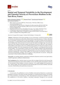
4.2.2. Seasonal Variability To quantify the seasonal variation deeply, monthly average values of TOC from 1978 to 2013 over the YRD for its six latitudinal bands are calculated and shown in Figure 7. The seasonal variation presents a nearly perfect sinusoidal wave with the maximum value in April or May and the minimum in October or November. In analyzing the seasonal variability, this section takes the 31.5°N latitude band as an example. As can be seen from Figure 7, there is an apparent increase in winter and decrease in late spring/summer. The TOC reaches its maximum of 318 DU in April and minimum of 277 DU in October. Seasonal change is 41 DU, which is about 13.9% of the mean value of 296 DU. The seasonal variability is attributed to the photochemical factors and the dynamic factors [39]. Solar radiation is like a double-edged sword for the atmospheric ozone because it is one of the major driving forces for both its production and destruction. Ozone is produced predominantly in the tropics [52–54]; photochemical reactions accelerated by the high-intensity solar radiation lead to the production of ozone. However, the TOC in the tropics is very low all year round [21] because Brewer-Dobson circulation transports the ozone from low latitudes to higher latitude areas [40]. Therefore, it is not surprising to see that there is an increase of TOC from last November to this April in YRD mainly because in this period the transport of Brewer-Dobson circulation is dominant. The decline of TOC in YRD from April to October should be due to the increasing solar radiation and the decrease of the transport in the northern hemisphere [29]. In the mid-latitude region, the photochemical reactions catalyzed by solar incident accelerated the destruction of ozone. In Figure 7, we can also find that the TOC value is larger at higher latitudes than at lower latitudes, especially from December to April. This may be related to the larger planetary-wave amplitudes, which are modulated by the tropical zonal winds. The tropical zonal winds have considerable inertia because of the flywheel effect [52,55]. Figure 7. The monthly average of TOC over the Yangtze River Delta for six latitudinal bands.
340
Total Ozone Column (DU)
330 320 310 300
Lat.33.5°N Lat.32.5°N Lat.31.5°N Lat.30.5°N Lat.29.5°N Lat.28.5°N
290 280 270 260
250 240 Jan Feb Mar Apr May Jun Jul Aug Sep Oct Nov Dec Month
Remote Sens. 2014, 6
12538
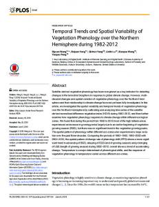
4.2.3. Short-Term Variability To analyze the short-term variability, DDV is calculated for each latitudinal band. The monthly mean DDV for each band from 28.5°N to 33.5°N is shown in Figure 8. It can be seen that the trend of each band presents a notable annual cycle, with the maximum in February and the minimum in August or September. The DDV values of almost all months decrease from February to August or September, and then increase from August or September to the next February. Besides, the DDV in northern latitudes is slightly larger than in southern latitudes for all months (except August). The difference between 33.5°N and 28.5°N ranges between 0.1% (August) and 2.1% (February). These day-to-day evolutions of TOC are mainly caused by tropospheric weather patterns [8,56,57]. The total ozone is higher in the rear and near the center of surface low-pressure systems, while it is lower near surface high-pressure systems. Therefore, the day-to-day changes are related to these dynamical parameters: the free tropospheric temperature, the lower stratospheric temperature [52], the geopotential height [44], the tropopause height [58,59], and the potential vorticity of the lower stratosphere [60]. Figure 8 also shows that the dynamical variability in winter is stronger than in summer. The short-term variations of the TOC reveal a short system memory of the ozone in the Earth’s atmosphere. This system memory is sometimes persistent, which can be useful for predicting the TOC variation. In order to characterize the system memory over the Yangtze River Delta, the temporal autocorrelation coefficients (TAC) (Equation (4)) were calculated with a time lag up to 400 days. Figure 8. The monthly average day-to-day variability (DDV) for the six latitudinal bands over the Yangtze River Delta from 1978 to 2013. 7 6
DDV (%)
5 4
Lat.33.5°N Lat.32.5°N Lat.31.5°N Lat.30.5°N Lat.29.5°N Lat.28.5°N
3 2 1 0
Jan Feb Mar Apr May Jun Jul Aug Sep Oct Nov Dec Month
Two TAC series were calculated based on original and residual TOC series, respectively. Figure 9 shows the evolution of TAC values for the original and residual TOC series in the 31.5°N latitude band. There is a noticeable difference between the two series. In the original series, a fast decrease of the TAC within 12 days is observed. It also can be seen that this decrease begins to slow down and stabilize at 12–26 days. After 26 days, the TAC for the original series decrease almost linearly. In order to measure
Remote Sens. 2014, 6
12539
the TOC system persistence, some other ozone persistence studies define a decorrelation benchmark as 1/e (“e” refers to the base of natural logarithms) [38,40]. From Figure 9, the TAC values decrease to 1/e after 40 days, which indicates that the corresponding time lag and the TOC system persistence is about six weeks. After this, the TAC is nearly zero at a time lag of 103 days, and then reaches its minimum around −1/e at 195 days. From then on, TAC starts to increase, reaching zero at 278 days, +1/e at 377 days. For residual series, the declining rate of TAC is faster than original series within the first 12 days. It decreases rapidly below the 1/e within five days, and to below 0.1 within 29 days. After 29 days, the trend becomes stable with a range of ±0.1. These differences indicate that our methods in Section 4.2.1 (detrending and deseasonalizing the TOC series) are valid, and the deviation of residual autocorrelation coefficients series is mainly related to climatic and dynamic factors. Figure 9. Autocorrelation coefficients of the daily TOC series and residual series with a time lag of up to 400 days (latitudinal band of 31.5°N). 1 Original Ozone series Residual Ozone Series +1/e -1/e
Temporal Autocorrelation Coefficient
0.8 0.6 0.4 0.2 0 -0.2 -0.4 -0.6 Time lag (Days)
5. Conclusions The main purpose of this study was to understand the spatiotemporal variability of total ozone using satellite data (TOMS and OMI) over the Yangtze River Delta for the period 1978–2013. The results of this study can be summarized as follows: For the spatial variability, the latitudinal variability is significant ranging between 3% and 13%, and it also represents an annual cycle with a maximum in February or March and a minimum in August or September. In contrast, the longitudinal variability is less significant; it varies between 2% and 4%. The annual cycle in longitudinal variability can also be easily identified. The long-term trend represents a notable decline for the period 1978–2013 and two sub-periods (1978–1999 and 2004–2013). The ozone depletion is significant during 1978–1999, with a linear trend from (−3.2 ± 0.7) DU/decade to (−10.5 ± 0.9) DU/decade. By contrast, the decrease of ozone during 2004–2013 is not clear. The trend of whole time series still declines at (−1.8 ±0.4) DU/decade. For seasonal variability, a distinct seasonal signature on TOC is found, with a maximum in April or May and a minimum in October or November. This seasonal cycle is also affected by solar radiation and photochemical factors.
Remote Sens. 2014, 6
12540
The day-to-day changes have demonstrated a significant seasonal cycle, with a maximum in February and a minimum in August or September. This is related to tropospheric weather patterns including the free tropospheric temperature, the lower stratospheric temperature, the geopotential height, the tropopause height, and the potential vorticity of the lowermost stratosphere. The TOC system persistence can last about six weeks; after that, autocorrelation coefficients gradually drop to minimal. Acknowledgments This study is supported by the National Natural Science Foundation of China (Grant No.41471449), the National Basic Research Program of China (973 Program) (Grant No. 2010CB951603), and the Fundamental Research Funds for the Central Universities of China. We thank Dr. Qun Yue from East China Normal University for the constructive suggestions. Author Contributions Bailang Yu and Jianping Wu conceived and supervised this study. Liujia Chen and Bailang Yu designed the data processing procedures. Liujia Chen and Zuoqi Chen processed the data. Liujia Chen, Bailang Yu, and Bailiang Li analyzed the results and wrote the paper. Conflicts of Interest The authors declare no conflict of interest. References 1. 2. 3. 4. 5. 6. 7. 8.
9.
Cornu, A. Observation de la limite ultraviolette du spectre solaire adiverses altitudes. CR Hebd. Seances Acad. Sci. 1879, 89, 808. Molina, M.J.; Rowland, F.S. Stratospheric sink for chlorofluoromethanes: Chlorine atom-catalysed destruction of ozone. Nature 1974, 249, 810–812. Rowland, F.; Molina, M.J. Chlorofluoromethanes in the environment. Rev. Geophys. 1975, 13, 1–35. Farman, J.; Gardiner, B.; Shanklin, J. Large losses of total ozone in antarctica reveal seasonal clox/nox interaction. Nature 1985, 315, 207–210. Stolarski, R.S.; Krueger, A.J.; Schoeberl, M.R.; McPeters, R.D.; Newman, P.A.; Alpert, J. Nimbus 7 satellite measurements of the springtime antarctic ozone decrease. Nature 1986, 322, 808–811. Bojkov, R.; Bishop, L.; Hill, W.; Reinsel, G.; Tiao, G. A statistical trend analysis of revised dobson total ozone data over the northern hemisphere. J. Geophys. Res.: Atmos. 1990, 95, 9785–9807. Atkinson, R.J.; Matthews, W.A.; Newman, P.A.; Plumb, R.A. Evidence of the mid-latitude impact of antarctic ozone depletion. Nature 1989, 340, 290–294. Staehelin, J.; Renaud, A.; Bader, J.; McPeters, R.; Viatte, P.; Hoegger, B.; Bugnion, V.; Giroud, M.; Schill, H. Total ozone series at Arosa (Switzerland): Homogenization and data comparison. J. Geophys. Res.: Atmos. 1998, 103, 5827–5841. Varotsos, C.A.; Cracknell, A.P.; Tzanis, C. The exceptional ozone depletion over the arctic in January–March 2011. Remote Sens. Lett. 2012, 3, 343–352.
Remote Sens. 2014, 6
12541
10. Svendby, T.; Dahlback, A. Statistical analysis of total ozone measurements in Oslo, Norway, 1978–1998. J. Geophys. Res.: Atmos. 2004, 109, D16107. 11. Ganguly, N.D.; Tzanis, C. Study of stratosphere-troposphere exchange events of ozone in India and greece using ozonesonde ascents. Meteorol. Appl. 2011, 18, 467–474. 12. Varotsos, C.; Milinevsky, G.; Grytsai, A.; Efstathiou, M.; Tzanis, C. Scaling effect in planetary waves over Antarctica. Int. J. Remote Sens. 2008, 29, 2697–2704. 13. Madronich, S.; McKenzie, R.L.; Björn, L.O.; Caldwell, M.M. Changes in biologically active ultraviolet radiation reaching the Earth’s surface. J. Photochem. Photobiol. B: Biol. 1998, 46, 5–19. 14. Longstreth, J.; de Gruijl, F.; Kripke, M.; Abseck, S.; Arnold, F.; Slaper, H.; Velders, G.; Takizawa, Y.; van der Leun, J. Health risks. J. Photochem. Photobiol. B: Biol. 1998, 46, 20–39. 15. Kondratyev, K.Y.; Varotsos, C.A. Global total ozone dynamics. Environ. Sci. Poll. Res. 1996, 3, 153–157. 16. WMO, W. Scientific Assessment of Ozone Depletion: 2006; Global Ozone Research and Monitoring Project–Report; World Meteorological Organisation, Geneva, Switzerland, 2007; Volume 50, p. 572. 17. Caldwell, M.M.; Björn, L.O.; Bornman, J.F.; Flint, S.D.; Kulandaivelu, G.; Teramura, A.H.; Tevini, M. Effects of increased solar ultraviolet radiation on terrestrial ecosystems. J. Photochem. Photobiol. B: Biol. 1998, 46, 40–52. 18. Ziemke, J.R.; Chandra, S.; Bhartia, P.K. A 25-year data record of atmospheric ozone in the pacific from total ozone mapping spectrometer (toms) cloud slicing: Implications for ozone trends in the stratosphere and troposphere. J. Geophys. Res.-Atmos. 2005, 110, D15105. 19. Staehelin, J.; Harris, N.; Appenzeller, C.; Eberhard, J. Ozone trends: A review. Rev. Geophys. 2001, 39, 231–290. 20. Houghton, J.T. Climate Change 1995: The Science of Climate Change: Contribution of Working Group I to the Second Assessment Report of the Intergovernmental Panel on Climate Change; Cambridge University Press: Cambridge, UK, 1996; Volume 2. 21. Bowman, K.P.; Krueger, A.J. A global climatology of total ozone from the Nimbus 7 total ozone mapping spectrometer. J. Geophys. Res.: Atmos. 1985, 90, 7967–7976. 22. Fahey, D.W.; Hegglin, M.I. Twenty Questions and Answers about the Ozone Layer 2010 Update: Scientific Assessment of Ozone Depletion 2010; World Meteorological Organisation: Geneva, Switzerland, 2011. 23. Hoffmann, M.J. Ozone Depletion and Climate Change: Constructing a Global Response; SUNY Press: New York, NY, USA, 2012. 24. Cheng, Z.; Wang, S.; Jiang, J.; Fu, Q.; Chen, C.; Xu, B.; Yu, J.; Fu, X.; Hao, J. Long-term trend of haze pollution and impact of particulate matter in the Yangtze River Delta, China. Environ. Poll. 2013, 182, 101–110. 25. Stolarski, R.S.; Bloomfield, P.; McPeters, R.D.; Herman, J.R. Total ozone trends deduced from Nimbus 7 TOMS data. Geophys. Res. Lett. 1991, 18, 1015–1018. 26. Herman, J.; Hudson, R.; McPeters, R.; Stolarski, R.; Ahmad, Z.; Gu, X.Y.; Taylor, S.; Wellemeyer, C. A new self-calibration method applied to toms and sbuv backscattered ultraviolet data to determine long-term global ozone change. J. Geophys. Res.: Atmos. (1984–2012) 1991, 96, 7531–7545.
Remote Sens. 2014, 6
12542
27. Fioletov, V.; Bodeker, G.; Miller, A.; McPeters, R.; Stolarski, R. Global and zonal total ozone variations estimated from ground-based and satellite measurements: 1964–2000. J. Geophys. Res.: Atmos. 2002, 107, ACH 21-21–ACH 21-14. 28. Fioletov, V.E.; Shepherd, T.G. Summertime total ozone variations over middle and polar latitudes. Geophys. Res. Lett. 2005, 32, L04807. 29. Antón, M.; Bortoli, D.; Costa, M.J.; Kulkarni, P.S.; Domingues, A.F.; Barriopedro, D.; Serrano, A.; Silva, A.M. Temporal and spatial variabilities of total ozone column over Portugal. Remote Sens. Environ. 2011, 115, 855–863. 30. Chen, Z.; Yu, B.; Huang, Y.; Hu, Y.; Lin, H.; Wu, J. Validation of total ozone column derived from OMPS using ground-based spectroradiometer measurements. Remote Sens. Lett. 2013, 4, 937–945. 31. Total, C. WMO Greenhouse Gas Bulletin. Available online: https://www.wmo.int/pages/ mediacentre/press_releases/documents/GHG_Bulletin_No.8_en.pdf (13 November 2014). 32. NASA Ozone & Air Quality. Available online: http://ozoneaq.gsfc.nasa.gov/index.md (10 December 2013). 33. Tandon, A.; Attri, A.K. Trends in total ozone column over India: 1979–2008. Atmos. Environ. 2011, 45, 1648–1654. 34. Levelt, P.F.; van den Oord, G.H.; Dobber, M.R.; Malkki, A.; Visser, H.; de Vries, J.; Stammes, P.; Lundell, J.O.; Saari, H. The ozone monitoring instrument. IEEE Trans. Geosci. Remote Sens. 2006, 44, 1093–1101. 35. Kroon, M.; Petropavlovskikh, I.; Shetter, R.; Hall, S.; Ullmann, K.; Veefkind, J.; McPeters, R.; Browell, E.; Levelt, P. Omi total ozone column validation with Aura-AVE CAFS observations. J. Geophys. Res.: Atmos. 2008, 113, D15S13. 36. Kroon, M.; Veefkind, J.P.; Sneep, M.; McPeters, R.D.; Bhartia, P.K.; Levelt, P.F. Comparing OMI-TOMS and OMI-DOAS total ozone column data. J. Geophys. Res.-Atmos. 2008, 113, D16S28. 37. Fioletov, V.E.; Labow, G.; Evans, R.; Hare, E.W.; Köhler, U.; McElroy, C.T.; Miyagawa, K.; Redondas, A.; Savastiouk, V.; Shalamyansky, A.M.; et al. Performance of the ground-based total ozone network assessed using satellite data. J. Geophys. Res.: Atmos. 2008, 113, D14313. 38. Schmalwieser, A.W.; Schauberger, G.; Janouch, M. Temporal and spatial variability of total ozone content over central Europe: Analysis in respect to the biological effect on plants. Agric. For. Meteorol. 2003, 120, 9–26. 39. Aesawy, A.; Mayhoub, A.; Sharobim, W. Seasonal variation of photochemical and dynamical components of ozone in subtropical regions. Theor. Appl. Climatol. 1994, 49, 241–247. 40. Chen, D.; Nunez, M. Temporal and spatial variability of total ozone in Southwest Sweden revealed by two ground-based instruments. Int. J. Climatol. 1998, 18, 1237–1246. 41. Hadjinicolaou, P.; Jrrar, A.; Pyle, J.A.; Bishop, L. The dynamically driven long-term trend in stratospheric ozone over northern middle latitudes. Q. J. R. Meteorol. Soc. 2002, 128, 1393–1412. 42. Bowman, K.P. Global patterns of the quasi-biennial oscillation in total ozone. J. Atmos. Sci. 1989, 46, 3328–3343. 43. Zerefos, C.S.; Bais, A.F.; Ziomas, I.C.; Bojkov, R.D. On the relative importance of quasi-biennial oscillation and El Nino/southern oscillation in the revised dobson total ozone records. J. Geophys. Res.: Atmos. (1984–2012) 1992, 97, 10135–10144.
Remote Sens. 2014, 6
12543
44. Ziemke, J.; Chandra, S.; McPeters, R.; Newman, P. Dynamical proxies of column ozone with applications to global trend models. J. Geophys. Res.: Atmos. 1997, 102, 6117–6129. 45. Hadjinicolaou, P.; Pyle, J.; Harris, N. The recent turnaround in stratospheric ozone over northern middle latitudes: A dynamical modeling perspective. Geophys. Res. Lett. 2005, 32, L12821. 46. Harris, N.R.; Kyrö, E.; Staehelin, J.; Brunner, D.; Andersen, S.-B.; Godin-Beekmann, S.; Dhomse, S.; Hadjinicolaou, P.; Hansen, G.; Isaksen, I. Ozone trends at northern mid- and high latitudes—A European perspective. Ann. Geophys. 2008, 26, 1207–1220. 47. Robock, A. The climatic aftermath. Science 2002, 295, 1242–1244. 48. Tourpali, K.; Schuurmans, C.; van Dorland, R.; Steil, B.; Brühl, C. Stratospheric and tropospheric response to enhanced solar UV radiation: A model study. Geophys. Res. Lett. 2003, 30, 1231. 49. Camp, C.D.; Tung, K.-K. The influence of the solar cycle and QBO on the late-winter stratospheric polar vortex. J. Atmos. Sci. 2007, 64, 1267–1283. 50. Ziemke, J.R.; Chandra, S. Development of a climate record of tropospheric and stratospheric column ozone from satellite remote sensing: Evidence of an early recovery of global stratospheric ozone. Atmos. Chem. Phys. 2012, 12, 5737–5753. 51. Solomon, S. Stratospheric ozone depletion: A review of concepts and history. Rev. Geophys. 1999, 37, 275–316. 52. Tung, K.K.; Yang, H. Dynamic variability of column ozone. J. Geophys. Res.: Atmos. 1988, 93, 11123–11128. 53. Bojkov, R.D.; Fieoletov, V.E. Total ozone variations in the tropical belt: An application for quality of ground based measurements. Meteorol. Atmos. Phys. 1996, 58, 223–240. 54. Silva, A.A. A quarter century of TOMS total column ozone measurements over Brazil. J. Atmos. Solar-Terrestr. Phys. 2007, 69, 1447–1458. 55. Scott, R.; Haynes, P. Internal interannual variability of the extratropical stratospheric circulation: The low-latitude flywheel. Q. J. R. Meteorol. Soc. 1998, 124, 2149–2173. 56. Dobson, G.M.; Harrison, D.; Lawrence, J. Measurements of the amount of ozone in the Earth’s atmosphere and its relation to other geophysical conditions. Part III. Proc. R.Soc. Lond. Ser. A 1929, 122, 456–486. 57. Reed, R.J. The role of vertical motions in ozone-weather relationships. J. Meteorol. 1950, 7, 263–267. 58. Bethan, S.; Vaughan, G.; Reid, S. A comparison of ozone and thermal tropopause heights and the impact of tropopause definition on quantifying the ozone content of the troposphere. Q. J. R. Meteorol. Soc. 1996, 122, 929–944. 59. Steinbrecht, W.; Claude, H.; Köhler, U.; Hoinka, K. Correlations between tropopause height and total ozone: Implications for long-term changes. J. Geophys. Res.: Atmos. 1998, 103, 19183–19192. 60. Vaughan, G.; Price, J. On the relation between total ozone and meteorology. Q. J. R. Meteorol. Soc. 1991, 117, 1281–1298. © 2014 by the authors; licensee MDPI, Basel, Switzerland. This article is an open access article distributed under the terms and conditions of the Creative Commons Attribution license (http://creativecommons.org/licenses/by/4.0/).