Investigation on an EM Framework for Partial Volume Image Segmentation Daria Eremina*1,2, Xiang Li3, Wei Zhu2, Jing Wang1,4, and Zhengrong Liang1,4
Departments of Radiology1, Applied Mathematics & Statistics2, and Physics & Astronomy4, State University of New York, Stony Brook, NY 11794, USA Department of Radiation Oncology3, University of Pittsburgh Medical Center, Pittsburgh, PA 15232, USA ABSTRACT This work investigates a new partial volume (PV) image segmentation framework with comparison to a previous PV approach. The new framework utilizes an expectation-maximization (EM) algorithm to estimate simultaneously (1) tissue fractions in each image voxel and (2) statistical model parameters of the image data under the principle of maximum a posteriori probability (MAP). The previous EM approach models the PV effect by down-sampling a voxel and then labels each subvoxel as a pure tissue type, where the number of subvoxels labeled by a given tissue type over the total number of subvoxels reflects the fraction of that tissue type inside the original voxel. The tissue fractions in each voxel in this discrete PV model are represented by a limited number of percentage values. In the new MAPEM approach, the PV effect is modeled in a continuous space and estimated directly as the fraction of each tissue type in the original voxel. The previous discrete PV model would converge to the proposed continuous PV tissue-mixture model if there is an infinite number of subvoxels within a voxel. However, in practice a voxel is usually downsampled once or twice for computational reasons. A simulation study reveals that the continuous PV model is not only more realistic but also more accurate than the discrete PV model. Keywords: PV effect, EM algorithm, parameter estimation, tissue mixture, MAP image segmentation.
1. INTRODUCTION The traditional image segmentation algorithm clusters all the image voxels into several groups and assigns a different label to a corresponding group, where the label indicates a specific tissue type for the voxels inside that group. Due to the limited spatial resolution of the imaging equipment, not all voxels in the labeled group contain the same tissue type, especially for voxels near the tissue borders which are highly likely to contain more than one tissue types. This partial volume (PV) effect causes a significant error in the traditional hard image segmentation. Some improvement has been achieved by soft image segmentation, which determines the probability or likelihood of a tissue label belonging to a voxel in the corresponding group [1-4]. These methods reduced the PV effect, however, they used discrete tissue labeling of a voxel, thus the improvement of the segmentation result was limited. Directly partitioning different tissue percentages by PV image segmentation inside each voxel is desired and has been a challenging task due to insufficient measurements to determine the percentages of different tissue types in each voxel [5-8]. Recently, Leemput et al. [9] presented a PV image segmentation algorithm that directly computes the tissue components in each voxel by downsampling the voxel. For example, a voxel may be halved in three dimentions, resulting in eight subvoxels. These eight subvoxels are labeled in a similar manner as in the traditional hard segmentation. If four subvoxels are labeled as tissue type 1, two as tissue type 2, and the remaining two as tissue type 3, then 50% of the original voxel contains tissue type 1, 25% contains tissue type 2 and 25% contains tissue type 3. Theoretically, this discrete PV image segmentation would converge to the most accurate solution when the down-sampling is repeated infinite times and infinite numbers of labels are used to characterize the down-sampled subvoxels, although in practice, such is not attainable. Here we propose a more accurate continuous PV modeling approach [10]. Comparisons are made to the discrete PV modeling approach [9] via a simulation study. *
Email:
[email protected]; Phone: (631) 444 7921; Fax: (631) 444 6450. Medical Imaging 2006: Image Processing, edited by Joseph M. Reinhardt, Josien P. W. Pluim, Proc. of SPIE Vol. 6144, 61444D, (2006) · 0277-786X/06/$15 · doi: 10.1117/12.653843
Proc. of SPIE Vol. 6144 61444D-1
2. METHODS We assume that the acquired image Y reflects the distribution of K tissue types inside the body. Within each voxel, there are K possible tissue types, where each tissue type has a contribution to the observed voxel value Yi at voxel i. The observed voxel value at each voxel is modeled as a Gaussian random variable with mean Yi and variance σ i2 . This assumption was also taken in other related works [5-9]. We assume further that the intensities of different voxels are independent and the joint distribution of an image is
∏
f ( Y | {Yi }, {σ i2 }) =
I i =1
f (Yi | Yi , σ i2 ) .
(1)
We model each image voxel intensities { Y i , i = 1 , K , I } as a sum of participating pure tissue components in that voxel { X ik , i = 1, K , I ; k = 1, K , K } , where I is the total number of voxels in the image. That is
Yi =
∑
K k =1
X ik .
(2)
Here {Y i } are the acquired image data, which are incomplete to describe fully the underlining tissue types, and {X ik } are unobservable variables, which describe completely the underlining tissue types. Equation (2) was also used in [9], where X ik reflects the down-sampled voxel intensities. All pure tissue-type variables {X ik } are assumed to be independent. We further assume that each unobservable variable X ik follows a Gaussian distribution with mean Z ik µ k and variance Z ik σ k2 , where µ k and σ k2 represent the mean and variance, respectively, of a voxel fully filled
with tissue type k, and Z ik reflects the fraction of tissue type k in voxel i with conditions of
∑
K k =1
Z ik = 1 and
0 ≤ Z ik ≤ 1 . These definitions of mean Z ik µ k and variance Z ik σ were verified mathematically in [9] for their discrete PV model. In the proposed continuous PV model, the joint probability is ⎧ ( X ik − Z ik µ k ) 2 ⎫ I ,K I ,K 1 (3) f ( Χ | { µ k }, {σ k2 }, { Z ik }) = ∏ i , k =1 f ( Χ ik | µ k , σ k2 , Z ik ) = ∏ i , k =1 exp ⎨ − ⎬. 2 Z ik σ k2 2π Z ik σ k2 ⎭ ⎩ 2 k
Based on the above assumptions, we model each image voxel observation Yi as a sum of pure tissue components plus noise, that is,
Y i = Yi + ε i =
∑
K k =1
Z ik µ k + ε i ,
(4)
where ε i represents the Gaussian noise with zero mean and variance of σ I2 = ∑ Z ik σ k2 . k =1 K
Equation (1) then
becomes: f ( Υ | { µ k }, {σ k2 }, { Z ik }) =
∏
1
I i =1
2π
∑
K k =1
Z ik σ
2 k
∑ ∑
⎧ (Y − i ⎪ exp ⎨ − 2 ⎪⎩
Z ik σ k2 ) 2 ⎫⎪ ⎬. . 2 Z σ ⎪⎭ k k =1 ik K
k =1 K
(5)
The maximum likelihood (ML) and penalized ML (pML) or maximum a posteriori probability (MAP) solutions on the incomplete data Gaussian distribution { Yi } of equation (5) for fractions { Z ik } can be computed, given the model parameters { µ k , σ k2 }. In this case, solving the optimization problem can be very complicated because the simultaneous estimation of both the fractions and the model parameters is numerically intractable. To estimate the tissue fractions { Z ik } and tissue model parameters { µ k , σ k2 } simultaneously, we adapt the EM algorithm [11]. The basic ideas of this MAP-EM framework for simultaneous parameter estimation and tissue mixture segmentation were presented in [10]. The mathematical details are given below. An alternative strategy was described in [12, 13], in which equation (5) was directly maximized by the iterated condition mode (ICM) calculation for the fractions { Z ik }
Proc. of SPIE Vol. 6144 61444D-2
while the model parameters { µ k , σ k2 } were updated within each ICM iteration by the EM algorithm, i.e., a hybrid approach. In order to account for the neighborhood information we introduce a Markov random field (MRF) penalty term to define a prior distribution for the fractions in the objective cost function of the MAP-EM framework [10]. The MRF distribution has a general form of (6) f ( Z ik ) = C − 1 × exp[ 12 U ( Z ik )] where the energy function in our case is
U ( Z ik ) = β ∑ r∈ε w ir ⋅ ( Z ik − Z rk ) 2
(7)
i
and {wir } is a set of different weighting factors for different orders of neighbors. In our PV image segmentation algorithm, we used the second-order neighborhood. Our a priori model is similar to the model C in Leemput et al. [9], where several alternative models were reported. Our MAP-EM algorithm for simultaneous estimation of tissue fractions and tissue model parameters consists of the following two steps below. (1). E-step: the conditional expectation is calculated, via equations (3) and (6) at the n-th iteration, by Q (Θ | Θ ( n ) ) = E[ln f ( X | Θ ) f ( Z ) | Y , Θ ( n ) ] =−
1 2
∑ {ln( 2π ) + ln( Z
ik
σ k2 ) +
i ,k
1 Z ik σ
2 k
(8)
[( X ik2 ) ( n ) − 2 X ik( n ) Z ik µ k + Z ik2 µ k2 ] + U ( Z ik )}
where parameter set Θ represents the fractions {Z ik } and tissue parameters {µ k , σ k2 } , and X ik(n ) and ( X ik2 ) ( n )
are the conditional expectations of X ik and X ik2 respectively, X ik( n ) = E[ X ik | Yi , Θ ( n ) ] = Z ik( n ) µ k( n ) +
( Z ik σ k2 ) ( n ) K ⋅ (Yi − ∑ j =1 Z ij( n ) µ (j n ) ) 2 (n) K ∑ j =1 ( Z ij σ j )
( X ik2 ) ( n ) = E [ X ik2 | Y i , Θ ( n ) ] = ( X ik( n ) ) 2 + ( Z ik σ k2 ) ( n ) ⋅ ( n) 2 ik
where ( X ) is the square of the n-th iterated estimate of X
(n ) ik
∑ ∑
K j≠k K j =1
( Z ij σ ) 2 j
(9) (n)
( Z ij σ 2j ) ( n )
.
(10)
.
(2). M-step: the maximization of the conditional expectation determines the (n+1)-th iterated results for fractions and model parameters. For the mean parameter µ k , we have
∑X ∑Z
(n) ik
.
(11)
( X ik2 ) ( n ) − 2 X ik( n ) Z ik( n ) µ k( n ) + ( Z ik2 µ k2 ) ( n ) . Z ik( n )
(12)
µ k( n +1) =
i
i
ik
Similarly for the variance parameter σ k2 , we have (σ k2 ) ( n +1) =
1 I
∑ i
For mixture of two tissue types in each voxel, the fractions { Z ik } can be estimated by the following Z i(1n + 1 ) =
X i(1n ) (σ i22 ) ( n ) µ 1
(n)
+ ( µ 22 ) ( n ) (σ i21 ) ( n ) − X i(2n ) (σ i21 ) ( n ) µ 2
(n)
+ 4 β (σ i21 ) ( n ) (σ i22 ) ( n ) ∑ w ir Z r 1
( µ 12 ) ( n ) (σ i22 ) ( n ) + ( µ 22 ) ( n ) (σ i21 ) ( n ) + 4 β (σ i21 ) ( n ) (σ i22 ) ( n ) ∑ w ir
Proc. of SPIE Vol. 6144 61444D-3
(13)
where Z i(2n+1) = 1 − Z i(1n+1) and σ ik2 = Z ik σ k2 . Tissue mixtures of more than two types in each image voxel will not be considered in this paper for simplicity. The problem to find a solution in these cases of more than two tissue types in each voxel can be solved by using multi-spectral images of the same object such as in the case of magnetic resonance imaging (MRI) which can provide T1, T2 and proton density images. In practice, the number of voxels containing more than two tissue types is relatively small as compared to the total number of voxels in the image. In such cases, approximated calculations of the fractions { Z ik } can be found in the Appendix and also in [5, 11, 12]. Equations (11)-(13) represent the MAP-EM parameter estimation for the continuous PV model. In the special case of a single tissue type, Z i 1 = 1 . From equations (9) and (10), we have the conditional expectation of the only tissue type X i(1n ) = Yi and ( X i21 ) ( n ) = Y i . Also equations (11) and (12) become µ 1( n +1) = µ 1 =
∑Y i
I
i
and
(σ 12 ) ( n +1) = σ 12 =
∑
i
(Y i − µ 1 ) 2 I
.
(14)
These results concur with our expectations. The main difference between the above presented MAP-EM framework and the alternative hybrid algorithm [11, 12] lies in the estimation of fractions (13). Both the presented framework and the hybrid strategy utilize the same EM algorithm for estimating the model parameters and, therefore, share the common equations (11) and (12). However, in the hybrid approach, equation (5) is maximized directly instead of than the cost function of (8) in the EM domain. For two tissue-type case, the maximization results in the following solution for the tissue fractions Z i(1n +1) =
(Yi − µ 2( n ) )( µ 1( n ) − µ 2( n ) ) + 2 β (σ i2 ) ( n ) ∑ wir Z r(1n ) + 2 β (σ i2 ) ( n ) ∑ wir (1 − Z r( 2n ) ) ( µ 1( n ) − µ 2( n ) ) 2 + 4 β (σ i2 ) ( n ) ∑ wir
(15)
The difference between equation (13) and (15) can be more clearly seen if the penalty team is ignored. Equation (15) does not account for the variance parameter and conditional expectation, while equation (13) does. Thus it is expected that the solution for fraction estimation by the alternative hybrid algorithm, equation (15), could be more sensitive to noise as compared to the presented fully EM solution. For a special case of Yi = µ1( n ) and Yi = µ 2( n ) , equation (15) converges to one and zero respectively, regardless the data statistical information, while equation (13) converges to solution of Z ik( n+1) = Z ik( n ) , which had been determined at the n-th iteration by the conditional expectations and model parameters of means and variances. In the followings, we will focus on the comparison between the above continuous PV model EM algorithm (11)-(13) and the previous discrete PV model [9].
3. RESULTS We implemented both the continuous PV-model MAP-EM algorithm presented above and the previous discrete PVmodel MAP-EM method [9] and compared their performances using simulated two-dimensional (2D) images of 256x256 array size. The digital phantom images have diagonal stripes of two and three tissue types respectively, as seen in Fig. 1 and Fig. 3. The phantom used for Fig. 1 contains two intensity levels of { µ1 = 20 , σ 12 = 4 } and { µ 2 = 40 , σ 22 = 8 }, respectively. The PV effect mainly occurs at the border between these two levels. Each fraction Z i1 or Z i 2 was simulated by applying a Gaussian filter to each corresponding level and then adding them together such that Z i1 + Z i 2 = 1 . Gaussian noise was added with mean Z ik µ k and variance Z ik σ k2 for tissue type k in voxel i. Then the noisy phantom image was obtained by the use of equation (2), satisfying both the continuous and discrete PV models. Similarly the phantom used for Fig. 3 was simulated such that { µ1 = 100 , σ 12 = 5 }, { µ 2 = 150 , σ 22 = 8 }, and { µ3 = 200 , σ 32 = 16 }, respectively. The PV effect at the two borders satisfies Z i1 + Z i 2 + Z i 3 = 1 . These two noise phantom images were segmented by the above presented MAP-EM algorithm and the previously reported one [9]. Both algorithms were implemented by C++ code on a PC platform of 2.0GHz CPU and 1.5GB memory.
Proc. of SPIE Vol. 6144 61444D-4
In implementing the Leemput et al. method [9], each original voxel was divided into four subvoxels, i.e., 2x2 downsampling. The method is computationally complex and intensive due to the Monte Carlo (MC) sampling on the labels of the subvoxels [9]. The computing time was approximately 5 minutes per iteration. The implementation became problematic for 3x3 down-sampling (i.e., each original voxel was divided into nine subvoxels), it took more than three hours to finish one iteration. In addition to the intensive computation, another drawback of method [9] is the segmentation accuracy. For the 2x2 down-sampling, the segmentation accuracy for the tissue fractions is limited to five values: 0%, 25%, 50%, 75% and 100%. In our continuous PV model, the tissue fractions takes any value between zero and one, i.e., 0 ≤ Z ik ≤ 1 . The computing time of our MAP-EM segmentation was less than 1 second per iteration.
(a)
(b)
Fig. 1: Phantom study of two intensity levels: (a) the noisy phantom image; and (b) an initially-estimated fraction image for iterative MAP-EM update.
We used a simple thresholding technique in order to get an initial segmentation of images in order to start the iterative process. We classified voxels from Fig. 1 image (left) into two groups and voxels from Fig. 3 image (left) into three groups respectively. Then the initial estimates of the means { µ k( 0 ) } and variances { σ k2 ( 0 ) } were computed from the classified groups. Finally the initial estimates of the fractions { Z ik( 0 ) } were determined by the ratio of the number of classified voxels in each group within a window of the second order neighborhood to the total number of the voxels in this neighborhood. The initial estimates of the fractions { Z ik( 0 ) } are shown in Fig. 1 (right) for two tissue type image and Fig. 3 (right) for three tissue image. For example, the initial estimates of the model parameters are { µ1 = 19.65 , σ 12 = 5.05 } and { µ 2 = 39.28 , σ 22 = 9.16 } for the two tissue type study, and { µ1 = 100.02 , σ 12 = 12.35 }, { µ 2 = 149.5 , σ 22 = 18.85 }, and { µ 3 = 199.01 , σ 32 = 24 .23 } for the three tissue type study. These initial estimates on the model parameters are very close to the true model values, although the initial estimate of the fractions can be very different from the true mixture values. Therefore, the initial model-parameter estimates were altered away from the true values (to be discussed later). To stop the iterative processes, the criterion of {
∑
| Z
( n + 1) ik
− Z
(n) ik
|} / I ≤ δ
(16)
i,k
was used, where the sum of differences between the value of the fractions at the (n+1)-th iteration and the value of the fractions at the n-th iteration is less than the threshold δ as specified by the user. In this study, the threshold δ was set to be 0.01. The previous method of discrete PV model [9] took 6 iterations to satisfy the stopping criterion, while the presented algorithm took 160 iterations. The advantage of using the digital phantoms is that we know the actual PV compartment of an image and can compare it to the output of the MAP-EM algorithms. The error between the true segmentation and the output of each algorithm is
Proc. of SPIE Vol. 6144 61444D-5
defined as the ratio of differences in fractions of the actual partition and the output of each MAP-EM algorithm to the number of voxels in the image error =
∑
i,k
| Z ikoutput − Z iktrue | I
.
(17)
The results are shown in the Tab. 1 below. Fig. 2 shows the mixture of the central part of the ground true and the segmentation results from the two methods. We ran each algorithm twice. Firstly we did not include the prior on fractions into the model (i.e., β = 0 ) thus did not use the neighborhood information. Then we tested the performance of the algorithms with the prior, β = 0.85 . It can be seen that the performances of both algorithms are similar, but the continuous PV model gives a better segmentation. The neighborhood information improves the segmentation results considerably, which mean that the prior term cannot be omitted. The estimation of tissue parameters was robust for both algorithms. For the previous discrete PV model, the estimated model parameters are { µ1 = 19.43 , σ 12 = 4 } and { µ 2 = 39.42 , σ 22 = 4.0 }. For the current continuous PV model, they are { µ1 = 19.45 , σ 12 = 4.05 } and { µ 2 = 39.55 , σ 22 = 7.58 }.
error
Dis-PV, no prior 1.75%
Cont-PV, no prior 1.17%
Dis-PV, with prior 1.39%
Cont-PV, with prior 1.04%
Tab. 1: Comparison of continuous and discrete PV models in the case of two tissue types.
(a)
(b)
(c)
Fig. 2: Mixture results of the border (a) ground truth; (b) MAP-EM algorithm of discrete PV model; and (c) our new algorithm.
After the phantom study with two tissue types, both algorithms were applied to the phantom data with three tissue types, as seen in Fig. 3. Most of the tissue mixture or PV effect occurs at the borders between two tissues. The quantitative measures on the output of the algorithms are shown in the Tab. 2, where the error is the ratio of miscalculated percentages in the output. The improvement by the continuous PV model over the discrete PV model is again seen. The robust estimation for tissue parameters was observed again for both algorithms. The estimated model parameters are { µ1 = 100.03 , σ 12 = 4 }, { µ 2 = 149.5 , σ 22 = 4 }, and { µ 3 = 199 , σ 32 = 4 } for the discrete PV model, and { µ1 = 99.4 , σ 12 = 4.7 }, { µ 2 = 149.5 , σ 22 = 7.8 }, and { µ 3 = 199.8 , σ 32 = 16.3 } for the continuous PV model.
Proc. of SPIE Vol. 6144 61444D-6
(a)
(b)
Fig. 3: Phantom study of three intensity levels: image for iterative MAP-EM update.
error
(a) the noisy phantom image; and (b) an initially-estimated fraction
Dis-PV, with prior 1.36%
Cont-PV, with prior 1.19%
Tab. 2: Comparison of continuous and discrete PV models in the case of three tissue types.
The above phantom studies with two and three tissue types were repeated with higher noise levels (i.e., nearly double the variance), a similar improved performance on the fraction segmentation of the continuous over the discrete PV models was observed. The estimation of the model parameters remained excellent, similar to the results reported above. The iterative processes of both the continuous and discrete PV models were not sensitive to the initial model parameters. When the initial means and variances were added by 10% more errors, both algorithms still converged to good results. In contrast, the convergence appears to be more sensitive to the initial estimate of the fractions, although further investigation is necessary.
4. DISCUSSION AND CONCLUSION There are many PV algorithms presented in the literature including the well-known methods by Choi et al. [5], which was one of the first in this field, and more recently, Leemput et al. [9], who provided a solution which encompasses several existing PV methods. In their work, Choi et al. [5] introduced a statistical model, which allows multiple tissue types within a voxel. Incorporating spatial information through prior on pure tissue types, they searched the MAP segmentation solution for voxels fractions. The prior information on neighborhood voxels was used in order to improve the results and make the algorithm robust. Leemput et al. [9] proposed another PV segmentation approach based on down-sampling. They utilized the EM framework to model the labels of the down-sampled voxels. In the case of spatial model with MRF prior on the labels, they also accounted for the neighborhood information. Monte Carlo method was used to simulate labels and estimate the covariances in the MRF prior neighborhood voxels probabilities. In this paper we presented a new PV segmentation model, which has several advantages over the previous ones. The main drawback of the algorithm from Choi et al. [5] is that they utilized a heuristic method to estimate the tissue parameters and prior information to assign only one tissue type to a voxel. In our proposed algorithm the estimation of both tissue model parameters and fractions are done consistently through the EM technique. The main advantage of our work over that of Leemput et al. [9] is that our model adopts continuous set of fractions rather than discrete labels. In the discrete PV model [9], the number of subvoxels must be infinitively large for accuracy, which is not attainable even in the simple case of 3x3 down-sampling because of the computational cost. We demonstrated that the results of the proposed continuous PV algorithm are similar in the estimation of the model
Proc. of SPIE Vol. 6144 61444D-7
parameters, but more accurate in the estimation of fraction than Leemput et al. [9]. Furthermore, robust results can be obtained without resorting to the sampling simulation techniques such as Monte Carlo or Gibbs sampler, which are known to be time consuming and thus impractical for clinic purposes. Compared to the previous hybrid strategy [11, 12], the newly presented pure MAP-EM segmentation framework is consistent in theory and more robust to noise. In derivations of equations (13) and (15), their cost functions were approximated by a quadratic form by fixing the variance in the log term and the denominator of equation (8) from the previous iteration. The disadvantage of the proposed method is that it can not account for three and more tissue type mix within a voxel without the use of multi-spectral images or an atlas reference.
APPENDIX In the case of three tissue-type mixture within a voxel, the segmentation solution for the tissue fractions can be found by minimizing the following objective function for each voxel [5, 12, 13], via equation (8), 1 Q = (Z i1 2
Z i2
⎡U 0 Z i 3 )⎢⎢U 3 ⎣⎢U 6
U1 U4 U7
2 (n) where U = ( µ 1 ) + 2 β ∑ wir , U1 = U 2 = U 3 = 0, 0 ( Z i1σ 12 ) ( n ) r ∈ε
U 2 ⎤ ⎛ Z i1 ⎞ ⎜ ⎟ U 5 ⎥⎥ ⎜ Z i 2 ⎟ − (b0 U 8 ⎦⎥ ⎜⎝ Z i 3 ⎟⎠ U4 =
i
( µ 22 ) ( n ) ( Z i 2 σ 22 ) ( n )
b1
⎛ Z i1 ⎞ ⎜ ⎟ b2 )⎜ Z i 2 ⎟ ⎜Z ⎟ ⎝ i3 ⎠
(A.1)
( µ 32 ) ( n ) + 2 β ∑ wir , U 8 = + 2 β ∑ wir , ( Z i 3σ 32 ) ( n ) r∈ε i r∈ε i
(n) (n) (n) (n) (n) (n) U 5 = U 6 = U 7 = 0 and b0 = X i1 µ1 + 2 β ∑ wir Z r(1n ) , b1 = X i 2 µ 2 + 2 β ∑ wir Z r( 2n ) , b2 = X i 3 µ 3 + 2 β ∑ wir Z r(3n ) . 2 (n) 2 (n) ( Z i1σ 1 ) ( Z i 2σ 2 ) ( Z i 3σ 32 ) ( n ) r∈ε i r∈ε i r∈ε i
The solution is obtained by solving the following equation system
⎧Z i1 + Z i 2 + Z i 3 = 1 ⎪ ⎨Z i1 (U 0 − U 1 ) + Z i 2 (U 3 − U 4 ) + Z i 3 (U 6 − U 7 ) = b0 − b1 ⎪Z (U − U ) + Z (U − U ) + Z (U − U ) = b − b 2 i2 3 5 i3 6 8 0 2 ⎩ i1 0
(A.2)
In the case of four tissue type mixture in a voxel, the solution for the tissue fractions is determined by the following equation system
⎧ ⎪Z i1 + Z i 2 + Z i 3 + Z i 4 = 1 ⎪ ⎨Z i1 (U 0 − U 3 ) + Z i 2 (U 1 − U 7 ) + Z i 3 (U 2 − U 11 ) + Z i 4 (U 3 − U 15 ) = b0 − b3 ⎪Z i1 (U 1 − U 3 ) + Z i 2 (U 5 − U 7 ) + Z i 3 (U 6 − U 11 ) + Z i 4 (U 7 − U 15 ) = b1 − b3 ⎪ ⎩Z i1 (U 2 − U 3 ) + Z i 2 (U 6 − U 7 ) + Z i 3 (U 10 − U 11 ) + Z i 4 (U 11 − U 15 ) = b2 − b3
(A.3)
2 (n) ( µ 22 )( n ) ( µ32 )( n ) where U = ( µ 1 ) + 2 β ∑ wir , U1 = U 2 = U 3 = 0, , U 5 = + 2 β ∑ wir , U10 = + 2 β ∑ wir , 0 2 (n) 2 (n) ( Z i 2σ 2 ) ( Z i 3σ 32 )( n ) ( Z i1σ 1 ) r ∈ε r ∈ε r ∈ε i
i
i
(n) (n) (n) (n) ( µ 42 )( n ) , U 6 = U 7 = U11 = 0 and b = X i1 µ1 + 2 β w Z ( n ) , b = X i 2 µ 2 + 2 β w Z ( n ) , U15 = + 2 β w ∑ ∑ ir r 2 ∑ 0 1 ir r 1 ir ( Z i 4σ 42 )( n ) ( Z i1σ 12 ) ( n ) ( Z i 2σ 22 ) ( n ) r ∈ε i r∈ε i r∈ε i
b2 =
X i(3n ) µ 3( n ) X (n) µ (n) + 2 β ∑ wir Z r(3n ) , b3 = i 4 2 4 ( n ) + 2 β ∑ wir Z r( 4n ) . 2 (n) ( Z i 4σ 4 ) ( Z i 3σ 3 ) r ∈ε i r∈ε i
ACKNOWLEDGEMENT This work was supported in part by the NIH National Cancer Institute under Grant # CA082402 and Grant # CA110186.
Proc. of SPIE Vol. 6144 61444D-8
REFERENCES 1. 2. 3. 4. 5. 6. 7. 8. 9. 10. 11. 12. 13.
Z. Liang, R. Jaszczak, and E. Coleman, “Parameter estimation of finite mixtures using the EM algorithm and information criteria with application to medical image processing”, IEEE Transactions on Nuclear Science, vol. 39, pp. 1126-1133, 1992. S. Sanjay-Gopal and T. J. Hebert, “Bayesian pixel classification using spatially variant finite mixtures and the generalized EM algorithm”, IEEE Transactions on Image Processing, vol. 7, pp. 1014-1028, 1998. Y. Zhang, M. Brady, and S. Smith, “Segmentation of brain MR images through a hidden Markov random field model and the expectation-maximization algorithm,” IEEE Transactions on Medical Imaging, vol. 20, pp. 45-57, 2001. L. Li, H. Lu, X. Li, W. Huang, A. Tudorica, C. Christodoulou, L. Krupp, and Z. Liang, “MRI volumetric analysis of multiple sclerosis: methodology and validation”, IEEE Transactions on Nuclear Science, vol. 50, pp. 1686-1692, 2003. H. S. Choi, D. R. Haynor, and Y. Kim, “Partial volume tissue classification of multichannel magnetic resonance images – a mixel model”, IEEE Transactions on Medical Imaging, vol. 10, pp. 395-407, 1991. P. Santago and H. D. Gage, “Quantification of MR brain images by mixture density and partial volume modeling”, IEEE Transactions on Medical Imaging, vol. 12, pp. 566-574, 1993. P. Santago and H. D. Gage, “Statistical models of partial volume effect”, IEEE Transactions on Image Processing, vol. 4, pp. 1531-1539, 1995. K. Blekas, A. Likas, N. P. Galatsanos, and I. E. Lagaris, “A spatially constrained mixture model for image segmentation”, IEEE Transactions on Neural Networks, vol. 16, pp. 494-498, 2005. K. Leemput, F. Maes, D. Vandermeulen, and P. Suetens, “A unifying framework for partial volume segmentation of brain MR images”, IEEE Trans. Medical Imaging, vol. 22, pp. 105-119, 2003. Z. Liang, X. Li, D. Eremina, and L. Li, “An EM framework for segmentation of tissue mixtures from medical images”, International Conference of IEEE Engineering in Medicine and Biology, Concun, Mexico, pp. 682-685, 2003. A. Dempster, N. Laird, and D. Rubin, “Maximum likelihood from incomplete data via the EM algorithm”, J R Stat. Soc., vol. 39B, pp. 1-38, 1977. X. Li, D. Eremina, L. Li, and Z. Liang, “Partial volume segmentation of medical images”, Conference Record of IEEE Nuclear Science Society-Medical Imaging Conference, in CD-ROM, 2003. X. Li, Z. Liang, P. Zhang, and G. Kutcher, “An accurate colon residue detection algorithm with partial volume segmentation”, Proceeding of SPIE Medical Imaging, vol. 5370, pp. 1419-1426, 2004.
Proc. of SPIE Vol. 6144 61444D-9