Abstract. In this paper we use different decimation strategies in irreg- ular pyramid segmentation framework, to produce perceptually impor- tant groupings.
Irregular Pyramid Segmentations with Stochastic Graph Decimation Strategies? Yll Haxhimusa, Adrian Ion, and Walter G. Kropatsch Vienna University of Technology, Faculty of Informatics Pattern Recognition and Image Processing Group {yll,ion,krw}@prip.tuwien.ac.at
Abstract. In this paper we use different decimation strategies in irregular pyramid segmentation framework, to produce perceptually important groupings. These graph decimation strategies, based on the maximum independent set concept, used in Bor˚ uvka’s minimum spanning tree based partitioning method, show similar discrepancy segmentation errors. Global and local consistency error measures do not show big differences between the methods although human visual inspection of the results show advantages for one method. To a certain extent this subjective impression is captured by the new criteria of ’region size variation’.
1
Introduction
It is suggested in [1] to bridge and not to eliminate the representational gap, and to focus efforts on region segmentation, perceptual grouping, and image abstraction. The segmentation process results in ’homogeneous’ regions with respect to the low-level cues using some similarity measures. Problems occur since the homogeneity of low levels does not always lead to semantically plausible regions and the difficulty of defining the degree of homogeneity of a region. Thus, using only low-level vision cues cannot produce a complete final ’good’ segmentation [2], since there is an intrinsic ambiguity in the exact location of region boundaries as well as the problems in defining the context of a digital image. Although the methods that do not use the context of the image cannot produce a ’good’ segmentation, they can be valuable tools in image analysis just like efficient edge detectors are. Hence, the low-level coherence of brightness, color, texture or motion attributes should be used to come up sequentially with partitions [4]. A grouping method should have the following properties [3]: capture perceptually important groupings (encoding global views of an image); be highly efficient (running in time (near) linear), and create hierarchical partitions [4]. Computer vision problems could benefit from an efficient computation of segmentation. Regular image pyramids are an efficient representation for fast grouping and access to image objects in top-down and bottom-up processes. However, it is shown that regular image pyramids are confined to globally defined sampling ?
Supported by the Austrian Science Fund under grants P18716-N13 and S9103-N04.
grids and lack shift invariance [5], and that they have to be rejected as generalpurpose segmentation algorithms. To avoid these drawbacks, [6] proposes irregular image pyramids (adaptive pyramids), where the hierarchical structure of the pyramid is not a priori known but recursively built based on the data. [7] shows that irregular pyramids can be used for segmentation and feature detection. In the same sense, segmentation can be evaluated purely1 as segmentation by comparing the segmentation done by humans with those done by a particular method [9]. There is a consistency of segmentation done by humans, even thought humans segment images at different granularity (refinement or coarsening) (Fig. 2, rows 3 − 4). This refinement or coarsening could be thought of as hierarchical structure of the image, i.e. the pyramid. Thus in [9] a segmentation evaluation framework that does not penalize this granularity is used (Sec. 5). In order to achieve efficiency in image partitioning, Bor˚ uvka’s algorithm[10] is combined with dual graph contraction (DGC) [11] for building in a hierarchical way a minimum weight spanning tree (of the region)(Sec. 3). We use the idea of building a minimum weight spanning tree (MST) to find region borders quickly and effortlessly in a bottom-up way based only on local differences in a specific feature. Different stochastic strategies (MIS, MIES, D3P, Sec. 2) for contraction kernels are used within the DGC, thus yielding different partitioning methods. We evaluate the normalized cut [4](NCutSeg) and the method based on the Bor˚ uvka’s MST [12](Bor˚ uSeg) (all three flavors depending on the decimation strategy used: MIS, MIES or D3P (Bor˚ uSeg (MIS), Bor˚ uSeg (MIES) and Bor˚ uSeg (D3P)). We compare these methods following the framework of [9], and show that the methods have similar discrepancy error. Although, qualitative inspection of the produced segmentations showed differences between the methods which the pixel-based discrepancy measures did not show (Sec. 5).
2
Irregular Graph Pyramid
In a regular image pyramid, the number of pixels at any level k is λ times higher than the number of pixels at the next (reduced) level k + 1. The so called reduction factor λ is greater than one and it is the same for all levels k. If s denotes the number of pixels in an image I, the number of new levels on top of I amounts to logλ (s). This implies that an image pyramid is build in O[log(image diameter)] time [8], as well as algorithms running on this representation (Fig. 1a). An irregular pyramid should be used instead of regular ones for segmentation methods [6]. Irregular pyramids can perform all the operations for which their regular counterparts are employed [13]. Each level represents a partition of the pixel set into cells, i.e.connected subsets of pixels. The construction of an irregular pyramid is iteratively local [14]. On the base level (level 0) of an irregular pyramid the cells represent single pixels and the neighborhood of the cells is defined by the 4(8)-connectivity of the pixels. A cell on level k + 1 (parent) is a union of some neighboring cells on level k (children). This union is controlled by so called contraction kernels (CK) [11]. Every parent computes its values independently 1
The context of the image is not taken into consideration during segmentation.
h
1
Gk
λ 1
λ2 λn
Gk
0 s a) Reduction factor
reduction window b) Discrete levels c) Image to dual graphs (Gk , Gk )
Fig. 1. a,b) Pyramid concept, and c) partition of pixel set into cells and representation of the cells and their neighborhood relations by a dual pair (Gk , Gk ) of plane graphs.
of other cells on the same level. We assume that there is a highest level h. Although adaptive pyramids overcome the drawbacks of their regular ancestors and although they grow to a reasonable height as long as the base is small, they grow higher than the logarithm of base diameter with a larger input size because the progressive deviation from the regular base favors configurations that slow down the contraction process. As a consequence of the greater height the efficiency of pyramids degrades. It is shown in [15] that this problem can be resolved by a new selection mechanism (MIES) which guarantees logarithmic heights. The maximal independent set concept from graph theory is the main principle behind the methods to find the set of CKs: the maximal independent vertex set (MIS)[14]; the maximal independent edge set (MIES) [15] and the data driven decimation process (D3P) [16]. Irregular graph pyramids build by MIS may have a very poor reduction factor and small reduction factors are likely, especially when the images are large [15]. The MIES method guarantees a reduction factor of at least 2.0, proved theoretically, but is applicable only if the edges may be contracted in both directions as in the case of segmentation. The D3P method is proposed to speed up the process of finding the set of CKs. A level of the graph pyramid consists of a pair (Gk , Gk ) of plane graphs Gk and its geometric dual Gk (Fig. 1c). The planarity of graphs restricts us to use only the 4-connectivity of the pixels. The vertices of Gk represent the cells on level k and the edges of Gk represent the neighborhood relations of the cells, depicted with square vertices and dashed edges in Fig. 1c. The edges of Gk represent the borders of the cells on level k, solid lines in Fig. 1c, possibly including so called pseudo edges needed to represent neighborhood relations to a cell completely enclosed by another cell. Finally, the vertices of Gk (circles in Fig. 1c), represent junctions of boundary segments of Gk . Moreover the graph is attributed, G = (V, E, av , ae ), where av : V → R+ is a weighted function defined on vertices and ae : E → R+ is a weighted function defined on edges (similar applies for Gk ). The sequence (Gk , Gk ), 0 ≤ k ≤ h is called irregular (dual) graph pyramid and is build using Alg. 1. For simplicity of the presentation the dual G is omitted afterward.
3
MST based Segmentation Algorithm
The segmentation method is supposed to find natural groupings from the pixel set. It is expected that, the measures of dissimilarity capture the expectation
Algorithm 1 – Constructing Dual Graph Pyramid Input: Graphs (G0 , G0 ) 1: while further abstraction is possible do 2: select contraction kernels by an iterative local method /* use MIS, MIES or D3P to determine contraction kernels */ 3: perform dual graph contraction and simplification of dual graph (DGC [11]) 4: apply reduction functions to compute content of new reduced level Output: Graph pyramid – (Gk , Gk ), 0 ≤ k ≤ h.
that the similarity of pixels within a segment (internal ) is less than the similarity between pixels in different segments (external ). The goal is to find the segments that have strong internal similarities, which optimize the criterion function. The pairwise comparison of neighboring vertices, i.e. partitions, is used to check for similarities [3]. This function measures the difference along the boundary of two components relative to a measure of differences of components’ internal differences, i.e. tries to capture the notion of contrast: a contrasted zone is a region containing two connected components whose inner differences (internal contrast) are less than differences within it’s context (external contrast). Let G = (V, E, av , ae ) be a given attributed graph. The goal is to find partitions P = {C1 , C2 , ..., Cn } such that these elements are disjoint and satisfy certain S properties. Moreover P is a partition of V ∈ G, ∀i 6= j, Ci ∩ Cj = φ and Ci = V , ∀i = 1, ..., n. The graph on level k of the pyramid is denoted by Gk . Every vertex u ∈ Gk is a representative of a component Ci of the partition Pk . The equivalent contraction kernel of a vertex u ∈ Gk , N0,k (u) is a set of edges forming a tree on the base level e ∈ E0 that contracts the subgraph G0 ⊆ G = N0,k (u) onto the vertex u. The internal contrast of the Ci ∈ Pk is the largest dissimilarity of component Ci i.e. the largest edge weight of the N0,k (u) of vertex u ∈ Gk : I(Ci ) = max{ae (e), e ∈ N0,k (u)}.
(1)
Let ui , uj ∈ Vk be the end vertices of an edge e ∈ Ek . The external contrast between two components Ci , Cj ∈ Pk is the smallest dissimilarity between component Ci and Cj i.e. the smallest edge weight connecting the trees N0,k (ui ) and N0,k (uj ) of vertices ui ∈ Ci and uj ∈ Cj : E(Ci , Cj ) = min{ae (e), e = (v, w) : v ∈ N0,k (ui ) ∧ w ∈ N0,k (uj )}.
(2)
The I(Ci ) is the maximum of edge weights of the tree within Ci , whereas E(Ci , Cj ) is the minimum of weights of the edges (bridges) connecting component Ci and Cj on the base level G0 . Vertices ui and uj are representative of the components Ci and Cj . The pairwise comparison function B(·, ·) is defined as: � 1 if E(Ci , Cj ) > P I(Ci , Cj ), B(Ci , Cj ) = (3) 0 otherwise, where P I(·, ·) is the minimum internal contrast between two components, defined as P I(Ci , Cj ) = min(I(Ci ) + τ (Ci ), I(Cj ) + τ (Cj )). For the function B(·, ·) to
Algorithm 2 – Construct Hierarchy of Partitions (Bor˚ uSeg) [12] Input: attributed graph G0 . 1: k ← 0 2: repeat 3: for all vertices u ∈ Gk do 4: Emin (u) ← argmin{ae (e) | e = (u, v) ∈ Ek or e = (v, u) ∈ Ek } 5: Emin = Emin ∪ Emin (u) 6: for all e = (uk,i , uk,j ) ∈ Emin do 7: if P I(Cik , Cjk )−E(Cik , Cjk ) is a strikt local maximum in the edge graph then 8: include edge e in contraction edges Nk,k+1 9: contract graph Gk with contraction kernels, Nk,k+1 : Gk+1 ← C[Gk , Nk,k+1 ]. /* MIS, MIES or D3P used as decimation methods */ 10: for all ek+1 ∈ Gk+1 do 11: set edge attributes ae (ek+1 ) ← min{ae (ek ) | ek+1 = C[ek , Nk,k+1 ]} 12: k ←k+1 13: until Gk = Gk−1 Output: a region adjacency graph (RAG) at each level of the pyramid.
be true, i.e. for the border to exist, the external contrast must be greater than the internal contrast. Note that B(·, ·) is a boolean comparison function and the resulted segmentation is a so called crisp segmentation. Using the comparison function B(·, ·) defined previously one can define the algorithm to build the hierarchy of partitions (Alg. 2). Step 10 of this algorithm is the same as steps 2 − 4 of Alg. 1. For more details on steps of this algorithm see [12]. A threshold function τ (C) is used since for small components C, I(C) is not a good estimate of the local characteristics of the data, in extreme case when |C| = 1, I(C) = 0. Any non-negative function of a single component C can be used for τ (C) [3]. We define τ to be a function of the size of C: τ (C) = α/|C|, where |C| denotes the size of the component C and α is a constant. A large constant α sets the preference for larger components. The size of |C| gets larger as the algorithms proceeds hence τ → 0, i.e. the influence of the parameter decreases.
4
Segmentation Results
We start with the trivial partition, where each pixel (vertex) is a homogeneous region. The attributes of edges can be defined as the difference between end point features of end vertices, ae (ui , uj ) = |F (ui ) − F (uj )|, where F is some feature. F could be defined as F (ui ) = I(ui ), for gray value intensity images, or F (ui ) = [vi , vi · si · sin(hi ), vi · si · cos(hi )], for color images in HSV color distance [4]. However the choice of the definition of the weights and the features to be used is in general a hard problem, since the grouping cues could conflict each other. In order to evaluate the methods in our experiments we choose simple gray intensity difference, i.e. ae (ui , uj ) = |I(ui ) − I(uj )|. Note that the methods are applicable to any color space as well. The segmentation results of NCutSeg2 , 2
See [4] for NCutSeg default parameters, and for all Bor˚ uSeg α is set to 500.
on gray value images are shown in Fig. 2 rows 4-5 of Bor˚ uSeg (MIS) in rows 6-7; of Bor˚ uSeg (MIES) in rows 8-9 and Bor˚ uSeg (D3P) in rows 10-11. These methods use only local contrast based on pixel intensity values. As expected, and shown in Fig. 2, segmentation methods, which are based only on low-level local cues, can not create segmentation results as good as humans. Even thought it looks like, the NCutSeg method produces more regions, actually the overall number of regions in row 4, 6, 8, 10 and 5, 7, 9, 11 are almost the same, but Bor˚ uSeg produces more small regions. Anyway all the methods were capable of segmenting the face of a man satisfactory (image #35). Bor˚ uSeg did not merge the statue on the top of the mountain with the sky (image #17). Humans do segment this statue as a single region (see Fig. 2). All methods have problems segmenting the see creatures (image #12). Note that the segmentation done by humans on the image of rocks (image #18), contains the symmetry axis, even thought there is no ’big’ change in the local contrast, therefore the NCutSeg and Bor˚ uSeg methods fail in this respect. None of the methods is ’looking’ for this axis of symmetry.
5
Evaluation of Segmentations
For the evaluation, real world images should be used, since it is difficult to extrapolate conclusions based on synthetic images to real images [17], and the human should be the the final evaluator. We use the empirical method for the evaluation, which studies properties of the segmentations by measuring how ‘good’ a segmentation is close to an ‘ideal’ one, by measuring this ‘goodness’ with some function of parameters [18]. The difference between the segmented image and the reference (ideal) one is used to asses the performance of the algorithm [18], and measured by a discrepancy method. The reference image could be a synthetic image or manually segmented by humans. Higher value of the discrepancy means bigger error, signaling poor performance of the segmentation method. In [18], it is concluded that evaluation methods based on “mis-segmented pixels should be more powerful than other methods using other measures”. In [9] the error measures used for segmentation evaluation ‘count’ the mis-segmented pixels. Segmentations made by humans are used as a reference for benchmarking segmentations produced by different methods. The idea behind this is the observation that, even though different people produce different segmentations for the same image, the obtained segmentations differ, mostly, only in the local refinement of certain regions. This concept has been studied on the human segmentation database (Fig. 2 row 2 − 3) in [9] and used as a basis for defining two error measures, which do not penalize a segmentation if it is coarser or more refined than another. They define two error measures based on the pixel error measures (local refinement error), that counts miss-classified pixels between two regions of two segmentations: the global consistency error (GCE), which forces all local refinements to be in the same direction; and local consistency error (LCE), which allows refinement in different directions in different parts of the image. GCE is a tougher measure than LCE, because GCE tolerates only simple refinements, while LCE tolerates mutual refinement as well. We use the
Original Human segmentation
1
2
3
NCutSeg
4
MSTBor˚ uSeg(MIS)
5
6
uSeg(MIES) MSTBor˚ uSeg(D3P) MSTBor˚
7
8
9
10
11 #35
#17
#2
#12
#18
Fig. 2. Segmentation of Humans [9], and NCutSeg and MSTBor˚ uSeg methods.
Method vs. Humans
b
Method Humans NCutSeg
µLCE 0.059 0.204 MIES 0.203 Bor˚ uSeg MIS 0.200 D3P 0.215
Humans
b
NCutSeg
160
µGCE 0.083 0.248 0.278 0.273 0.303
b
µGCE = 0.0832
100
60
40
40
20
20 0.2
0.4
0.6
0.8
1
error
160
b
µGCE = 0.2731
100
0 0
b
µGCE = 0.2784
100
60
60
40
40
20
20 0.4
0.6
0.8
Bor˚ uSeg (MIS)
1
error
0 0
0.4
0.6
0.8
1
error
b
µGCE = 0.3034
100
40
0.2
0.2
160
60
0 0
b
µGCE = 0.2485
100
60
0 0 160
160
20 0.2
0.4
0.6
0.8
1
error
Bor˚ uSeg (MIES)
0 0
0.2
0.4
0.6
0.8
1
error
Bor˚ uSeg (D3P)
Fig. 3. Histograms of GCE and summary of LCE and GCE discrepancy errors.
GCE and LCE measures to evaluate the Bor˚ uSeg method using the human segmented images from the Berkley image database [9]. The results of the NCutSeg method vs Humans and Humans vs Humans are confirmed [9]. A segmentation consisting of a single region and a segmentation where each pixel is a region, is the coarsest and finest possible of any segmentation. In this sense, the LCE and GCE measures should not be used when the number of regions in the two segmentation differs a lot [9]. We take for each image as a region count reference number, the average number of regions from the human segmentations available for that image. We instructed the NCutSeg to produce the same number of regions and for the Bor˚ uSeg we have taken the level of the pyramid that has the number of regions closest to the same region count reference number. For the experiments, we use 100 gray level images from the Berkley Image Database3 . We used the original normalized cuts implementation [4]4 , and for the Bor˚ uSeg we have our own implementation. For each of the images in the test, we have calculated the GCE and LCE using the results produced by the methods and all the human segmentations available for that image. Fig. 3 shows the histograms of the GCE5 values obtained ([0 . . . 1], where zero means no error) for Human vs Human, NCutSeg vs Human, and Bor˚ uSeg (MIES, MIS D3P) vs Human. In these images µ b measures the mean the error. Notice that humans are consistent in segmenting the images and the Human vs Human histogram shows a peak very close to 0 (i.e. a small µ bGCE = 0.0832). For NCutSeg and Bor˚ uSeg there is no significant difference between the values of LCE and GCE (see µ b of the 3 4 5
http://www.cs.berkeley.edu/projects/vision/grouping/segbench/. http://www.cis.upenn.edu/∼jshi/software/. Histograms of LCE are similar and are not shown in this presentation.
variation
variation 0.5
0.5 0.4 0.3
Human NCutSeg Bor˚ uSeg(MIES)
0.4 0.3
0.2
0.2
0.1
0.1
0 0
10
20
30
40
50
60
70
images (variation sum)
a) σs
0 0
µds σds 10
20
30
40
50
60
70
P(MIS,MIES, and D3P)
images (variation sum)
b) µds , and σds of
Fig. 4. Variation of region sizes.
respective histograms). One concludes that the quality of segmentation of these methods seen over the whole database is not different. The table in Fig. 3 summarizes the histogram mean values of discrepancy errors. Different decimation strategies have similar error, indicating that the segmentation results do not depend on the chosen decimation strategy. To test how region sizes vary we calculated the standard deviation (σs ) of the normalized region sizes for each segmentation (normalization is relative to the image size). For humans, the mean of the calculated σs for the same image is taken. Fig. 4a) shows the resulting σs for 70 images (a majority for which the σS order Humans>Bor˚ uSeg(MIES)>NCutSeg existed). Results are shown sorted by the sum of the 3 σs for each image. The average region size variation for the whole dataset is: Humans 0.1537 , Bor˚ uSeg(MIES) 0.0872 and NCutSeg 0.0392. Note, that the size variation is smallest and almost content independent for the NCutSeg and largest for Humans. This shows that, the NCutSeg method is biased toward large regions, since it is defined to avoid the bias of small components of cut criterion in [4]. For the other two decimation strategies, the average region size variation for the whole data set is 0.0893 for Bor˚ uSeg (MIS) and 0.1037 for Bor˚ uSeg (D3P). One could produce three plots, one for each decimation strategy MIS, MIES, and D3P. In order not to overload the figure with too many plots, we show in Fig. 4b) a solid line representing the mean (µds ) region size variation of the Bor˚ uSeg with three decimation methods MIES, MIS, and D3P; and the doted line the standard deviation (σds ).
6
Conclusion
In this paper different methods to build an irregular graph hierarchy of image partitions by using different decimation strategies are shown. Although the algorithm makes simple greedy decisions locally, it produces perceptually important partitions in a bottom-up way based only on local differences. We also evaluated segmentation results of three graph-based methods; the well known method based on the normalized cuts (NCutSeg) and the method based on the minimal spanning tree principle (Bor˚ uSeg). The NCutSeg method and the Bor˚ uSeg are compared with human segmentations. The evaluation is done by using discrepancy measures, that do not penalize segmentations that are coarser or more
refined in certain regions. We used gray value images to evaluate the quality of results. For the NCutSeg and Bor˚ uSeg segmentation methods, the error measure results are concentrated in the lower half of the output domain and that the mean of the GCE and LCE measure is for both around the value of 0.2. Moreover different decimation strategies (MIS, MIES, D3P) used in Bor˚ uSeg have shown similar error results. One can say that for image segmentation choosing any of the decimation strategies will produce satisfiable results. In the experiment with region sizes we show that humans have the biggest variation of the produced region sizes, followed by Bor˚ uSeg, and NCutSeg.
References 1. Keselman, Y., Dickinson, S.: Generic model abstraction from examples. IEEE PAMI 27 (2005) 1141–1156 2. Sudhir, B., Sarkar, S.: A framework for performance characterization of intermediate-level grouping modules. IEEE PAMI 19 (1997) 1306–1312 3. Felzenszwalb, P.F., Huttenlocher, D.P.: Efficient graph-based image segmentation. Int’n J. of Computer Vision 59 (2004) 167–181 4. Shi, J., Malik, J.: Normalized cuts and image segmentation. IEEE PAMI 22 (2000) 888–905 5. Bister, M., Cornelis, J., Rosenfeld, A.: A critical view of pyramid segmentation algorithms. Patt. Recog. Lett. 11 (1990) 605–617 6. Montanvert, A., Meer, P., Rosenfeld, A.: Hierarchical image analysis using irregular tesselations. IEEE PAMI 13 (1991) 307–316 7. Cho, K., Meer, P.: Image segmentation from consensus information. Comp. Vis. and Im. Underst. 68 (1997) 72–89 8. Jolion, J.M., Rosenfeld, A.: A Pyramid Framework for Early Vision. Kluwer (1994) 9. Martin, D., Fowlkes, C., Tal, D., Malik, J.: A database of human segmented natural images and its application to evaluating segmentation algorithms and measuring ecological statistics. In Proc. of ICCV, 2 (2001) 416–423 10. Neˇstˇril, J., Miklov` a, E., Neˇstˇrilova, H.: Otakar Bor˚ ovka on minimal spanning tree problem translation of both the 1926 papers, comments, history. Discrete Mathematics 233 (2001) 3–36 11. Kropatsch, W.G.: Building irregular pyramids by dual graph contraction. IEEProc. Vis., Im. and Signal Process. 142 (1995) 366–374 12. Haxhimusa, Y., Kropatsch, W.G.: Hierarchy of partitions with dual graph contraction. In Milaelis, B., Krell, G., eds.: Proc. of German Patt. Recog. Symp. Vol. 2781 of LNCS, Springer (2003) 338–345 13. Rosenfeld, A.: Pyramid algorithm for efficient vision. Technical Report CAR-TR299, University of Maryland, Computer Science Center (1987) 14. Meer, P.: Stochastic image pyramids. Computer Vision, Graphics, and Image Processing 45 (1989) 269–294. 15. Kropatsch, W.G., Haxhimusa, Y., Pizlo, Z., Langs, G.: Vision pyramids that do not grow too high. Patt. Recog. Letters 26 (2005) 319–337 16. Jolion, J.M.: Stochastic pyramid revisited. Patt. Rec. Letters 24 (2003) 1035–1042 17. Zhou, Y., Venkateswar, V., Chellappa, R.: Edge detection and linear feature extraction using the directional derivatives of a 2-d random field model. IEEE Trans. on PAMI 11 (1989) 84–95 18. Zhang, Y.: A survey on evaluation methods for image segmentation. Patt. Recog. 29(8) (1996) 1335–1346