Multiresolution Image Segmentations in Graph Pyramids

Multiresolution Image Segmentations in Graph Pyramids Walter G. Kropatsch, Yll Haxhimusa and Adrian Ion Vienna University of Technology, Faculty of Informatics, Institute of Computer Aided Automation, Pattern Recognition and Image Processing Group {krw,yll,ion}@prip.tuwien.ac.at

1 Introduction ”How do we bridge the representational gap between image features and coarse model features?” is the question asked by the authors of [47] when referring to several contemporary research issues. They identify the one-to-one correspondence between salient image features (pixels, edges, corners,...) and salient model features (generalized cylinders, polyhedrons, invariant models,...) as a limiting assumption that makes prototypical or generic object recognition impossible. They suggested to bridge and not to eliminate the representational gap, as it is done in the computer vision community for quite long, and to focus efforts on: i) region segmentation, ii) perceptual grouping, and iii) image abstraction. Let us take these goals as a guideline to consider multiresolution representations under the special viewpoint of segmentation and grouping. In [34] multiresolution representation is considered under the abstraction viewpoint. Wertheimer [51] has formulated the importance of wholes (Ganzen) and not of its individual elements and introduced the importance of perceptual grouping and organization in visual perception. Regions as aggregations of primitive pixels play an extremely important role in nearly every image analysis task. Their internal properties (color, texture, shape, ...) help to identify them, and their external relations (adjacency, inclusion, similarity of properties) are used to build groups of regions having a particular meaning in a more abstract context. The union of regions forming the group is again a region with both internal and external properties and relations. Low-level cue image segmentation can not and should not produce a complete final ’good’ segmentation, because there is no general ’good’ segmentation. Without prior knowledge, segmentation based on low-level cues will not be able to extract semantics in generic images. Using some similarity measures, the segmentation process results in ‘homogeneity’ regions with respect to the low-level cues. Problems emerge because i) homogeneity of low-level cues will not map to the semantics [28] and ii) the degree of homogeneity of a region is in general quantified by threshold(s) for a given measure [12]. Even though segmentation methods (including ours) that do not take the context of the image into consideration can not produce a ’good’ segmentation, they can be valuable tools in image analysis in the same sense as efficient edge detectors are. Note that efficient edge detectors do not consider the context of the image, too. Thus, the low-level coherence of brightness, color, texture or motion attributes should be used to sequentially come up with hierarchical partitions [46]. Mid and high level knowledge can be used to either confirm these groups or select some further attention. A wide range of computational vision problems could make use of segmented images, were such segmentation rely on efficient computation, e.g. motion estimation requires an appropriate region of support for finding correspondences; higher-level problems such as recognition and image indexing can also make use of segmentation results in the problem of matching. It is important for a grouping method to have the following properties [10]: • • •

capture perceptually important groupings or regions, which reflect global aspects of the image, be highly efficient, running in time linear in the number of image pixels, and create hierarchical partitions [46].

2

Walter G. Kropatsch, Yll Haxhimusa and Adrian Ion vC

C c Pregel

e

A a

g

d

b f

B a) The seven bridges on the river Pregel A, B, C and D – landmasses a, b, c, d, e, f , and g – bridges

ec D

ed

vA ea

eg vD

ee eb

ef

vB b) The abstracted graph vA , vB , vC , and vD – vertices ea , eb , ec , ed , ee , ef , and eg – edges

Figure 1. The seven bridges problem and the abstracted graph.

To find region borders quickly and effortlessly in a bottom-up ’stimulus-driven’ way based on local differences in a specific feature, we propose a hierarchy of extended region adjacency graphs (RAG+) to achieve partitioning of the image by using a minimum weight spanning tree (MST). A RAG+ is a region adjacency graph (RAG) enhanced by non-redundant self loops or parallel edges. Rather than trying to have just one ’good’ segmentation the method produces a stack of (dual) graphs (a graph pyramid), which downprojected onto the base level gives a multi-level segmentation i.e. a labeled spanning tree. The MST of an image is built by combining the advantage of regular pyramids (logarithmic tapering) with the advantages of irregular graph pyramids (their purely local construction and shift invariance). The aim is reached by using the selection method for contraction kernels proposed in [19]. Bor˚uvka’s minimum spanning tree algorithm [4] with the dual graph contraction algorithm [32] build in a hierarchical way an MST, while preserving the proper topology. For vision tasks, in natural systems, topological relations seem to play an even more important role than precise geometrical positions. Overview of the chapter The plan of the chapter is as follows. In order to make the reading of this chapter easy, in Sec. 2 we recall some of the basic notions of graph theory. After a short introduction into image pyramids (Sec. 3) a detailed presentation of dual graph contraction is given (Sec. 5). Using the dual graph contraction algorithm from Sec. 5, Bor˚uvka’s algorithm is re-defined in Sec. 6, so that we can construct an image graph pyramid, and at the same time, the minimum spanning tree. In Sec. 6 we give the definition of internal and external contrast and the merge decision criteria based on these definitions. In addition, the algorithm for building the hierarchy of partitions is introduced in this section. Also Sec. 6 reports on experimental results. Evaluation of the quality of the segmentation results is reported in Sec. 7. Parts of this chapter has been previously published in [18].

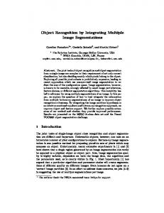
2 Basics of Graph Theory In 1736, Leonard Euler was puzzled whether it is possible to walk across all the bridges on the river Pregel in Königsberg1 only once and return to the starting point (see Fig. 1a). In order to solve this problem, Euler in an ingenious way, abstracted the bridges and the landmasses. He replaced each landmass by a dot (called vertex) and each bridge by an arch (called edge or line) (Fig. 1b). Euler proved that there is no solution to this problem. The Königsberg bridge problem was the first problem studied in what is nowadays called graph theory. This problem was a starting point also for another branch in mathematics, the topology. The definitions given below are compiled from the books [8, 49, 17], therefore the citations are not repeated. The interested reader can find all these definitions and more in the above mentioned literature. Formally, one can define graph G on sets V and E as: 1

Nowadays Pregoyla in Kaliningrad.

Multiresolution Image Segmentations in Graph Pyramids

3

Definition 1 (Graph). A graph G = (V (G), E(G), ιG (·)) is a pair of sets V (G) and E(G) and an incidence relation ιG (·) that maps pairs of elements of V (G) (not necessarily distinct) to elements of E(G). The elements vi of the set V (G) are called vertices (or nodes, or points) of the graph G, and the elements ej of E(G) are its edges (or lines). Let an example be used to clarify the incidence relations ιG (·). Let the set of vertices of the graph G in Fig. 1b) be given by V (G) = {vA , vB , vC , vD } and the edge set by E(G) = {ea , eb , ec , ed , ef , eg }. The incidence relation is defined as : ιG (ea ) = (vA , vB ), ιG (eb ) = (vA , vB ), ιG (ec ) = (vA , vC ), ιG (ed ) = (vA , vC ), ιG (ee ) = (vA , vD ), ιG (ef ) = (vB , vD ), ιG (eg ) = (vC , vD ).

(1)

For the sake of simplicity of the notation, the incidence relation will be omitted, therefore one can write, without the fear of confusion: ea = (vA , vB ), eb = (vA , vB ), ec = (vA , vC ), ed = (vA , vC ), ee = (vA , vD ), ef = (vB , vD ), eg = (vC , vD ).

(2)

i.e. the graph is defined as G = (V, E) without explicit mentioning of the incidence relation. The vertex set V (G) and the edge set E(G) are simply written as V and E. There will be no distinction between a graph and its sets, one may write a vertex v ∈ G or v ∈ V instead of v ∈ V (G), an edge e ∈ G or e ∈ E, and so on. Vertices and edges are usually represented with symbols like v1 , v2 , ... and e1 , e2 , ..., respectively. Note that in Eq. 2, each edge is identified with a pair of vertices. If the edges are represented with ordered pairs of vertices, then the graph G is called directed or oriented, otherwise if the pairs are not ordered, it is called undirected or non-oriented. Two vertices connected by an edge ek = (vi , vj ) are called end vertices or ends of ek . In the directed graph the vertex vi is called the source, and vj the target vertex of edge ek . The elements of the edge set E are distinct i.e. more than one edge can join the same vertices. Edges having the same end vertices are called parallel edges2 . If ek = (vi , vi ), i.e. the end vertices are the same, then ek is called a self-loop. A graph G containing parallel edges and/or self-loops is a multigraph. A graph having no parallel edges and self-loops is called a simple graph. The number of vertices in G is called its order, written as |V |; its number of edges is given as |E|. A graph of order 0 is called an empty graph3, and of order 1 is simply called trivial graph4. A graph is finite or infinite based on its order. If not otherwise stated all the graphs used in this chapter are finite and not empty. Two vertices vi and vj are neighbors or adjacent if they are the end vertices of the same edge ek = (vi , vj ). Two edges ei and ej are adjacent if they have an end vertex in common, say vk , i.e. ei = (vk , vl ) and ej = (vk , vm ). If all vertices of G are pairwise neighbors, then G is complete. A complete graph on m vertices is written as K m . An edge is called incident on its end vertices. The degree (or valency) deg(v) of a vertex v is the number of edges incident on it. A vertex of degree 0 is called isolated; of degree 1 is called pendant. Note that a self-loop at a vertex v contributes twice in deg(v). Let G = (V, E) and G = (V , E ) be two graphs. G = (V , E ) is a subgraph of G (G ⊆ G) if V ⊆ V and E ⊆ E, i.e. the graph G contains graph G . Graph G is called also a supergraph of G (G ⊇ G ). If either V ⊂ V or E ⊂ E, the graph G is called a proper subgraph of G. If G ⊆ G and G contains all the edges e = (vi , vj ) ∈ E such that vi , vj ∈ V , G is the (vertex) induced subgraph of G and V induces (spans) G in G. It is written as G = G[V ], i.e. since V ⊂ G(V ), then G[V ] denotes the graph on V whose edges are the edges of G with both ends in V . If not otherwise stated, by induced subgraph, the vertex-induced subgraph is meant. If there are no isolated vertices in G , then G is called the induced subgraph of G on the edge set E or simply edge induced subgraph of G. If G ⊆ G and V spans all of G, i.e V = V then G is a spanning subgraph of G. A subgraph G of a graph G is a maximal (minimal) subgraph of G with respect to some property Π if G has the property Π and G is not a proper subgraph of any other subgraph of G having the property Π. The minimal and maximal subsets with respect to some property are defined analogously. This definition will be used later to define a component of G as a maximal connected subgraph of G, and a spanning tree of a connected G is a minimal connected spanning subgraph of G. 2 3 4

Also called double edges. A graph with no vertices and hence no edges. A graph with one vertex and possibly with self-loops.

4

Walter G. Kropatsch, Yll Haxhimusa and Adrian Ion

Let G = (V, E) be a graph with sets V = {v1 , v2 , · · · } and E = {e1 , e2 , · · · }. A walk in a graph G is a finite non-empty alternating sequence v0 , e1 , v1 , · · · , vk−1 , ek , vk of vertices and edges in G such that ei = (vi , vi+1 ) for all 1 ≤ i ≤ k. This walk is called a v0 − vk walk with v0 and vk as the terminal vertices and all other vertices are internal vertices of this walk. In a walk, edges and vertices can appear more than once. If v0 = vk , the walk is closed, otherwise it is open. A walk is a trail if all its edges are distinct. A trail is closed if its end vertices are the same, otherwise it is opened. By definition the walk can contain the same vertex many times. A path P is a trail where all vertices are distinct. A simple path is written as P = v0 , v1 , v2 , · · · , vk , where edges are not explicitly depicted since in a path all vertices are distinct and therefore in a simple graph all the edges are distinct too. Note that in a multigraph a path is not uniquely defined by this nomenclature, because of possible multiple edges between two vertices. Vertices v0 and vk are linked by the path P , also P is called a path from v0 to vk (as well as between v0 and vk ). The number of edges in the path is called the path length. The path length is denoted with P k , where k is the number of edges in the path. Note that by definition it is not necessary that a path contains all the vertices of the graph. Cycles, like paths, are denoted by the cyclic sequence of vertices C = v0 , v1 , · · · , vk , v0 . The length of the cycle is the number of edges in it is called k-cycle written as C k . The minimum length of a cycle in a graph G is the girth g(G) of G, and the maximum length of a cycle is its circumference. The distance between two vertices v and w in G denoted by d(u, w), is the length of the shortest path between these vertices. The diameter of G, diam(G) is the maximum distance between any two vertices of G. Connectivity is an important concept in graph theory and it is one of the basic concepts used in this presentation. Two vertices vi and vj are connected in a graph G = (V, E) if there is a path vi − vj in G. A vertex is connected to itself. A non-empty graph is connected if any two vertices are joint by a path in G. Let graph G = (V, E) be a non-connected graph. The set V is partitioned into subsets V1 , V2 , · · · , Vp if V1 ∪ V2 ∪ · · · ∪ Vp = V and for all i and j, i = j Vi ∩ Vj = ∅. {V1 , V2 , · · · , Vp } is called a partition of V . Since the graph G is non-connected, the vertex set V can be partitioned into subsets V1 , V2 , · · · , Vp , such that each vertex induced subgraph G[Vi ] is connected, and there exists no path between a vertex in subset Vi and a vertex in Vj , j = i. A maximally connected subgraph of G is called a component of graph G. A component of G is not a proper subgraph of any other connected subgraph of G. An isolated vertex is considered to be a component, since by definition it is connected to itself. Note that a component is always non-empty, and that if a graph G is connected then it has only one component, i.e. itself. The following theorem is used in the Sec. 5 to show that after the edge removal from the cycle the graph stays connected. Theorem 1. If a graph G = (V, E) is connected, then the graph remains connected after the removal of an edge e of a cycle C ∈ E, i.e. G = (V, E − {e}) is connected. Proof. The proof can be found in [8]. From the above theorem one can conclude that edges that if removed disconnect a graph, do not lie on any cycle. The definition of cut and cut-set are as follows. Let {V1 , V2 } be partitions of the vertex set V of a graph G = (V, E). The set K(V1 , V2 ) of all edges having one end in one vertex partition (V1 ) and the other end on the second vertex partition (V2 ) is called a cut. A cut-set KS of a connected graph G is a minimal set of edges such that its removal from G disconnects G, i.e. G − KS is disconnected. If the induced subgraphs of G on vertex set V1 and V2 are connected then K = KS . If the vertex set V1 = {v}, the cut is denoted by K(v). Trees are simple graph structures, and are extensively used in the rest of the discussion. A graph G is acyclic if it has no cycles. A tree of graph G is a connected acyclic subgraph of G. Vertices of degree 1 in a tree are called leaves, and all edges are called branches. A non-trivial tree has at least two leaves and a branch, for example the simplest tree consists of two vertices joined by an edge. Note that an isolated vertex is by definition an acyclic connected graph, and therefore a tree. A spanning tree of graph G is a tree of G containing all the vertices of G. Edges of the spanning tree are called branches. The tree containing all vertices, and only those edges not in the spanning tree, is called cospanning tree, and its edges are called cords. An acyclic graph with k components is called a k-tree. If the k-tree is a spanning subgraph of G, then it is called a spanning k-tree of G. A forest F of a graph G is a spanning k-tree of G, where k is the number of component of G. A forest is simply a set of trees, spanning


5

G vj e vi

vk

vj vj

vi

vk

v∗

vk a) vertex vi removal

ek

b) edge e removal

vk

c) identifying vi with vj

v∗

vk

d) contracting edge e

Figure 2. Operations on graph.

all the vertices of G. A connected subgraph of a tree T is called a subtree of T . If T is a tree then there is exactly one unique path between any two vertices of T . And finally some basic binary and unary operations on graphs are described. Let G = (V, E) and G = (V , E ) be two graphs. Three basic binary operations on two graphs are as follows: Union and Intersection. The union of G and G is the graph G = G ∪ G = (V ∪ V , E ∪ E ), i.e. the vertex set of G is the union of V and V , and the edge set is the union of E and E , respectively. The intersection of G and G is the graph G = G ∩ G = (V ∩ V , E ∩ E ), i.e. the vertex set of G has only those vertices present in both V and V , and the edge set contains only those edges present in both E and E , respectively. Symmetric Difference. The symmetric difference5 between two graphs G and G , written as G ⊕ G , is the induced graph G on the edge set E E = (E \ E ) ∪ (E \ E)6 , i.e. this graph has no isolated vertices and contains edges present either in G or in G but not in both. Four unary operations on a graph are as follows: Vertex Removal. Let vi ∈ G, then G − vi is the induced subgraph of G on the vertex set V − vi ; i.e. G − vi is the graph obtained after removing the vertex vi and all the edges ej = (vi , vj ) incident on vi . The removal of a set of vertices from a graph is done as the removal of single vertex in succession. An example of vertex removal is shown in Fig. 2a). Edge Removal. Let e ∈ G, then G − e is the subgraph of G obtained after removing the edge e from E. The end vertices of the edge e = (vi , vj ) are not removed. The removal of a set of edges from a graph is done as the removal of single edge in succession. An example of edge removal is shown in Fig. 2b). Vertex Identifying. Let vi and vj be two distinct vertices of graph G joined by the edge e = (vi , vj ). Two vertices vi and vj are identified if they are replaced by a new vertex v ∗ such that all the edges incident on vi and vj are now incident on the new vertex v ∗ . An example of vertex identifying is given in Fig. 2c). Edge Contraction. Let e = (vi , vj ) ∈ G be the edge with distinct end points vi = vj to be contracted. The operation of edge contraction denotes removal of the edge e and identifying its end vertices vi and vj into a new vertex v ∗ . If the graph G results from G after contracting a sequence of edges, than G is said to be contractible to a graph G . Note the difference between vertex identifying and edge contraction, in Fig. 2c) and d). Vertex identifying preserves the edge ek , whereas edge contraction first removes this edge. In Sec. 5 a detailed treatment of edge contraction and edge removal in the dual graphs context is presented.

5 6

Called also ring sum. Where \ is the set minus operation and is interpreted as removing elements from X that are in Y .

6

Walter G. Kropatsch, Yll Haxhimusa and Adrian Ion 1 λ

h

λ2 1 level 0

λn s a) Pyramid concept

reduction window b) Discrete levels

Figure 3. Multiresolution pyramid.

3 Image Pyramids Visual data is characterized by large amount of data and high redundancy with relevant information clustered in space and time. All this indicates a need of organization and aggregation principles, in order to cope with computational complexity and to bridge the gap between raw data and symbolic description. Local processing is important in early vision, since operations like convolution, thresholding, mathematical morphology etc. belong to this class. However, using them is not efficient for high or intermediate level vision, such as symbolic manipulation, feature extraction etc., because these processes need both local and global information. Therefore a data structure must allow the transformation of local information (based on sub-images) into global information (based on the whole image), and be able to handle both local (distributed) and global (centralized) information. Such a data structure, the pyramid, is known as hierarchical architecture [26], and it allows distribution of the global information to be used by local processes. The pyramid is a trade off between parallel architecture and the need for a hierarchical representation of an image, i.e. at several resolutions [26]. An image pyramid (Fig. 3a,b) describes the contents of an image at multiple levels of resolution. High resolution input image is at the base level. Successive levels reduce the size of the data by a reduction factor λ > 1.0. Reduction windows relate one cell at the reduced level with a set of cells in the level directly below. Thus, local independent (and parallel) processes propagate information up and down and laterally in the pyramid. The contents of a lower resolution cell are computed by means of a reduction function the input of which are the descriptions of the cells in the reduction window. Sometimes the description of the lower resolution needs to be extrapolated to the higher resolution. This function is called the refinement or expansion function. It is used in Laplacian pyramids [5] and wavelets [39] to identify redundant information in the higher resolution and to reconstruct the original data. Two successive levels of a pyramid are related by the reduction window and the reduction factor. Higher level description should be related to the original input data in the base of the pyramid. This is identified by the receptive field (RF) of a given pyramidal cell ci . The RF (ci ) aggregates all cells (pixels) in the base level of which ci is the ancestor. Based on how the cells in subsequent levels are joint, two types of pyramids exist: • •

regular, and irregular pyramids.

These concepts are strongly related to the ability of the pyramid to represent the regular and irregular tessellation of the image plane. Regular Pyramids The constant reduction factor and constant size reduction window completely define the structure of the regular pyramid. The decrease rate of cells from level to level is determined by the reduction factor. The number of levels h is limited by the reduction factor λ > 1.0: h ≤ log(image size)/ log(λ). The main computational advantage of regular image pyramids is due to their logarithmic complexity. Usually regular pyramids are employed in a regular grid tessellated image plane, therefore the reduction window is usually a square of n×n, i.e. the n×n cells are associated to a cell on a higher level directly above. Regular pyramids


7

are denoted using notation n × n/λ. The vertical structure of a classical 2 × 2/4 is given in Fig. 4a). In this regular pyramid 2 × 2 = 4 cells are related to only one cell in the level directly above. Since the children have only one parent this class of pyramids is also called non-overlapping regular pyramids. Therefore the reduction factor is λ = 4. An example of 2 × 2/4 regular image pyramid is given in Fig. 4b). The image size is 512 × 512 = 29 × 29 therefore the image pyramid consist of 1 + 2 · 2 + 4 · 4 + ... + 28 × 28 + 29 × 29 cells, and the height of this pyramid is 9. The pyramid levels are shown by a white border on the left upper corner of image. See [30] for extensive overview of other pyramid structures with overlapping reduction windows, e.g. 3 × 3/2, 5 × 5/4. It is possible to define pyramids on other plane tessellation, e.g. triangular tessellation [26]. Thus, because of the rigid vertical structure, the regular image pyramid is an efficient structure for fast grouping and access to image objects across the input image, The regular pyramid representation of a shifted, rotated and/or scaled image is not unique, and moreover it does not preserve the connectivity. Thus, [3] concludes that regular image pyramids have to be rejected as general-purpose segmentation algorithms. This major drawback of the regular pyramid motivated a search for a structure that is able to adapt on the image data. It means, that the regularity of the structure is to be abandoned. Irregular Pyramids Abandoning the regularity of the structure means that the horizontal and vertical neighborhood have to be explicitly represented, usually by using graph formalisms. These irregular structures are usually called irregular pyramids. One of the main goals of irregular pyramids is to achieve the shift invariance, and to overcome this major drawback of their regular counterparts. Other motivations why one has to use irregular structures are [36]: arrangement of biological vision sensors is not completely regular; the CCD cameras cannot be produced without failure, resulting in an irregular sensor geometry; perturbation may destroy the regularity of regular pyramids; and image processing to arbitrary pixels arrangement (e.g. log-polar geometries [1]). Two main processing characteristics of the regular pyramids should be preserved by building irregular ones [2]: (i) operation are local, i.e. the result is computed independently of the order, this allows parallelization, and (ii) bottom-up building of the irregular pyramid, with an exponential decimation of the number of cells. The structure of the regular pyramid as well as the reduction process is determined by the type of the pyramid (e.g. 2 × 2/4). After removing this regularity constraint one has to define a procedure to derive the structure of the reduced graph Gk+1 from Gk , i.e. a graph contraction method has to be defined. Irregular pyramids can be build by parallel graph contraction [45], or graph decimation [41]. Parallel graph contraction has been developed only for special graph structures, like trees, and is not discussed in this chapter. The graph decimation procedure is described in Sec. 5. An efficient random decimation algorithm for building regular pyramids, called stochastic pyramids (MIS) is introduced in [41]. A detailed discussion of this and similar methods is done in [35]. It is shown that MIS in some cases is not logarithmically tapered, i.e. the decimation process does not successively reduce the number of cells exponentially. The main reason for this behavior is that the cell’s neighborhood is not bounded, for some cases the degree of

a) vertical structure

b) image pyramid

Figure 4. 2 × 2/4 regular pyramid.

8


the cell increases exponentially. In [35], two new methods based on maximal independent edge set (MIES and MIDES) that overcome this drawback are presented. An overview of the properties of regular and irregular pyramids is found in [37]. In irregular pyramids the flexibility is paid by less efficient data access. Most information in vision today is in the form of array representation. This is advantageous and easily manageable for situations having the same resolution, size, and other typical properties equivalent. Various demands are appearing upon more flexibility and performance, which makes the use of array representations less attractive [15]. The increasing use of actively controlled and multiple sensors requires a more flexible processing and representation structure [36, 34]. Cheaper CCD sensors could be produced if defective pixels would be allowed, which yields in the resulting irregular sensor geometry [1, 50]. Image processing functions should be generalized to arbitrary pixel geometries [44, 1]. The conventional array form of images is impractical as it has to be searched and processed every time if some action is to be performed and (i) features of interest may be very sparse over parts of an array, leaving a large number of unused positions in the array; (ii) a description of additional detail can not be easily added to a particular part of an array. In order to express the connectivity or other geometric or topological properties, the image representation must be enhanced by a neighborhood relation. In the regular square grid arrangement of sampling points, it is implicitly encoded as 4- or 8-neighborhood with the well known paradox in conjunction with Jordan’s curve theorem. The neighborhood of sampling points can be represented explicitly, too: in this case the sampling grid is represented by a graph consisting of vertices corresponding to the sampling points and of edges connecting neighboring vertices. Although this data structure consumes more memory space it has several advantages, as follows [36]: the sampling points need not be arranged in a regular grid; the edges can receive additional attributes too; and the edges may be determined either automatically or depending on the data. In irregular pyramids, each level represents a partition of the pixel set into cells, i.e. connected subsets of pixels. The construction of an irregular image pyramid is iteratively local [41, 19]: • • •

the cells have no information about their global position, the cells are connected only to (direct) neighbors, and the cells cannot distinguish the spatial positions of the neighbors.

This means that we use only local properties to build the hierarchy of the pyramid. Usually, on the base level (level 0) of an irregular image pyramid the cells represent single pixels and the neighborhood of the cells is defined by the 4 -connectivity of the pixels. A cell on level k + 1 (parent) is a union of neighboring cells on level k (children). As shown in Sec. 5 this union is controlled by contraction kernels (decimation parameters). Every parent computes its values independently of other cells on the same level. This implies that an image pyramid is built in O[log(image diameter)] parallel steps. Neighborhoods on level k + 1 are derived from neighborhoods on level k. Two cells c1 and c2 are neighbors if there exist pixels p1 in c1 and p2 in c2 such that p1 and p2 are 4-neighbors. Before we continue with the presentation of graph pyramids, a concept of planar graphs is needed. A planar graph separates the plane into regions called faces. This idea of separating the plane into regions is helpful in defining the dual graphs. Duality of a graph brings together two important concepts in graph theory: cycles and cut-sets. This concept of duality is also encountered in the graph-theoretical approach of image region and edge extraction. The definition of dual graphs representing the partitioning of the plane, allows one to apply transformations on these graphs, like edge contraction and/or removal to simplify them in the sense of less vertices and edges. Edge contraction and removal introduces naturally a hierarchy of dual graphs, the so called dual graph pyramid.

4 Planar and Dual Graphs of finite sets of vertices V and edges E is called plane graph if it can be drawn in a plane in R2 A graph G such that [8]: •

all V ⊂ R2

Multiresolution Image Segmentations in Graph Pyramids G = (V, E)

9

f4

e6 e4

v2 e5

e1

f3

v4 e3

e7

e9 v5 e8

v1

e2

f5 f2

f1 e5

b G

v3 Figure 5. A planar graph G and its embedding in a plane, the plane graph G.

• •

every edge is an arc7 between two vertices, no two edges are crossed.

is an open set and its connected regions are faces f of G. It is said that the plane graph Note that R \ G divides the plane into regions. Since G is bordered, one of its faces is an unbounded one (infinite area). This face is called the background face8 . The other faces enclose finite areas, and are called interior faces. Edges and vertices incident to a face are called the boundary elements of that face. A planar embedding of G is called a drawing of G. Similar to G, G a graph G is an isomorphism between G and a plane graph G. is drawn so that its edges intersect only on vertices. A graph G is planar if it can be embedded on the plane. The concept of embeddings can be extended to any surface. A graph G is embeddable in surface S if it can be drawn in S so that its edges intersect only on their end vertices. A graph embeddable on the plane is embeddable on the sphere too. It can be shown by using the stereoscopic projection of the sphere onto a plane [49]. Note that the concept of faces is also applicable to spherical embeddings. Let G in Fig. 5 represent a planar graph, in general with parallel edges and self-loops. Since the graph is embedded onto a plane, it divides the plane into faces. Let each of these faces be denoted by a new vertex say f , and let these vertices be put inside the faces, as shown in Fig. 5 From this point on the notion of face vertices and face are synonymous. Let the faces that are neighbors, i.e. that share the same edge e2 (they are incident on the same edge), be connected by the edge, say e2 , so that edges e2 and e2 are crossed. At the end, for each edge e2 ∈ G there is an edge e2 of the newly created graph G, which is called the dual graph of G. If e2 is incident only with one face a self-loop edge e2 is attached to the vertex on the face in which the edge e2 lays, of course e2 and the self-loop edge e2 have to cross each other. The adjacency of faces is expressed by the graph G. More formally one can define dual graphs for a given plane graph G = (V, E) [49]: Definition 2 (Dual graphs). A graph G = (V , E) is a dual of G = (V, E) if there is a bijection between the edges of G and G, such that a set of edges in G is a cycle vector if and only if the corresponding set of edges in G is a cut vector. There is a one-to-one correspondence between the vertex set V of G and the face set F of G, therefore sometimes graph G = (V , E) is written as G = (F, E) instead, without fear of confusion. In order to show that G is a dual of G, one has to prove that vectors forming a basis of the cycle subspace of G correspond to the vectors forming a basis of the cut subspace of G. The edges ei of graph G in Fig. 6 correspond to edges ei in graph G. The cycles {e1 , e3 , e4 }, {e2 , e3 , e6 }, {e4 , e5 , e8 }, and {e6 , e7 , e8 } form a basis of the cycle subspace of G. These cycles correspond to the set of edges {e1 , e3 , e4 }, {e2 , e3 , e6 }, {e4 , e5 , e8 }, and {e6 , e7 , e8 }, which form a basis of the cut subspace of G. It follows according to the definition of the duality, that graph G is a dual of G. The graph G is called the primal graph and G the dual graph. Dual 7 8

An arc is a finite union of straight line segments, and a straight line segment in the Euclidean plane is a subset of R2 of the form {x + λ(y − x)|0 ≤ λ ≤ 1}∀ x = y ∈ R2 . Called also exterior face.

10


G = (V, E) e2

e2

G = (F, E)

e5 e4

v2

e4 v3

v4

v4

e8

e3 e3

e1

e6

e8 v5

e1

v5 e6

v2 e2

e5

e7 v1

e2

e7

v3

v1 Figure 6. A plane graph G and it dual G.

graphs are denoted by a line above the big letter. If a planar graph G is a dual of G, then a planar G is a dual of G as well, and every planar graph has a dual [8, 17] . In the following, two important properties of dual graphs with respect to the edge contraction and removal operations are given, the proofs are due to [49]. These properties are required to prove that during the process of dual graph contraction graphs stay planar and are duals (Sec. 5). Let G and its dual G be two graphs. Let edge e ∈ G correspond to edge e ∈ G. Note that a cycle in G corresponds to a cut in G and vice versa [49]. Let G denote the graph G after the contraction of the edge e, and G the graph after the removal of the corresponding edge e from G. Theorem 2. A graph and its dual are duals also after the removal of an edge e in the primal graph G and the contraction of the corresponding edge e in the dual graph G. Corollary 1. If a graph G has a dual, then every edge-induced subgraph of G has also a dual. Theorem 3 (Whitney 1933). A graph is planar if and only if it has a dual. Proof. The proofs can be found in [49] and [8]. Dual Image Graphs An image is transformed into a graph such that, to each pixel a vertex is associated, and pixels that are neighbors in the sampling grid are joint by an edge. Note that no restriction on the sampling grid is made, therefore an image of regular as well as non-regular sampling grid can be transformed into a graph. The gray value or any other feature is simply considered as an attribute of a vertex (and/or an edge). Since the image is finite and connected, the graph is finite and connected as well. The graph which represents the pixels is denoted by G = (V, E) and is called primal graph9 . Note that pixels represent finite regions, and the graph G is representing in fact a graph with faces as vertices. The dual of a face graph (see Sec. 4) is the graph representing borders of the faces, which in fact are inter-pixel edges and inter-pixel vertices. This graph is denoted by G and is called simply dual graph. Based on Theorem 3, dual graphs are planar, therefore images with square grid are transformed into 4− connected square grid graphs, since 8− connected square grid graphs are in general not planar 10 . The same formalism as done for the pixels can be used at intermediate levels in image analysis i.e. for region adjacency graphs (RAGs). RAGs can be the results of image segmentation processes. Regions 9 10

Also called neighborhood graph. This holds for square grid graphs of grid size ≥ 4 × 4.


Image

Primal graph G Figure 7. Image to dual graphs.

11

Dual graph G

are connected sets of pixels, and are separated by region borders. Their geometric dual though causes problems [32]. This section is concluded by a formal definition of the dual image graphs: Definition 3 (Dual image graphs [31]). The pair of graphs (G, G), where G = (V, E) and G = (V , E) are called dual image graphs if both graphs (G, G) are finite, planar, connected, not simple in general and duals of each other. Dual graphs can be seen as an extension of the well know region adjacency graphs (RAG) representation. Note that this representation is capable to encode not only adjacency relations but inclusion relations as well [32].

5 Dual Graph Contraction Irregular (dual graph) pyramids are constructed in a bottom-up way such that a subsequent level (say k + 1) results by (dually) contracting the precedent level (say k). In this section a short exposition of the dual graph contraction is given, following the work of Kropatsch [32]. Building dual graph pyramids using this algorithm is presented in the next section. Dual graph contraction (DGC) [32] proceeds in two steps: I. primal-edge contraction and removal of its dual, and II. dual-edge contraction and removal of its primal. In Fig. 8 examples of these two steps are shown in three possible cases. Note that these two steps correspond in [32] to the steps (I) dual edge contraction, and (II) dual face contraction. The base of the pyramid consists of the pair of dual image graphs (G0 , G0 ). In order to proceed with the dual graph contraction a set of so called contraction kernels (decimation parameters) must be defined. The formal definition is postponed until the Sec. 5. Let the set of contraction kernels be Sk , Nk,k+1 . This set consists of a subset of surviving vertices Sk = Vk+1 ⊂ Vk , and a subset of non-surviving primal-edges Nk,k+1 ⊂ Ek (where index k, k + 1 refer to contraction from level k to k + 1). Surviving vertices in v ∈ Sk are vertices not to be touched by the contraction, i.e. after contraction these vertices make up the set Vk+1 of the graph Gk+1 ; and every non-surviving vertex v ∈ Vk \Sk must be paired to one surviving vertex in a unique way, by non-surviving primal-edges (Fig. 9a). In this figure, the shadowed vertex s is the survivor and this vertex is connected with arrow edges (ns) with non-surviving vertices. Note that a contraction kernel is a tree of depth one, i.e. there is only one edge between a survivor and a non-survivor, or analogously one can say that the diameter of this tree is two. The contraction of a non-surviving primal-edge consists in the identification of its endpoints (vertices) and the removal of both the contracted primal-edge and its dual edge (see Sec. 2 for details on these operations). Fig. 10a) shows the normal situation, Fig. 10b) the situation where the primal-edge contraction creates multiple edges, and Fig. 10c) self-loops. In Fig. 10c), redundancies (lower part) are decided through the corresponding dual graphs and removed by dual graph contraction. In Fig. 10, the primal graph is shown with square () vertices and broken lines (- -) and its dual with circle vertices (P) and full lines (-). In [32] it is shown that Sk , Nk,k+1 determine the structure of an irregular pyramid. The relation between two pairs of dual graphs,(Gk , Gk ) and (Gk+1 , Gk+1 ), is established by dual graph contraction with the set of contraction kernels Sk , Nk,k+1 as:

12

Walter G. Kropatsch, Yll Haxhimusa and Adrian Ion Pair of dual graphs (Gk , Gk ) at level k of the pyramid primal graph dual graph Gk = (Vk , Ek )

duals

G = (Sk , Ek \ Nk,k+1 )

duals

Gk+1 = (Vk+1 , Ek+1 )

duals

↔ Gk = (V k , E k ) ⇓ I. Primal-edge contraction and removal of its dual primal-edge contraction in Gk and corresponding dual-edge removal in Gk ↓ ↓ ↔ G = (V k , E k \ N k,k+1 ) ⇓ II. Dual-edge contraction and removal of its primal Remove all v with deg(v) ≤ 2 primal-edge removal in G and corresponding dual-edge contraction in G ↓ ↓ ↔ Gk+1 = (V k+1 , E k+1 ) ⇓ Pair of dual graphs (Gk+1 , Gk+1 ) at level k + 1 of the pyramid Figure 8. Dual graph contraction procedure (DGC).

(Gk+1 , Gk+1 ) = C[(Gk , Gk ), Sk , Nk,k+1 ].

(3)

Dual-edge contraction and removal of its primal (second step) has a role of cleaning the primal graph by simplifying most of the multiple edges and self-loops11, but not those enclosing any surviving parts of the graph. They are necessary to preserve correct structure [32]. Dual graph contraction reduces the number of vertices and edges of a pair of dual graphs, while preserving the topological relations among surviving parts of the graph. In [31, 33] a detailed presentation of dual graph contraction is given. Contraction Kernels Let S be the set of surviving vertices, and N the set of non-surviving primal-edges. The connected components 12 CC(s), s ∈ S, of subgraph (S, N ) form a set of rooted tree structures T (s) that, if contracted, a)

b) k+1

n1

v

s n2 tree of depth one

n4

k

s

n3

contraction kernel

s ∈ Vk and v ∈ Vk+1 s ∈ Sk and n1 , n2 , n3 , n4 ∈ Nk,k+1 Creation of a new vertex v in the level k + 1 of the pyramid

Figure 9. a) Contraction kernel and b) parent-child relation. 11 12

Called also redundant edges. Neglected level indexes refer to contraction from level k to level k + 1.

Multiresolution Image Segmentations in Graph Pyramids a) normal case

b) multiple edges

13

c) self loops

⇓

⇓ ⇓ I. Primal-edge contraction and removal of its dual ⇓ ⇓ ⇓

vi

deg(v) > 2, ∀v

vi

deg(vi ) ≤ 2 ⇓ ⇓ II. Dual-edge contraction and removal of its primal ⇓ ⇓

Figure 10. Dual graph contraction of a part of a graph.

each of them would collapse into the vertex s of the contracted graph. The number of these trees is |S|. The union of trees T (s) contains the non-surviving primal-edges N . T (s) is a spanning tree of the connected component CC(s), or equivalently, (V, N ) is a spanning forest of the graph G = (V, E). In order to decimate the graph G = (V, E) the set of surviving vertices S ⊂ V and the set of non-surviving primal-edges N ⊂ E must be selected, such that the following conditions are satisfied: (1) graph (V, N ) is a spanning forest of graph G = (V, E), and (2) the surviving vertices s ∈ S ⊂ V are the roots of the forest (V, N ). Definition 4 (Contraction kernels). A set of disjoint rooted trees with length two of path going through the root is called a set of contraction kernels. Analogously, the trees T (v) of the forest (V, N ) with roots v ∈ V are contraction kernels. After applying the dual graph contraction algorithm on a graph, one has to establish a path connecting two surviving vertices on the resulted new graph. Let G = (V, E) be a graph with decimation parameters (S, N ). Definition 5 (Connecting path [31]). A path in G = (V, E) is called a connecting path between two surviving vertices s, s ∈ S if it consists of three subsets of edges: • •

the first part is a possibly empty branch of contraction kernel T (s). the middle part is an edge e ∈ E \ N that bridges the gap between (connects) the two contraction kernels T (s) and T (s ).

14

Walter G. Kropatsch, Yll Haxhimusa and Adrian Ion first part middle part s e

T (s )

T (s) Gk = (Vk , Ek )

second part s CP (s, s )

↓ DGC ↓

Gk+1 = (Vk+1 , Ek+1 ) e = (v, v ) Figure 11. Connecting path CP (v, v ), e is the bridge of this path.

•

the third part is a possibly empty branch of contraction kernel T (s ).

See Fig. 11 for explanation. The connecting path is denoted by CP (s, s ). Edge e is called the bridge of the connecting path CP (s, s ). Each edge e = (v, v ) ∈ Ek+1 has a corresponding connecting path CPk (s, s ), where s, s ∈ S ⊂ Vk are survivors in the graph Gk = (Vk , Ek ). This means that two surviving vertices s and s , s = s , that can be connected by a path13 CPk (s, s ) in Gk are connected by an edge in Ek+1 . If the graph Gk is connected, after dual graph contraction the connectivity of the graph Gk+1 is preserved [31]. Dual edge contraction can be implemented by (1) simply renaming all the non-surviving vertices to their surviving parent vertex (e.g. by using a find union set algorithm [7]), (2) deleting all non-surviving edges N and (3) their duals N . We use different (MIS, MIES, and D3P) stochastic methods to build contraction kernels [35]. Equivalent contraction kernels [5] combines two or more successive reductions in one equivalent weighting function in order to compute any level of any regular pyramid directly from the base level. Similarly, [33] combines two (or more) dual graph contractions (as shown in Fig. 12) of graph Gk = (Vk , Ek ) with decimation parameters Sk , Nk,k+1 and Sk+1 , Nk+1,k+2 into one single equivalent contraction kernel (ECK) Nk,k+2 = Nk,k+1 ◦ Nk+1,k+2 14 : C[C[Gk , Sk , Nk,k+1 ], Sk+1 , Nk+1,k+2 ] = C[Gk , Sk+1 , Nk,k+2 ] = Gk+2 (4) The structure of Gk+1 is determined by Gk and the decimation parameters Sk , Nk,k+1 . Simply overlaying the two sets of contraction kernels, Sk , Nk,k+1 (the one from level k to k + 1) and Sk+1 , Nk+1,k+2 (the one from level k + 1 to k + 2) will not yield a proper equivalent contraction kernel Sk+1 , Nk,k+2 . The surviving vertices from Gk to Gk+2 are Sk+1 = Vk+2 . The edges of the searched contraction kernels ) ∈ Nk+1,k+2 corresponds to a must be formed by edges Nk,k+2 ⊂ Ek . An edge ek+1 = (vk+1 , vk+1 15 connecting path CPk (vk+1 , vk+1 ) in Gk . By Definition 5, CPk (vk+1 , vk+1 ) consists of one branch of Tk (vk+1 ), one branch of Tk (vk+1 ), and one surviving edge ek ∈ Ek connecting the two contraction kernels Tk (vk+1 ), and Tk (vk+1 ). Definition 6 (Bridge [31]). Function bridge: Ek+1 → Ek assigns to each edge ek+1 = (vk+1 , wk+1 ) ∈ Ek+1 one of the bridges ek ∈ Ek of the connecting paths CPk (vk+1 , wk+1 ): bridge(ek+1 ) = ek . 13 14 15

By definition of the connectivity of a graph, there exists always a path between any two vertices of graph. Only Gk is shown instead of (Gk , Gk ) for simplicity. If there are more than one connecting paths, one is selected.

(5)

Multiresolution Image Segmentations in Graph Pyramids (Gk , Gk ) ↓

DGC

⇒

Sk , Nk,k+1 DGC

(Gk+1 , Gk+1 ) ↓

DGC

15

Sk+1 , Nk,k+2

Sk+1 , Nk+1,k+2

(Gk+2 , Gk+2 ) ⇐ Figure 12. Equivalent contraction kernel.

Connecting two disjoint tree structures by a single edge results in a new tree structure. Now, Nk,k+2 can be defined as the result of connecting all contraction kernels Tk by bridges as: bridge(ek+1 ) (6) Nk,k+2 = Nk,k+1 ∪ ek+1 ∈Nk+1,k+2

This definition satisfies the requirements of a contraction kernel [31]. Analogously, the above process can be repeated for any pair of levels k and k such that k < k . If k = 0 and k = h, where h is the level index of the top of the pyramid, with the resulting equivalent contraction kernel (N0,h ), the base level (0) is contracted in one step into an apex Vh = {vh }. ECKs are able to compute any level of the pyramid directly from the base. Dual Graph Pyramid A graph pyramid is a pyramid where each level is a graph G(V, E) consisting of vertices V and of edges E relating two vertices. In order to correctly represent the embedding of the graph in the image plane [13], we additionally store the dual graph G(V , E) at each level. The levels are represented as pairs (Gk , Gk ) of dual plane graphs Gk and Gk . See Sec. 4 for more details on this representation. The sequence (Gk , Gk ), 0 ≤ k ≤ h is called dual graph pyramid, where 0 is the base level index and h is the top level index, also called the height of the pyramid. Moreover the graphs are attributed, G(V, E, attrv , attre ), where attrv : V → R+ and attre : E → R+ , i.e. content of the graph is stored in attributes attached to both vertices and edges. In general a graph pyramid can be generated bottom-up as shown in Alg. 1. Algorithm 1 – Constructing Dual Graph Pyramid Input: Graphs (G0 , G0 ) 1: k ← 0. 2: while further abstraction is possible do 3: determine contraction kernels, Nk,k+1 . 4: perform dual graph contraction and simplification of dual graphs, (Gk+1 , Gk+1 ) = C[(Gk , Gk ), Nk,k+1 ]. 5: apply reduction functions to compute content attr : Gk+1 → R+ of new reduced level. 6: k ← k + 1. 7: end while Output: Graph pyramid – (Gk , Gk ), 0 ≤ k ≤ h .

Let the building of the dual graph pyramid be explained by using the image in Fig. 7 For the sake of simplicity of the presentation, in the figures afterward, the dual graphs are not shown explicitly as well as intra-level relations. An example of this intra-level relation is shown in Fig. 9b) with the contraction kernel shadowed. In the example from Fig. 13 initially the attributes of the vertices receive the gray values of the pixels. The first step determines what information in the current top level is important and what

16


a) image to graph G0

b) contraction kernel N01

double edges

c) G after dual-edge contraction of G0 d) G1 after the removal of redundant edges in G Figure 13. Dual graph contraction in G0 and the creation of the G1 of the pyramid.

can be dropped. A contraction kernel is a (small) sub-tree of the top level, the root of which is chosen to survive (black circles in Fig. 13b). Fig. 13a) shows the window and the selected contraction kernels with gray. Selection criteria in this case contracts only edges inside connected components having the same gray value. All the edges of the contraction trees are dually contracted during step 3 from Alg. 1. Dual contraction of an edge e (formally denoted by G/{e}) consists of contracting e and removing the corresponding dual edge e from the dual graph (formally denoted by G \ {e}). This preserves duality and the dual graph needs not be constructed from the contracted primal graph G at the next level. Since the contraction of an edge may yield multi-edges (an example shown with arrows in Fig. 13c) and self-loops there is a second simplification phase of step 3 which removes all redundant multi-edges and self-loops. Note that not all such edges can be removed without destroying the topology of the graph: if the cycle formed by the multi-edge or the self-loop surrounds another part of the data its removal would corrupt the connectivity! Fortunately this can be decided locally by the dual graph since faces of degree two (having the double-edge as boundary) and faces of degree one (boundary = self-loop) cannot contain any connected elements in its interior. Since removal and contraction are dual operations, the removal of a self-loop or of one of the double edges can be done by contracting the corresponding dual edges in the dual graph (which are not depicted in our example for the sake of simplicity). The dual contraction from our example remains a simple graph G1 without self-loops and multi-edges (Fig. 13d). Step 3 generates a reduced pair of dual graphs. Their contents is derived in step 4 from the level below using the reduction function. In our example reduction is very simple: the surviving vertex inherits the color of its sons. The following table summarizes dual graph contraction in terms of the control parameters used for abstraction and the conditions to preserve topology: level 0

1

representation contract / remove (G0 , G0 ) ↓ contraction kernel N0,1 (G0 /N0,1 , G0 \ N0,1 ) ↓ redundant edges S0,1 (G1 = G0 /N0,1 \ S0,1 , G1 = G0 \ N0,1 /S0,1 ) ↓ contraction kernel N1,2 .. .

conditions forest, depth 1 deg v ≤ 2 forest, depth 1

6 A Hierarchy of Partitions The segmentation problem is supposed to find natural groupings of the pixel set given as input. The first question that comes in mind is how these natural groupings are found. In other words what makes pixels in


17

Algorithm 2 – Boruvka’s ˚ Algorithm Input: graph G(V, E) 1: M ST ← empty edge list 2: all vertices v ∈ V make a list of trees L 3: while there is more than one tree in L do 4: each tree T ∈ L finds the edge e with the minimum weight which connects T to G \ T and add edge e to MST. 5: using edge e merge pairs of trees in L 6: clean the graph from self-loops if necessary 7: end while Output: minimum weight spanning tree - edge induced subgraph on MST.

a partition be more like one another than pixels in other segments. This observation pours down into two issues [9]: (i) how to measure the similarity between pixels, and (ii) how to evaluate a partitioning of the pixels into segments. It is expected that, these measures of dissimilarity capture the expectation that the distance in a feature space of pixels within a segment is less than the distance between pixels in different segments. The second issue is defining the criterion function to be optimized. The goal is to find the groups or segments that have strong internal similarities, which optimize the criterion function. But before we continue with the presentation of the algorithm for hierarchical image partitioning, let we recall the idea of minimum spanning tree (MST) and Bor˚uvka’s algorithm. Minimum Weight Spanning Tree (MST) The minimum spanning tree, called afterward MST, is the simplest and best-studied optimization problem in computer science. According to [42] the ”Minimum spanning tree is a cornerstone problem of combinatorial optimization and in a sense its cradle”. The problem is defined as follows. Let G = (V, E) be a undirected connected plane graph consisting of the finite set of vertices V and the finite set of edges E. Each edge e ∈ E is identified with a pair of vertices vi , vj ∈ V such that vi = vj . Let each edge e ∈ E be associated with a unique weight w(e) = w(vi , vj ), from the totally ordered universe (it is assumed that weights are distinct, if not, ties can be broken arbitrarily). Note that parallel edges, for e.g. e1 = (v1 , v2 ) and e2 = (v1 , v2 ) e1 = e2 , have different weights. The problem is formulated as construction of a minimum total weight spanning tree of G. Boruvka’s ˚ Algorithm The idea of Bor˚uvka [4] is to do steps like in Prim’s algorithm [43], in parallel over the graph at the same time. This algorithm constructs a spanning tree in iterations composed of the steps shown in Alg. 2. First create a list L of trees, each a single vertex v ∈ V . For each tree T of L find the edge e with the smallest weight, which connects T to G \ T . The trees T are then connected to G \ T with the edges e. In this way the number of trees in L is reduced, until there is only one, the minimum weight spanning tree. Observation 0.1 In the 3rd step of Alg. 2, each tree T ∈ L finds the edge with the minimal weight, and as trees become larger, the process of finding these edges takes longer. Minimum Spanning Tree with DGC Taking the Obs. 0.1 into consideration, the contraction of the edge e, which connects T and G \ T in the 4th step of Alg. 2 will speed up the process of searching for minimum weight edges in Bor˚uvka’s algorithm. If the graphs are represented as adjacency lists then a vertex with degree d can enumerate its incident edges in its neighborhood in time O(d). Since in the level k + 1, after edge contraction, each tree (from level k) will be represented by a vertex, the search for the edge with the minimum weight would be a local search, and the resulting graph is smaller (in the sense of less vertices and less edges), thus the next pass can run faster.

18


The dual graph contraction algorithm [32] is used to contract edges and create super vertices i.e. it creates father-son relations between vertices in subsequent levels (vertical relation), whereas Bor˚uvka’s algorithm is used to create son-son relations between vertices in the same level (horizontal relation). Here we expand Bor˚uvka’s algorithm with the steps that contract edges, remove parallel edges and self loops (if the connectivity of the graph is not changed), see Alg. 3. In the section below we will refine the son-son relation to simulate the pop-out phenomena [27], and to find region borders quickly and effortlessly in a bottom-up ’stimulus-driven’ way based on local differences in a specific feature (e.g. color). Algorithm 3 – Boruvka’s ˚ Algorithm with DGC Input: attributed graph G0 (V, E) 1: k ← 0 2: repeat 3: for each vertex v ∈ Gk find the minimum-weight edge e ∈ Gk incident to the vertex v and mark the edges e to be contracted 4: determine CCik as the connected components of the marked edges e 5: contract connected components CCik in a single vertex and eliminate the parallel edges (except the one with the minimum weight) and self-loops and create the graph Gk+1 = C[Gk , CCik ] 6: k ←k+1 7: until all connected components of G are contracted into one single vertex Output: a graph pyramid with an apex.

Building a Hierarchy of Partitions Hierarchies are a significant tool for image partitioning as they are naturally combined with homogeneity criteria. Horowitz and Pavlidis [24] define a consistent homogeneity criteria over a set V as a boolean predicate P over its parts Φ(V ) that verifies the consistency property: ∀(x, y) ∈ Φ(V ) x ⊂ y ⇒ (P (y) ⇒ P (x)). In image analysis this states that the subregions of a homogeneous region are also homogeneous. It follows that if P yr is a hierarchy and P a consistent homogeneity criteria on V then the set of maximal elements of P yr that satisfy P defines a unique partition of V . Thus the combined use of a hierarchy and homogeneity criteria allows to define a partition in a natural way. The goal is to find partitions of connected components Pk = {CC(u1 ), ..., CC(un )} such that these elements satisfy certain properties. We use the pairwise comparison of neighboring vertices (partitions) to check for similarities [10, 11, 16]. A pairwise comparison function, B(CC(ui ), CC(uj )) is true, if there is evidence for a boundary between CC(ui ) and CC(uj ), and false when there is no boundary. Note that B(·, ·) is a boolean comparison function for pairs of partitions. The definition of B(·, ·) depends on the application. The pairwise comparison function B(·, ·) that we use measures the difference along the boundary of two components relative to the differences of component’s internal differences. This definition tries to encapsulate the intuitive notion of contrast: a contrasted zone is a region containing two components whose inner differences (internal contrast) are less then the differences between them (external contrast). We define an external contrast between two components and an internal contrast of each component. These measures are defined analogously to [10, 11, 16]. Every vertex u ∈ Gk is a representative of a connected component CC(u) of the partition Pk . The equivalent contraction kernel [32] of a vertex u ∈ Gk , N0,k (u) is a set of edges on the base level that are contracted, i.e. applying N0,k (u) on the base level contracts the subgraph G ⊆ G onto the vertex u. The internal contrast of CC(u) ∈ Pk is the largest dissimilarity inside the component CC(u) i.e. the largest edge weight of N0,k (u) of vertex u ∈ Gk , that is Int(CC(u)) = max{attre (e), e ∈ N0,k (u)}.

(7)

Let ui , uj ∈ Vk , ui = uj be the end vertices of an edge e ∈ Ek . The external contrast between two components CC(ui ), CC(uj ) ∈ Pk is the smallest dissimilarity between component CC(ui ) and CC(uj ) i.e. the smallest edge weight connecting N0,k (ui ) and N0,k (uj ) of vertices ui , uj ∈ Gk :


ui Gk

e

19

uj

Gk−1 max{attre(·)} = Int(CCi )

CCi

CCj

max{attre(·)} = Int(CCj )

min{attre (·)} = Ext(CCi , CCj ) Figure 14. Internal and External contrast.

Ext(CC(ui ), CC(uj )) = min{attre (e), e = (ui , uj ) : ui ∈ N0,k (ui ) ∧ w ∈ N0,k (uj )}.

(8)

This definition is problematic since it uses only the smallest edge weight between the two components, making the method very sensitive to noise. But in practice this limitation works well as shown in Sec. 6. In Fig. 14 an example of Int(·) and Ext(·, ·) is given. The Int(CC(ui )) of the component CC(ui ) is the maximum of the weights of the solid edges (analogously for Int(CC(uj )) ), whereas Ext(CC(ui ), CC(uj )) is the minimum of the weights of the dashed edges connecting component CC(ui ) and CC(uj ). Vertices ui and uj are the representatives of the components CC(ui ) and CC(uj ), i.e. by contracting the edges N0,k (ui ) one arrives to the vertex ui . The pairwise comparison function B(·, ·) between two connected components CC(ui ) and CC(uj ) can now be defined as: True if Ext(CC(ui ), CC(uj )) > P Int(CC(ui ), CC(uj )), B(CC(ui ), CC(uj )) = (9) False otherwise, where the minimum internal contrast difference between two components, P Int(·, ·), reduces the influence of too small components and is defined as: P Int(CC(ui ), CC(uj )) = min{Int(CC(ui )) + τ (CC(ui )), Int(CC(uj )) + τ (CC(uj ))}

(10)

For the function B(·, ·) to be true i.e. for the border to exist, the external contrast difference must be greater than the internal contrast differences. The reason for using a threshold function τ (CC(·)) is that for small components CC(·), Int(CC(·)) is not a good estimate of the local characteristics of the data, in the extreme case when |CC(·)| = 1, Int(CC(·)) = 0. Any non-negative function of a single component CC(·), can be used for τ (CC(·)). The algorithm to build the hierarchy of partitions is shown in Alg. 4. Each vertex ui ∈ Gk defines a connected region CC(ui ) on the base level of the pyramid, and since the presented algorithm is based on Bor˚uvka’s algorithm [4], it builds a MST(ui ) of each region, i.e N0,k (ui ) =MST(ui ) [21]. The idea is to collect the smallest weighted edges e (4th step) that could be part of the MST, and then to check if the edge weight attre (e) is smaller than the internal contrast of both of the components (MST of end vertices of e) (5th step). If these conditions are fulfilled then these two components are merged (7th step). All the edges to be contracted form the contraction kernels Nk,k+1 , which are then used to create the graph Gk+1 = C[Gk , Nk,k+1 ] [36]. In general Nk,k+1 is a forest. We update the attributes of those edges ek+1 ∈ Gk+1 with the minimum attribute of the edges ek ∈ Ek that are contracted into ek+1 (9th step). The output of the algorithm is a pyramid where each level represents a RAG, i.e a partition. Each vertex of these RAGs is the representative of a MST of a region in the image. The algorithm is greedy since it collects only the nearest neighbor with the minimum edge weights and merges them if the pairwise comparison (Eq. 9) evaluates to ‘false’. Some properties of the algorithm are given in [22].

20


Algorithm 4 – Hierarchy of Partitions Input: Attributed graph G0 . 1: k ← 0 2: repeat 3: for all vertices u ∈ Gk do 4: Emin (u) ← argmin{attre (e) | e = (u, v) ∈ Ek or e = (v, u) ∈ Ek } 5: end for 6: for all e = (ui , uj ) ∈ Emin with Ext(CC(ui ), CC(uj )) ≤ P Int(CC(ui ), CC(uj )) do 7: include e in contraction edges Nk,k+1 8: end for 9: contract graph Gk with contraction kernels, Nk,k+1 : Gk+1 = C[Gk , Nk,k+1 ]. 10: for all ek+1 ∈ Gk+1 do 11: set edge attributes attre (ek+1 ) ← min{attre (ek ) | ek+1 = C(ek , Nk,k+1 )} 12: end for 13: k ←k+1 14: until Gk = Gk−1 Output: A region adjacency graph (RAG) pyramid.

Experiments on Image Graphs The base level of our experiments is the trivial partition, where each pixel is a homogeneous region. The attributes of edges can be defined as the difference between features of end vertices, attre (ui , uj ) = |F (ui ) − F (uj )|, where F is some feature. Other attributes could be used as well e.g. [46] attre (ui , uj ) = −||F (u )−F (u )||2

i j 2 exp{ }, where F is some feature, and σI is a parameter, which controls the scale of σI proximity measures of F . F could be defined as F (ui ) = I(ui ), for gray value intensity images, or F (ui ) = [vi , vi · si · sin(hi ), vi · si · cos(hi )], for color images in HSV color distance [46]. However the choice of the definition of the weights and the features to be used is in general a hard problem, since the grouping cues could conflict with each other [38]. For our experiments we use, as attributes of edges, the difference between pixel intensities F (ui ) = I(ui ), i.e. attre (ui , uj ) = |I(ui ) − I(uj )|. For color images we run the algorithm by computing the distances (weights) in RGB color space. We choose this simple color distances in order to study the properties of the algorithm. To compute the hierarchy of partitions we define τ (CC) to be a function of the size of CC e.g. τ (CC) := α/|CC|, where |CC| is the size of the component CC and α is a constant. The algorithm has one running parameter α, which is used to compute the function τ . A larger constant α sets the preference for larger components. A more complex definition of τ (CC), which is large for certain shapes and small otherwise would produce a partitioning which prefers certain shapes. To speed up the computation, vertices are attributed (attrv ) with the internal differences, average color and the size of the region they represent. Each of these attributes is computed for each level of the hierarchy. Note that the height of the pyramid depends only on the image content. We use indoor and outdoor RGB images.We found that α := 300 produces the best hierarchy of partitions of the images shown in Monarch16, Object45 and Object1117 Fig.15(I, III, IV) and α := 1000 for the Woman image in Fig.15(II), after the average intensity attribute of vertices is down-projected onto the base grid. Fig. 15 shows some of the partitions on different levels of the pyramid and the number of components. Note that in all images there are regions of large intensity variability and gradient. This algorithm copes with this kind of gradient and variability. The algorithm is capable of grouping perceptually important regions despite of large intensity variability and gradient. In contrast to [10] the result is a hierarchy of partitions at multiple resolutions suitable for further goal driven, domain specific analysis. On lower levels of the pyramid the image is over-segmented whereas in higher levels it is under-segmented. Since the algorithm preserves details in low-variability regions, a noisy pixel would survive through the hierarchy, see Fig. 15(Id). Image smoothing in low vari-

16 17

Waterloo image database. Coil 100 image database.


21

I) Monarch 768 × 512

a) 0 (393 216)

b) 14 (108) c) 18 (35) II) Woman 116 × 261

a) 0 (25 056)

a) 0 (16 384)

a) 0 (16 384)

b) 10 (38) c) 14 (7) III) Object45 128 × 128

d) 22 (18)

d) 15 (3)

b) 10 (43) c) 12 (13) IV) Object11 128 × 128

d) 14 (3)

b) 10 (38)

d) 13 (2)

c) 12 (6)

Legend: Level (# of partitions)

Figure 15. Partitioning of images.

ability regions would overcome this problem. We do not smooth the images, as this would introduce another parameter into the method. The robustness of topology is discussed in the section below. The hierarchy of partitions can also be built from an over-segmented image to overcome the problem of noisy pixels. Note that the influence of τ in the decision criterion is smaller as the region gets bigger for a constant α. The constant α is used to produce a kind of over-segmented image and the influence of τ decays with each new level of the pyramid. For an over-segmented image, where the size of the regions is large, the algorithm becomes parameterless. Robustness of Graph Pyramids There are several places in the construction of a graph pyramid where noise can affect the result: (1) the input data; (2) during selection of contraction kernels; (3) when summarizing the content of a reduction window by the reduction function.

22


The effects on the topology can be the following: a connected region falls into parts; two regions merge into one; break inclusion, create new inclusions; two adjacent regions become separated; two separated regions become adjacent. All these changes reflect in the Euler characteristic which we will use to judge the topological robustness of graph pyramids. Let us start with the influence of a wrong pixel on the connectivity structure. A wrong pixel adjacent to a region can corrupt its connectivity (and the property of inclusion in 2D) if it falls on a one pixel wide branch of the figure. The consequence can be that the region breaks into two parts which increases the Euler characteristic by 1. A noisy pixel inside a region creates a new connected component which is a topological change (e.g. a new inclusion) but it can be easily recognized and eliminated by its size. However the change is again not very drastic since one noisy pixel can change the Euler characteristic only by 1. If all regions of the picture both foreground and background are at least 2 pixels wide a single wrong pixel changes their size but not their connectivity. For a branch of two pixels in width, two noisy pixels in a particular spatial position relative to each other are needed to modify the topology. More generally to break the connectivity across an n-pixel wide branch of a region noisy pixels are needed, forming a connected path from one side of the branch to the other. This can be considered as the consequence of the sampling theorem (see [29]). All these topological modifications happen in the base of our pyramid. As long as we use topology-preserving constructions and/or consider identified noise pixels as non-survivors the topology is not changed in higher levels. Different criteria and functions can be used for selecting contraction and reduction kernels. In contrast to data, noise errors are introduced by the specific operations and may be the consequence of numerical instabilities or quantizations errors. There is no general property allowing to derive an overall property like robustness of all possible selection or reduction functions. Hence operational robustness needs to be checked for any particular choice.

7 Evaluation of Segmentations The segmentation process results in ’homogeneous’ regions with respect to the low-level cues using some similarity measures. Problems emerge because the homogeneity of low-level cues does not always lead to semantics and the difficulty of defining the degree of homogeneity of a region. Also some of the cues can contradict each other. Thus, low-level cue image segmentation cannot produce a complete final ‘good’ segmentation [48], leading researchers to look at the segmentation only in the context of a task, as well as the evaluation of the segmentation methods. However in [40] the segmentation is evaluated purely18 as segmentation by comparing the segmentation done by humans with those done by a particular method. As can be seen in Fig. 16 2, 3, 4 there is a consistency in segmentations done by humans (already demonstrated empirically in [40]), even thought humans segment images at different granularity (refinement or coarsening). This refinement or coarsening could be thought as hierarchical structure of the image, i.e. the pyramid. Evaluation of the segmentation algorithms is difficult because it depends on many factors [23] among them: the segmentation algorithm; the parameters of the algorithm; the type(s) of images used in the evaluation; the method used for evaluation of the segmentation algorithms, etc. Our evaluation copes with these facts: (i) real world images should be used, because it is difficult to extrapolate conclusion based on synthetic images to real images [53], and (ii) the human should be the final evaluator [6]. There are two general methods to evaluate segmentations: • •

qualitative, and quantitative methods.

Qualitative methods involve humans for doing the evaluation, meaning that different observers would give different opinions about the segmentations (e.g. already encountered in edge detection evaluation [23], or in image segmentation [40]). On the other hand, quantitative methods are classified into analytical and empirical methods [52]. Analytical methods study the principles and properties of the algorithm, like processing complexity, efficiency and so on. Empirical methods study properties of the segmentations by measuring how ‘good’ a segmentation is close to an ‘ideal’ one, by measuring this ‘goodness’ with some function of 18

The context of the image is not taken into consideration during segmentation.


23

parameters. Qualitative and empirical methods depend on the subjects, the first one in coming up with the reference (perfect) segmentation19 and the second one defining the function. The difference between the segmented image and the reference (ideal) one can be used to asses the performance of the algorithm [52]. The reference image could be a synthetic image or manually segmented by humans. Higher value of the discrepancy means bigger error, signaling poor performance of the segmentation method. In [52], it is concluded that evaluation methods based on mis-segmented pixels should be more powerful than other methods using other measures. In [40] the error measures used for segmentation evaluation ‘count’ the mis-segmented pixels. Note that the segmented image #35/2 in Fig. 16 can be coarsened to obtain the image in #35/4, this is called simple refinement; whereas to obtain image in #35/3 from #35/2 (or vice versa) we must coarsen in one part of the image and refine in the other (notice the chin of the man in #35/3, this is called mutual refinement. Therefore in [40] a segmentation consistency measure that does not penalize this granularity difference is defined (Sec. 7). The segmentation results of NCutSeg [46] on gray value images are shown in Fig. 16 in 5, and 6, of Bor˚uSeg with MIS [41] decimation strategy in 7, and 8; with MIES [19] in 9, and 10; and with D3P [25] in 11, and 12. Note that the NCutSeg and Bor˚uSeg methods are capable of producing a hierarchy of images. These methods use only local contrast based on pixel intensity values. As it is expected, and can be seen from the Fig. 16, segmentation methods which are based only on low-level local cues cannot create segmentation results as good as humans. Even thought it looks like the NCutSeg method produces more regions, actually the overall number of regions in Fig. 16 6, 8, 10, 12 is almost the same, but Bor˚uSeg produces a bigger number of small regions. The methods (see Fig. 16) were capable of segmenting the face of a man satisfactory (image #35). The Bor˚uSeg method did not merge the statue on the top of the mountain with the sky (image #17), but it merged it with the mountain, compared to humans which do segment this statue as a single region. All methods have problems segmenting the see creatures (image #12). Note that the segmentation done by humans on the image of rocks (image #18), contains the axis of symmetry, even thought there is no ’big’ change in the local contrast, therefore the NCutSeg and Bor˚uSeg methods fail in this respect. It must be mentioned that none of the methods is ’looking’ for this axis of symmetry. In the rest of this section, we evaluate two graph-based segmentation methods, the normalized cut [46] (NCutSeg) and the method based on the Bor˚uvka’s minimun spanning tree (MST) [21] (Bor˚uSeg). In fact we evaluate three flavors of the Bor˚uSeg depending on the decimation strategy used: MIS, MIES or D3P, denoted by Bor˚uSeg (MIS), Bor˚uSeg (MIES) and Bor˚uSeg (D3P). See [35] for details on these decimation strategies. We compare these methods following the framework of [40] i.e. comparing the segmentation result of the two graph-based methods with the human segmentations. The results of the evaluation are reported in the section below. Also the variation of regions sizes is shown in this section. Some examples of applying Bor˚uSeg on color images are shown in Sec. 6, where for visualization purposes each region has the mean color value. In this section we use the region borders to highlight the regions. Note that, two pixel wide borders are used only for better visualization purposes, and are not produced by these segmentation methods nor are part of the evaluation process. Segmentation Benchmarking In [40] segmentations made by humans are used as a reference and basis for benchmarking segmentations produced by different methods. The concept behind this is the observation that even though different people produce different segmentations for the same image, the obtained segmentations differ, mostly, only in the local refinement of certain regions. This concept has been studied on the human segmentation database (see Figure 16 2, 3, 4) by [40] and used as a basis for defining two error measures, which do not penalize a segmentation if it is coarser or more refined than another. In this sense, a pixel error measure E(S1 , S2 , p), called the local refinement error, is defined as: E(S1 , S2 , p) =

|R(S1 , p)\R(S2 , p)| , |R(S1 , p)|

(11)

where \ denotes set difference, |x| the cardinality of a set x, and R(S, p) is the set of pixels corresponding to the region in segmentation S that contains pixel p. Using the local refinement error E(S1 , S2 , p) the 19

Also called a gold standard [14].

Walter G. Kropatsch, Yll Haxhimusa and Adrian Ion Original

24

1

Human segmentation

2

3

NCutSeg

4

5

MSTBor˚uSeg (MIS)

6

7

(MIES)

8

9

(D3P)

10

11

12 #35

#17

#2

#12

#18

Figure 16. Segmentation of Humans, NCutSeg and MSTBor˚uSeg (MIS, MIES, D3P).

following error measures are defined [40]: the global consistency error (GCE), which forces all local refinements to be in the same direction, and is defined as:


GCE(S1 , S2 ) =

⎧ ⎨

1 min ⎩ |I|

p∈I

⎫ ⎬ E(S1 , S2 , p), E(S2 , S1 , p) , ⎭

25

(12)

p∈I

and the local consistency error (LCE), which allows refinement in different directions in different parts of the image, and is defined as: LCE(S1 , S2 ) =

1 min {E(S1 , S2 , p), E(S2 , S1 , p)} , |I|

(13)

p∈I

where |I| is the number of pixels in the image I. Notice that LCE ≤ GCE for any two segmentations. GCE is a tougher measure than LCE, because GCE tolerates only simple refinements, while LCE tolerates mutual refinement as well. We have used the GCE and LCE measures presented above to do an evaluation of the Bor˚uSeg method using the human segmented images from the Berkley humans segmented images database [40]. The results of comparison of the NCutSeg method versus humans and humans versus humans are confirmed [40]. Evaluation of Segmentations on the Berkley Image Database As mentioned in [40] a segmentation consisting of a single region and a segmentation where each pixel is a region, is the coarsest and finest possible of any segmentation. In this sense, the LCE and GCE measures should not be used when the number of regions in the two segmentations differs a lot. Taking into consideration that both methods can produce segmentations with different number of regions, we have taken for each image as a region count reference number the average number of regions from the human segmentations available for that image. We instructed the NCutSeg to produce the same number of regions and for the Bor˚uSeg we have taken the level of the pyramid that has the region number closest to the same region count reference number. As data for the experiments, we take 100 gray level images from the Berkley Image Database20 . For segmentation, we have used the normalized cuts implementation available on the Internet21 and for the Bor˚uSeg we have implementations based on combinatorial pyramids22 [20]. For each of the images in the test, we have calculated the GCE and LCE using the results produced by the two methods and all the human segmentations available for that image. Having more then one pair of GCE and LCE for the methods NCutSeg and Bor˚uSeg (all its versions) and each image, we have calculated the mean and the standard deviation. In Fig. 17, the histogram of error values LCE (a) and GCE (b) ([0 . . . 1], where zero means no error) of Humans vs. Humans, NCutSeg vs. Human, Bor˚uSeg (all versions) vs. Human are shown. μ represents the mean value of the error. Notice that the humans are consistent in segmenting the images and the Human versus Human histogram shows a peak very close to 0. i.e. a small μ = 0.0592 for LCE and μ = 0.0832 for GCE. For the NCutSeg and Bor˚uSeg there is not a significant difference between the values of LCE and GCE (see the mean values of the respective histograms). One can conclude that the quality of segmentation of these methods seen over the whole database is not different.

We wanted to also tested how produced region sizes vary from one method to the other and how this variation depends on the content of the segmented images. For this, we have normalized the size of each region by dividing it to the size of the segmented image it belonged to (number of pixels), and for each segmentation, we have calculated the standard deviation (σS ) of the normalized region sizes. For the case of human segmented images, we have done separately the calculation for each segmentation and taken the mean of the results for the segmentations of the same image. Fig. 18a) shows the resulting σS for 70 images (a clear majority for which the σS order Humans>MSTBor˚uSeg>NCutSeg existed). Results are shown 20 21 22

http://www.cs.berkeley.edu/projects/vision/grouping/segbench/. http://www.cis.upenn.edu/∼jshi/software/. http://www.prip.tuwien.ac.at/Research/FSPCogVis/Software/.

26

Walter G. Kropatsch, Yll Haxhimusa and Adrian Ion Histograms of errors NCutSeg vs. Human

Human vs. Human 160

100

160

100

100

μ = 0.0592

a)

μ = 0.2041

μ = 0.2000

60

60

60

40

40

40

20

20

0 0

0.2

0.4

0.6

0.8

error

1

0 0

20 0.2

0.4

0.6

0.8

error

1

160

160

0 0

μ = 0.2485 60

60

40

40

40

20

20

20

0.4

0.6

0.8

1

error

0 0

0.2

0.4

0.6

0.8

error

1

0 0

MSTBor˚uSeg (MIES) vs. Human

0.2

0.4

60

40

40

20

20 0.2

0.4

0.6

0.8

error

1

error

1

0

0

0.2

0.4

0.6

0.8

error

1

100

100

μ = 0.2784

μ = 0.3034

60

60

40

40 20

20

b)

0.8

160

160

0

0.6

μ = 0.2150

60

0

1

MSTBor˚uSeg (D3P) vs. Human

μ = 0.2038

0

error

100

100

a)

0.8

160

160

0

0.6

μ = 0.2731

60

0.2

0.4

100

μ = 0.0832

0 0

0.2

160

100

100

b)

MSTBor˚uSeg (MIS) vs. Human

160

0.2

0.4

0.6

0.8

error

1

0 0

0.2

0.4

0.6

0.8

error

1

Figure 17. Histograms of discrepancy measure: LCE (a) and GCE (b).

sorted by the sum of the 3 σS for each image. The average region size variation for the whole dataset is: 0.1537 forHumans, 0.0392 for NCutSeg, and 0.0872 for MSTBor˚uSeg (MIES). Note, that the size variation is smallest and almost content independent for the NCutSeg and largest for Humans. We calculated the variation of regions sizes for the different decimation strategies MIS, MIES and D3P. The average region size variation for the whole data set is 0.0893 for MSTBor˚uSeg (MIS) and 0.1037 for MSTBor˚uSeg (D3P). In Fig. 18b) a solid line represents the mean region size variation of the three decimation strategies MIES, MIS, and D3P, and the doted line the standard deviation. Note that the standard deviation stays small for the whole spectrum which shows the region size variation consistency between the three decimation methods.

Multiresolution Image Segmentations in Graph Pyramids 0.5 0.4

27

variation

variation

0.5 Human

0.4

NCutSeg

0.3

MSTBor˚uSeg (MIES)

0.3

0.2

0.2

0.1

0.1

0 0

10

20

30

40

50

60

70

images (variation sum)

a) region size variation

0 0

μ

σ

10

20

30

40

b) μ and σ of region size variation of

50

60

70

images (variation sum)

(MIES + MIS + D3P)

Figure 18. Variation of region sizes σS .

8 Conclusion Image segmentation aggregates sets of pixels into connected regions that satisfy a certain homogeneity criteria. All such regions partition a given image into homogeneous areas. Real objects are composed of such homogeneous regions but there are no globally unified criteria to aggregate the smaller homogeneous regions into the larger regions corresponding to objects. We therefore need a representation able to aggregate smaller regions into larger regions using different criteria on different levels of abstraction. Starting with the dual graphs created for the input image, the irregular graph pyramid is constructed bottom-up by repeatedly applying dual graph contraction. This progressively simplifies the graphs, level by level, obtaining a topmost level usually made out of one single vertex, called the apex. Dual graph contraction involves concepts from graph theory like edge contraction and it’s dual, edge removal to simplify a pair of dual graphs while preserving planarity and duality. The edges to be removed/contracted build up contraction kernels which form a spanning forest of the input graph. Repeated contraction steps can be combined in a single contraction using large equivalent contraction kernels. The receptive field of a high level vertex is spanned by the tree of the equivalent contraction kernel. The corresponding regions are connected and form an inclusion hierarchy well suited to hold the intended segmentations. In this chapter, we presented a hierarchical image partitioning method using a pairwise similarity function. The function encapsulates the intuitive notion of contrast by measuring the difference along the boundary of two components, relative to a measure of differences of the components’ internal variation. Two components are merged if there is an edge with low-cost connection between them. Bor˚uvka’s minimum weight spanning tree algorithm together with the dual graph contraction algorithm is used for building a minimum weight spanning tree, and at the same time, preserving the connectivity of the input graph. For vision tasks, in natural systems, the topological relations seem to play a role even more important than precise geometrical position. Even though the minimum weight spanning tree algorithm makes local greedy decisions, it produces perceptually important partitions by finding region borders quickly and effortlessly in a bottom-up ’stimulus-driven’ way based only on local differences in a specific feature. The framework is general and can handle large variation and gradient intensity in images. Experimental results prove the validity of the theoretical concept. We evaluated quantitatively the segmentation result produced by different methods. The evaluation is done by using discrepancy measures, that do not penalize segmentations that are coarser or more refined in certain regions. We used only gray images to evaluate the quality of results on one feature. It is shown that the graph-based method presented produce qualitatively similar results. Acknowledment Supported by the Austrian Science Found (FWF) under grants P18716-N13 and S9103-N04.

28


References 1. B. B. Bederson. A Miniature Space-variant Active Vision System. PhD thesis, New York University, Courant Insitute, New York, 1992. 2. H. Bischof. Pyramidal Neural Networks. Lawrence Erlbaum Associates, 1995. 3. M. Bister, J. Cornelis, and A. Rosenfeld. A critical view of pyramid segmentation algorithms. Pattern Recognition Letters, 11(9):605–617, 1990. 4. O. Bor˚uvka. Pˇr´ıspˇevek k ˇreˇsen´ı otázky ekonomickè stavby elektrovodn`ch s`ıt`ı (contribution to the solution of a problem of economical construction of electrical networks). Elekrotechnick`y Obzor, 15:153–154, 1926. 5. P. J. Burt and E. H. Adelson. The laplacian pyramid as a compact image code. IEEE Transactions on Communications, 31(4):532–540, April 1983. 6. L. Cinque, C. Guerra, and L. Levialdi. Reply: On the paper by R. Haralick. CVGIP: Image Understanding, 60(2):250–252, 1994. 7. T. H. Cormen, C. E. Leiserson, R. L. Rivest, and C. Stein. Introduction to Algorithms. MIT Press, Massachusetts Institute of Technology, 2001. 8. R. Diestel. Graph Theory. Springer, New York, 1997. 9. R. O. Duda, P. E. Hart, and D. G. Stork. Pattern Classification. John Wiley & Sons, 2001. 10. P. F. Felzenszwalb and D. P. Huttenlocher. Efficient graph-based image segmentation. International Journal of Computer Vision, 59(2):167–181, 2004. 11. B. Fischer and J. M. Buhmann. Data resampling for path based clustering. In L. van Gool, editor, Proceedings of German Pattern Recognition Symposium, volume 2449 of Lecture Notes in Computer Science, pages 206–214, Switzerland, 2002. Springer. 12. C.-S. Fu, W. Cho, S, and K. Essig. Hierarchical color image region segmentation for content-based image retrieval system. IEEE Transaction on Image Processing, 9(1):156–62, 2000. 13. R. Glantz and W. G. Kropatsch. Plane embedding of dually contracted graphs. In G. Borgefors, I. Nyström, and G. Sanniti di Baja, editors, Proceedings of Discrete Geometry for Computer Imagery, volume 1953 of Lecture Notes in Computer Science, pages 348–357, Uppsala, Sweden, December 2000. Springer, Berlin Heidelberg, New York. 14. C. N. Graaf, A. S. E. Koster, K. L. Vincken, and M. A. Viergever. Validation of the interleaved pyramid for the segmentation of 3d vector images. Pattern Recognition Letters, 15(5):469–475, 1994. 15. G. H. Granlund. The complexity of vision. Signal Processing, 74(1):101–126, 1999. 16. L. Guigues, L. M. Herve, and J.-P. Cocquerez. The hierarchy of the cocoons of a graph and its application to image segmentation. Pattern Recognition Letters, 24(8):1059–1066, 2003. 17. F. Harary. Graph Theory. Addison Wesley, 1969. 18. Y. Haxhimusa. The Structurally Optimal Dual Graph Pyramid and its Application in Image Partitioning. PhD thesis, Vienna University of Technology, Faculty of Informatics, Institute of Computer Aided Automation, Pattern Recognition and Image Processing Group, Vienna, 2006. 19. Y. Haxhimusa, R. Glantz, M. Saib, G. Langs, and W. G. Kropatsch. Logarithmic tapering graph pyramid. In L. van Gool, editor, Proceedings of German Pattern Recognition Symposium, volume 2449 of Lecture Notes in Computer Science, pages 117–124, Switzerland, 2002. Springer. 20. Y. Haxhimusa, A. Ion, W. G. Kropatsch, , and L. Brun. Hierarchical image partitioning using combinatorial maps. In Proceeding of the Joint Hungarian-Austrian Conference on Image Processing and Pattern Recognition, pages 179–186, 2005. 21. Y. Haxhimusa and W. G. Kropatsch. Hierarchy of partitions with dual graph contraction. In B. Milaelis and G. Krell, editors, Proceedings of German Pattern Recognition Symposium, volume 2781 of Lecture Notes in Computer Science, pages 338–345, Germany, 2003. Springer. 22. Y. Haxhimusa and W. G. Kropatsch. Hierarchical image partitioning with dual graph contraction. Technical Report PRIP-TR-81, Vienna University of Technology, Faculty of Informatics, Institute of Computer Aided Automation, Pattern Recognition and Image Processing Group, http://www.prip.tuwien.ac.at/ftp/pub/publications/trs/, July 2003. 23. M. D. Heath, S. Sarkar, and K. W. Sanocki, T. Bowyer. A robust visual method for assessing the relative performance of edge-detection algorithms. IEEE Transactions on Pattern Analysis and Machine Intelligence, 19(12):1338–1359, 1997. 24. S. Horowitz and T. Pavlidis. Picture segmentation by a tree traversal algorithm. Journal of the Association for Computer and Machinery., 2(23):368–388, 1976. 25. J.-M. Jolion. Stochastic pyramid revisited. Pattern Recognition Letters, 24(8):1035–1042, 2003. 26. J.-M. Jolion and A. Rosenfeld. A Pyramid Framework for Early Vision. Kluwer, 1994. 27. B. Julesz. Textons, the elements of texture perception and their interactions. Nature, 290:91–97, 1981.


29

28. Y. Keselman and S. Dickinson. Generic model abstraction from examples. In Proceedings of IEEE Conference on Computer Vision and Pattern Recognition, volume 1, pages 856–863, Kauai, Hawaii, December 2001. IEEE Computer Society. 29. U. Koethe and P. Stelldinger. Shape preserving digitization of ideal and blurred binary images. In I. Nyström, G. S. di Baja, and S. Svensson, editors, International Conference on Discrete Geometry for Computer Imagery (DGCI), volume 2886 of Lecture Notes in Computer Science, pages 82–91. Springer-Verlag, Germany, 2003. 30. W. G. Kropatsch. Image pyramids and curves - an overview. Technical Report PRIP-TR-2, Vienna University of Technology, Faculty of Informatics, Institute of Computer Aided Automation, Pattern Recognition and Image Processing Group, http://www.prip.tuwien.ac.at/ftp/pub/publications/trs/, 1991. 31. W. G. Kropatsch. Building irregular pyramids by dual graph contraction. Technical Report PRIP-TR-35, Vienna University of Technology, Faculty of Informatics, Institute of Computer Aided Automation, Pattern Recognition and Image Processing Group, http://www.prip.tuwien.ac.at/ftp/pub/publications/trs/, 1994. 32. W. G. Kropatsch. Building irregular pyramids by dual graph contraction. IEE-Proc. Vision, Image and Signal Processing, 142(6):366–374, December 1995. 33. W. G. Kropatsch. Equivalent contraction kernels and the domain of dual irregular pyramids. Technical Report PRIP-TR-42, Vienna University of Technology, Faculty of Informatics, Institute of Computer Aided Automation, Pattern Recognition and Image Processing Group, http://www.prip.tuwien.ac.at/ftp/pub/publications/trs/, 1995. 34. W. G. Kropatsch. Abstraction pyramids on discrete representations. In A. J.-P. Braquelaire, J.-O. Lachaud, and A. Vialard, editors, Proceedings of Discrete Geometry for Computer Imagery, pages 1–21, Bordeaux, France, April 3-5, 2002, 2002. Springer. 35. W. G. Kropatsch, Y. Haxhimusa, Z. Pizlo, and G. Langs. Vision pyramids that do not grow too high. Pattern Recognition Letters, 26(3):319–337, 2005. 36. W. G. Kropatsch, A. Leonardis, and H. Bischof. Hierarchical, adaptive and robust methods for image understanding. Surveys on Mathematics for Industry, 9:1–47, 1999. 37. W. G. Kropatsch and A. Montanvert. Irregular versus regular pyramid structures. In U. Eckhardt, A. Hbler, W. Nagel, and G. Werner, editors, Geometrical Problems of Image Processing, pages 11–22. Springer, 1991. 38. J. Malik, S. Belongie, T. Leung, and J. Shi. Contour and texture analysis for image segmentation. International Journal of Computer Vision, 43(1):7–27, 2001. 39. S. G. Mallat. A theory for multiresolution signal decomposition: The wavelet representation. IEEE Transactions on Pattern Analysis and Machine Intelligence, 11(7):674–693, 1989. 40. D. Martin, C. Fowlkes, D. Tal, and J. Malik. A database of human segmented natural images and its application to evaluating segmentation algorithms and measuring ecological statistics. In Proceedings of International Conference on Computer Vision, volume 2, pages 416–423, July 2001. 41. P. Meer. Stochastic image pyramids. Computer Vision, Graphics, and Image Processing, 45(3):269–294, March 1989. 42. J. Neˇstˇril. A few remarks on the history of MST-problem. Archivum Mathematicum Brno, 33:15–22, 1997. 43. R. C. Prim. Shortest connection networks and some generalizations. The Bell System Technical Journal, 36:1389– 1401, 1957. 44. A. Rojer and E. L. Schwartz. Design considerations for a space variant visual sensor complex-logarithmic geometry. In Proceeding of Internation Conference in Pattern Recognition, volume 2, pages 278–285, Los Alamitos, California, 1990. 45. A. Rosenfeld. Arc colorings, partial path groups, and parallel graph contractions. Technical Report TR-1524, University of Maryland, Computer Science Center, July 1985. 46. J. Shi and J. Malik. Normalized cuts and image segmentation. IEEE Transactions on Pattern Analysis and Machine Intelligence, 22(8):888–905, 2000. 47. A. Shokoufandeh, Y. Keselman, F. Demirci, D. Macrini, and S. Dickinson. Many-to-Many Feature Matching in Object Recognition. In H.Christensen and H.-H. Nagel, editors, Cognitive Vision Systems: Sampling Spectrum of Approaches, Lecture Notes in Computer Science. Springer-Verlag, 2004. 48. B. Sudhir and S. Sarkar. A framework for performance characterization of intermediate-level grouping modules. IEEE Transactions on Pattern Analysis and Machine Intelligence, 19(11):1306–1312, 1997. 49. K. Thulasiraman and M. N. S. Swamy. Graphs: Theory and Algorithms. Wiley-Interscience, 1992. 50. R. S. Wallace, P.-W. Ong, B. B. Bederson, and E. L. Schwatz. Space variant image processing. International Journal of Computer Vision, 13(1):71–90, 1994. ¨ 51. M. Wertheimer. Uber gestaltheorie. Philosophische Zeitschrift für Forschung und Aussprache, 1:30–60, 1925. Reprint in Gestalt Theory vol. 7 1985. 52. Y. Zhang. A survey on evaluation methods for image segmentation. Pattern Recognition, 29(8):1335–1346, 1996. 53. Y. Zhou, V. Venkateswar, and R. Chellappa. Edge detection and linear feature extraction using a 2-d random field model. IEEE Transactions on Pattern Analysis and Machine Intelligence, 11(1):84–95, 1989.

Index

Bor˚uvka’s Algorithm, 17 connecting path, 13 connecting path,bridge, 14 contraction kernels, 13, 15 discrepancy error, 23 Dual graph contraction (DGC), 11 dual graphs,dual, 10 dual graphs,primal, 10 dual image graphs, 10 edge, 3 edge,adjacent, 3 edge,incident, 3 edge,order, 3 edge,parallel edge, 3 edge,self-loop, 3 extended RAG (RAG+), 2 external contrast Ext, 18 face, 9 face,background face, 9 face,interior, 9 Global Consistency Error (GCE), 24 graph, 3 graph,acyclic, 4 graph,complete, 3 graph,component, 4 graph,connected, 4 graph,cut, 4 graph,cycles, 4 graph,cycles,cycle length, 4 graph,diameter, 4 graph,dual, 9 graph,empty, 3 graph,forest, 4 graph,girth, 4 graph,multigraph, 3 graph,operation,edge contraction, 5 graph,operation,edge removal, 5 graph,operation,intersection, 5 graph,operation,symmetric difference,, 5

graph,operation,union, 5 graph,operation,vertex identifying, 5 graph,operation,vertex removal, 5 graph,path, 4 graph,path,path length, 4 graph,planar, 9 graph,plane, 8 graph,primal, 9 graph,simple, 3 graph,spanning, 3 graph,subgraph, 3 graph,subgraph,maximal, 3 graph,subgraph,minimal, 3 graph,subgraph,spanning subgraph, 3 graph,tree, 4 graph,tree,branch, 4 graph,tree,leaves, 4 graph,trivial, 3 graph,walk, 4 graph,walk,closed, 4 graph,walk,open, 4 graph,walk,trail, 4 hierarchy, 6 hierarchy of graph partitions, 19 image pyramid, 6 image pyramid,dual graph pyramid, 8 image pyramid,receptive field, 6 internal contrast Int, 18 irregular image pyramid, 6 Local Consistency Error (LCE), 25 Minimum Spanning Tree (MST), 17 mutual refinement, 23 parallel edges, 2 pyramid robustness, 22 reduction factor, 6 reduction function, 6 reduction window, 6 regular image pyramid, 6

32

Index

set partition, 4 simple refinement, 23 stochastic pyramid, 7 vertex, 3 vertex,adjacent, 3

vertex,isolated, 3 vertex,neighbors, 3 vertex,order, 3 vertex,pendant, 3 vertex,source, 3 vertex,target, 3