with a smaller proportion. Component âSteffi Grafâ. Typical Words Unexpected Words. 0.102 her. 0.87 her. 0.069 she. 0.51 she. 0.023 I. 0.19 Graf. 0.019 Graf.
Pp. 300–307 in Proceedings of the Ninth International Workshop on Artificial Intelligence and Statistics, edited by C.M. Bishop and B.J. Frey. Society for Artificial Intelligence and Statistics, 2003.
Is Multinomial PCA Multi-faceted Clustering or Dimensionality Reduction?
Wray Buntine and Sami Perttu Complex Systems Computation Group (CoSCo), Helsinki Institute for Information Technology (HIIT) University of Helsinki & Helsinki University of Technology P.O. Box 9800, FIN-02015 HUT, Finland. {Firstname}.{Lastname}@hiit.fi
Abstract Discrete analogues to Principal Components Analysis (PCA) are intended to handle discrete or positive-only data, for instance sets of documents. The class of methods is appropriately called multinomial PCA because it replaces the Gaussian in the probabilistic formulation of PCA with a multinomial. Experiments to date, however, have been on small data sets, for instance, from early information retrieval collections. This paper demonstrates the method on two large data sets and considers two extremes of behaviour: (1) dimensionality reduction where the feature set (i.e., bag of words) is considerably reduced, and (2) multi-faceted clustering (or aspect modelling) where clustering is done but items can now belong in several clusters at once.
1
1.1
INTRODUCTION
BACKGROUND
A now standard method for analysing discrete data such as documents is clustering or unsupervised learning. A rich variety of methods exist borrowing theory and algorithms from a broad spectrum of computer science: spectral (eigenvector) methods (Shi & Malik, 2000), kd-trees (Moore, 1998), using existing high-performance graph partitioning algorithms from CAD (Han, Karypis, Kumar, & Mobasher, 1997), clustering to be informative about an auxiliary variable (Pereira, Tishby, & Lee, 1993; Tishby, Pereira, & Bialek, 1999), hierarchical algorithms (Vaithyanathan & Dom, 2000) and data merging algorithms (Bradley, Fayyad, & Reina, 1998). All these methods, however, have one significant drawback for typical application
in areas such as document or image analysis: each item/document is to be classified exclusively to one class. Their models make no allowance, for instance, for a research paper to have 60% artificial intelligence content and 40% molecular biology content. It is 100% one way or another. In practice documents invariable mix a few topics, readily seen by inspection of the human-classified Reuters newswire, so the automated construction of topic hierarchies needs to reflect this. One alternative is to make clustering multifaceted whereby a document can be assigned using a convex combination to a number of clusters rather than uniquely to one cluster. This is an unsupervised version of the so-called multi-class classification task (Crammer & Singer, 2002). A body of techniques with completely different goals is known as dimensionality reduction: they seek to reduce the dimensions of an item/document. Suppose each is represented by a vector of 5000 discretes or integers. Then for the purpose of performing subsequent prediction, for instance, one might seek to reduce this to 100 reals for use in a more exhaustive or complex algorithm such as nearest neighbor or logistic regression. To perform search in high dimensional spaces, such as image databases, dimensionality reduction serves a similar purpose (Kanth, Agrawal, Abbadi, & Singh, 1999). Ad hoc dimensionality reduction techniques range from greedy feature selection schemes to ordering by information or independence metrics (Baeza-Yates & Ribeiro-Neto, 1999). The state of the art here is Principal Components Analysis (PCA), even in discrete applications. In text applications it is a PCA variant called latent semantic indexing LSI (Baeza-Yates & Ribeiro-Neto, 1999). A rich body of practical experience indicates LSI is not ideal for the task (e.g., (Hofmann, 1999; Chakrabarti & Mehrotra, 2000)), and theoretical justifications use unrealistic assumptions (Papadimitriou, Raghavan, Tamaki, & Vempala, 1998). The use of cluster centers as vectors, a heuristic method with no formal basis, performs better than LSI (Karypis & Han, 2000), as does dis-
2 MULTINOMIAL PCA
301
tributional clustering (Baker & McCallum, 1998). As a substitute to PCA on discrete data, authors have recently proposed discrete analogues to PCA. Methods include non-negative matrix factorization (Lee & Seung, 1999), probabilistic latent semantic analysis (Hofmann, 1999), latent Dirichlet allocation (Blei, Ng, & Jordan, 2002), and generative aspect models (Minka & Lafferty, 2002). A good discussion of the motivation for these techniques can be found in (Hofmann, 1999), a more sophisticated statistical analysis is (Minka & Lafferty, 2002), and a unifying treatment is in (Buntine, 2002). We refer to the method as multinomial PCA (mPCA) because it is a precise multinomial analogue to Tipping et al.’s elegant formulation of PCA as a Gaussian mixture of Gaussians (Tipping & Bishop, 1999). 1.2
OVERVIEW
This paper describes our experiments intended to understand mPCA and whether it should be called a multi-faceted clustering algorithm or a dimensionality reduction algorithm. Note that previous experimental work has focused on comparatively small data sets (Hofmann, 1999; Blei et al., 2002; Minka & Lafferty, 2002): 20, 000 odd documents in Lewis’ Reuters-21578 data set, and smaller document sets from various information retrieval collections. Moreover, they have implicitly assumed a multi-faceted clustering scenario. In this paper we address this short-coming by investigating the behaviour of mPCA on larger document sets. In previous work we had reported initial experiments on a word bigram task that differed from the document data in the manner of its size. A single bigram “document,” the bigram vector recording cooccurrence counts for words following a target word, can now have millions of words representing the total count of all words following the target word in a large repository of text. First, we extend this analysis here. Second, we report here the first application of the method to the new Reuters Corpus1 , containing news items from 1996 and 1997. Data sets discussed here have dimensions as follows (“items” is the number of documents, and “mean features” the average number of words per document): Data set Reuters-21578 Google bigrams Reuters Corpus
Items ≈ 20, 000 5, 000 ≈ 800, 000
Mean features ≈ 150 ≈ 8, 000, 000 ≈ 250
Thus we can stress-test the algorithm along two dimensions, the number of documents and their average 1
19.
Volume 1: English Language, 1996-08-20 to 1997-08-
size. This gave us the opportunity to evaluate mPCA methods more fully. This required scaling up the algorithm, although we have not yet needed to apply parallel processing (e.g., (Blei et al., 2002)).
2
MULTINOMIAL PCA
For concreteness, consider the problem in terms of the usual “bag-of-words” representation for a document (Baeza-Yates & Ribeiro-Neto, 1999), where a document is represented as a sparse vector of word indices and their occurrence counts. All positional information is lost. Here the items making up the sample are documents and the features are the words in the document. Ignoring sparsity (which for the subsequent theory is an implementation issue), then with J different words the i-th document becomes a vector ~xi ∈ Z J , P where the total j xi,j might be known, and there are I documents in total. 2.1 2.1.1
THE MODEL A Gaussian model
Consider Tipping et al.’s representation of standard PCA. A hidden variable m ~ i is sampled for the i-th document from K-dimensional Gaussian noise. Each entry represents the strength of the corresponding component and can be positive or negative. This is folded ~ to yield with the K × J matrix of component means Ω a J-dimensional document mean. Thus for the i-th document from the collection of I in total: m ~i
∼
~xi
∼
Gaussian(0, IK ) ~ +µ Gaussian(m ~ iΩ ~ , IJ σ)
This relies on the data being somewhat Gaussian, which fails badly for some image and document data where low counts are frequent. No data transformations can eliminate the effect of low counts. 2.1.2
The discrete analogue
Modify the above as follows. First sample a probability vector m ~ i that represents the proportional weight~ ing of components, and then mix it with a matrix Ω whose rows represent a word probability vector for a component: m ~i
∼
Dirichlet(~ α)
~xi
∼
~ Li ) M ultinomial(m ~ i Ω,
where Li is the total number of words in the i-th document, and α ~ is a vector of K-dimensional parameters to the Dirichlet. Thus the probability of the j-th word appearing in the i-th document is a convex combination of the document’s hidden vector m ~ i and the
3 THEORY REVIEW ~ mPCA thus represents an addij-th column of Ω. tive/convex mixture of probability vectors. Note also that a J-dimensional multinomial results from taking J independent Poissons and assuming their total count is given, thus a Poisson or multinomial analysis are similar and we just pursue the one here. 2.2
THE EXTREMES OF MPCA
With each document a vector ~x ∈ Z J , traditional clustering becomes the problem of forming a mapping Z J 7→ {1, . . . , K}, where K is the number of clusters, whereas dimensionality reduction forms a mapping Z J 7→ RK where K is considerably less than J. Instead, mPCA represents the document as a convex combination. This forms a mapping Z J 7→ C K where C K denotes the subspace of RK where every entry is non-negative andP the entries sum to 1 (m ~ ∈ C K implies 0 ≤ mk ≤ 1 and k mk = 1). Suppose m ~ ∈ C K is the reduction of a particular document. For multi-faceted clustering, m ~ should have most entries zero, and only a few entries significantly depart from zero. For dimensionality reduction, m ~ should have many non-zero entries and many significantly different from zero so that the reduced space C K is richly filled out to make the dimensionality reduction efficient in its use of the K dimensions. A P measure we shall use for this is entropy, H(m) ~ = j mj log 1/mj . Thus multi-faceted clustering prefers low entropy reductions in C K whereas dimensionality reduction prefers high entropy reductions. In the limit, when the average entropy is 0, the mapping becomes equivalent to standard clustering.
3
THEORY REVIEW
Here we summarize relevant theory from (Buntine, 2002). A notation convention used here is that indices i, j, k in sums and products always range over 1 to I, J, K respectively, where i denotes a sample index, j a dictionary word index, and k a component index. I is the number of documents, J the number of words (dictionary size), and K the number of components. The index i is usually dropped for brevity (it is shared by all document-wise parameters) and is inserted when needed using the notation “[i]”. 3.1 3.1.1
A PROBABILITY MODEL Priors
In the mPCA model m, ~ a K-dimensional probability vector, represents the proportion of components
302 in a particular document. m ~ must therefore represent quite a wide range of values with a mean representing the general frequency of components in the sample. A prior for such a probability vector is the Dirichlet, m ~ ∼ Dirichlet(~ α). This is analytically attractive but otherwise has little to recommend it. The ~ represents word frequency probability vecmatrix Ω tors row-wise. A suitable prior for these is a Dirichlet whose mean correspond to the empirical frequencies of words occurring in the full data set, f~, so that ~ k,· ∼ Dirichlet(2f~) (i.e., an empirical prior). Ω 3.1.2
Likelihoods
We briefly present the case where the bag of words has no order. The leads to identical theory to the so-called unigram model, or 0-th order Markov model which retains order. A hidden variable w ~ is used which is a sparse matrix whose entry wk,j is the count of the number of times the j-th word occurs in the document P representing the k-th component. Its row total rk = j wk,j is the count of the number of words in the document representing the k-th component. Its P column total cj = k wk,j is the observed data. Denote by w ~ k,· the k-th row vector. m ~ ~r
∼ ∼
w ~ k,·
∼
Dirichlet(~ α) Multinomial(m, ~ L) ~ k,· , rk ) Multinomial(Ω
for k = 1, . . . , K
The hidden variables here are m ~ and w ~ and the row and column totals are derived. The full likelihood for ~ then simplifies to: a single document p(m, ~ w ~ |α ~ , Ω) Y α −1 Y w 1 w L mk k,j Ωk,jk,j , mk k Cw 1,1 ...,wK,1 ,...,wK,J ZD (~ α) k
k,j
(1) where ZD () is the normalizing constant for a Dirichlet. This is the likelihood used in constructing a variational EM algorithm with the hidden variables. It correP sponds to one big multinomial because k,j mk Ωk,j = 1. Thus the hidden variable w ~ can be marginalized out to yield the formulation in Section 2. cj Y α −1 Y X 1 CL mk k mk Ωk,j . ZD (~ α) c1 ...,cJ j j k
3.2
AN ALGORITHM
~ The algorithm estimates the MAP parameters for Ω and the parameters α ~ for the Dirichlet prior. This extends (Blei et al., 2002) with a prior and a proof of optimality of the product approximation. Theorem 1 Assume the likelihood model of Section 3.1.2 and priors of Section 3.1.1. The following
4 IMPLEMENTATION DETAILS
303
updates converge to a local maximum of a lower bound ~ α of log p(~r, Ω, ~ ) that is optimal for all product approx~ α imations q(m)q( ~ w) ~ for p(m, ~ w ~ | Ω, ~ , ~r). The subscript [i] indicates values from the i-th document and ~γ and ~ are intermediate variables of appropriate dimension. β ³ ´ 1 \ γj,k,[i] ←− Ωk,j exp log mk,[i] , (2) Z1,j,[i] X βk,[i] ←− αk + cj,[i] γj,k,[i] , (3) j
Ωk,j
←−
1 Z2,k
Ψ0 (αk ) − Ψ0
Ã
2fj + Ã
X
cj,[i] γj,k,[i]
,
! αk
k
P \ log 1/K + i log mk,[i] . (4) ←− 1+I ¡P ¢ \ Using log mk,[i] = Ψ0 (βk,[i] )−Ψ0 k βk,[i] , and Ψ0 () is the digamma function. The lower bound on the log probability for the single i-th document is given by ³ ´ ZD (~ α) ~ α log p ~r[i] | Ω, ~ ≥ log C~rL[i] − log (5) ~ ZD (β[i] ) X X \ + (αk − βk,[i] )log mk,[i] + cj,[i] log Z1,j,[i] k
j
Note the last two rewrite rules are the standard MAPs for a multinomial and a Dirichlet sampling respectively. The last rewrite rule (4) for α ~ gives its dual parameters (according to exponential family convention), which can be immediately inverted using Minka’s methods (Minka, 2000). Note that Formula (5) can be updated while the rest of the major calculations are being done, and thus the probability bounds can be efficiently maintained. Be warned, however, that these are bounds on a model we do not realise. Minka, for instance, does Monte Carlo runs on m ~ to produce unbiased estimates of the document likelihood (Minka & Lafferty, 2002). By computing Minka’s unbiased estimates, we find perplexities will be over-estimated by as much as 5% using the bounds.
4
1. Initialize the full m ~ matrix using a uniform Dirich~ let, and initialize the matrix Ω. 2. For each document index i:
!
i
X
\ log mk,[i] share the same space, taking K ∗I space, and ~ takes 2 ∗ K ∗ J space, since both an old and a new Ω value is required in order to eliminate ~γ . The basic algorithm then takes the following form:
IMPLEMENTATION DETAILS
Our code is written in C using Open Source tools and libraries such as the GNU Scientific Library (GSL). The GSL comes with a wide variety of distributional sampling algorithms as well as functions such as the digamma function and its derivatives. The first thing to note is that the intermediate variable ~γ does not need to be stored, and can be recomputed at each stage for each document. Moreover, βk,[i] and
(a) For each word index j with a non-zero count in the document (cj,[i] > 0), i. Compute γj,k,[i] for each k and Z1,j,[i] . ii. Accumulate the sums for updating βk,[i] and Ωk,j . Accumulate the log probability bounds of Formula (5). (b) Compute the new βk,[i] for each k and store \ it as normalized exp(log mk,[i] ). Accumulate the sums for updating α ~. ~ and α 3. Update Ω, ~. 4. If the accumulated log probability bound has not stabilized, repeat from step 2. ~ and m, Notice, this interleaves the update of Ω ~ rather ~ than optimizing m ~ for the each Ω. The former seems to perform better (compare with (Minka & Lafferty, 2002)). Space requirements for runtime are thus O(K ∗(I + J) + S) where S is the size of the input data represented as sparse vectors, and computational requirements for each iteration is O(K ∗ (I + J + S)). This is comparable to an algorithm for extracting the top K eigenvectors usually used for PCA. Convergence is maybe 10-40 iterations for our data, depending on K and the accuracy required. This is slower than its PCA counterpart, but comparable in performance to a fast supervised learning algorithm on the same document set (Crammer & Singer, 2002). Useful diagnostic measures reported on below are as follows (note we retain the term “document” here to mean one item as used elsewhere in the paper): Mean effective number of words per component (EW/C): the conditional entropy of the word probability vectors in ~ given components raised to power 2. Mean effecΩ tive number of components per document (EC/D): the entropy of the component probability vectors m ~ averaged over documents raised to power 2. Effective number of components (EC): the entropy of the observed component base rates raised to power 2, should be O(K).
6 REUTERS EXPERIMENTS
304 third from the bottom curve (/1000) has about 8000 words per document and 10 mean effective number of components per document. From these experiments, we can conclude: The mean effective number of components is influenced by the document size. This would reflect the statistical capacity of the document to support a number of components.
Mean effective number of components per document
Bigram data for 5000 words 40 baseline /100 /1000 /10000 /100000
35 30 25 20 15 10
6
5 0 0
200
400 600 800 Effective number of components
1000
1200
Figure 1: Component dimensions
5
GOOGLE BIGRAM DATA
Our first experiments allowed a different view of the mPCA method because of the quantity of the data. Bigram data had been collected about words from a significant portion of the English language documents in Google’s August 2001 crawl. The bigram data is 17% non-zero for the matrix of the top 5000 words. The top word “to” has 139, 597, 023 occurrences and the 5, 000-th word “charity” has 920, 343 occurrences. The most frequent bigram is “to be” with 20, 971, 200 occurrences, while the 1, 000-th most frequent is “included in” at 2, 333, 447 occurrences. Note with this data, the role of a “document” is played by the cooccurrence data for a target word. For the Google bigram data, it was previously reported that EC/D grows sub-linearly as mPCA is run with larger and larger component dimension K (Buntine, 2002). To test why the growth continues, happens, we sampled without replacement from each bigram vector to produce “documents” of different sizes. Each “document” is sub-sampling by factors of 100, 1, 000, 10, 000, 100, 000 respectively, yielding mean “document” sizes of approximately 80, 000, 8, 000, 800 and 80, respectively with sparsity levels increasing approximately linearly as 85%, 92%, 95%, and 99% respectively. The results from these experiments are reported in Fig. 1, plotting EC versus EC/D. Each curve represents the results for one sub-sampling factor. So the top curve, which has no sub-sampling and where documents are 8, 000, 000 words on average, the mean effective number of components per document increases up to about 40. The second from the bottom curve (/10000) has about 800 words per document and typically 3-4 mean effective number of components per document, no matter how many components are inferred from the data (from 20 up to about 800). The
REUTERS EXPERIMENTS
For the next experiments we collected bag-of-words data from the new Reuters Corpus, which contains 806, 791 news items from 1996 and 1997. The average length of a news item is 225 words, which translates to a total of 180 million word instances. About half a million of these are distinct words after the suffix “’s” is eliminated. We kept the most frequent 65, 000 words in the dictionary; these are words appearing at least 38 times in the corpus. They account for 99% of the data. This lets us store the full set of documents in a bag-of-words format in 220 MB. 6.1
SCALING UP THE ALGORITHM
If 1000 component models are to be built, that would mean that 806, 791, 000 floats are needed to store the \ log mk,[i] data, 3.2 GB if stored naively. Thus, in order to run the system on the full Reuters data set, we needed to make some changes to our soft\ ware. First, we store each log mk,[i] in 16 bits as a 16 factor of 2 , which reduces the storage requirement to 1.6 GB. Note that part way through the run, this becomes sparse, but initially at least the full 1.6 GB \ is used. Second, we process the log mk,[i] data using sparse vectors. Part way through the run, it can become sparse between 15% and 95%, and thus this speeds up a single cycle by a significant factor, running up to three times faster. Third, we process the \ log mk,[i] data directly off the disk using memory mapping (mmap() in Linux) and do not keep the full matrix in memory. It turns out that the processing per document is sufficiently slow that this use of disk makes no ~ matrix, 260 MB in size difference in speed. It is the Ω (with 1000 components and 65, 000 words), that needs to be stored in memory since access to it is rapidly changing. With these modifications, we were able to process the full set of Reuters news documents on a single desktop Linux computer with 1 GB of memory and a 1.3 GHz processor in an overnight run. Parallel processing is the next technique which we will need when running the algorithms on 20 GB web/HTML repositories.
6 REUTERS EXPERIMENTS Nasdaq composite per share European Union Iraqi oil same-store sales personal computers electrical equipment NHL ice oil production South Africa
flood damage lend lease bonds AAA applications software North Sea shot dead draft law East Timor tobacco industry his first
305 Component “Mad Cow Disease” Typical Words Unexpected Words 0.046 beef 0.43 beef 0.042 meat 0.41 meat 0.031 disease 0.28 disease 0.026 agriculture 0.24 cow 0.024 cattle 0.22 poultry 0.20 mad 0.023 cow 0.19 BSE 0.021 BSE 0.021 poultry 0.19 agriculture 0.020 mad 0.18 cattle
Table 1: Titles of 20 random components Table 2: Top words in component “Mad Cow Disease” Runs initially did training on 700, 000 documents and using the remainder with Formula (5) as a hold-out set to ensure safe stopping and prevent over-fitting. All reported results are trained on the full set. 6.2
INSPECTING RESULTS
We have written a custom web server in C++ that allows the user to examine different aspects of a model via a web browser. Documents, components and words each have their own pages that are dynamically generated and fully cross-referenced. For the interface, we also implemented a simple component naming algorithm to get a better feel for the results. It looks at 2- and 3-word compounds appearing in the documents. Each compound is scored for its relevancy in a component and the highest scoring compound becomes the title. We skip the details but Table 1 shows titles of 20 random components generated by the algorithm from a K = 1000 component run. Many entries in the table are related to finance and economy; this reflects corpus content. Document-level co-occurrence of words is the phenomenon mPCA captures in the bag-of-words case. Different types of components emerge from the Reuters corpus. As an example, the following components are taken from a run with K = 1, 000 components. Table 2 shows an example of a content component: roughly, its presence in a document tells what the document is about. In the table, typical words are ordered according to their frequency in the component, while unexpected words are scored by the log2 -difference of their component frequency from their corpus frequency. The component is clearly about the mad cow disease scandal and it has a high number (367) of expected words, which is typical of content components. Another type of component, named “We Have”, is shown in Table 3. This component has a low number (13) of expected words. It is a prime example of
Component “we have” Typical Words Unexpected Words 0.494 we 3.91 we 0.146 our 1.17 our 0.040 are 0.17 us 0.034 have 0.15 are 0.030 us 0.12 have 0.016 away 0.11 away 0.012 believe 0.08 hope 0.012 what 0.08 believe 0.012 hope 0.06 know Table 3: Top words in component “We Have”
a stylistic component: the typical documents are invariably interviews, and the top words are personal pronouns and opinionated words. There are also components that do not fall conveniently into either category, for instance the women’s tennis component in Table 4, or that seem to be composed of overlapping sub-topics. Sometimes a component with a high proportion of stop words, such as “the”, “to”, “in”, “a”, contains a hidden “real topic” with a smaller proportion.
Component “Steffi Graf” Typical Words Unexpected Words 0.102 her 0.87 her 0.51 she 0.069 she 0.023 I 0.19 Graf 0.14 Hingis 0.019 Graf 0.014 Hingis 0.13 Seles 0.10 I 0.012 Seles 0.010 who 0.07 tennis 0.07 Steffi 0.008 tennis 0.007 was 0.05 miss Table 4: Top words in component “Steffi Graf”
7 CONCLUSION
306
Stop words (i.e., 30 most common) in 1000-component run
Component cover in words
1
10000
0.1
Effective number of words
Probability of stop words
component value population value
0.01
0.001
0.0001
1e-05 100
200
300
400 500 600 Sorted component
700
800
900
1000
10
Components per document document
100
10
1 100
10
100
1000
Sorted component
1000 Effective number of components
100
1
Figure 2: Stop word proportions in 1000-component run
1000
10000
Word count
Figure 3: Document Size versus Components Since we did nothing to exclude stop words from our runs, the question arises what impact they had in the models. Here we define the set of stop words as the most frequent 30 words. Fig. 2 shows stop word proportions per component in a 1000-component run. The dotted line is the frequency of stop words in the corpus. It can be seen that less than 5% of the components contain a significant proportion of stop words, and most of the components have very little stop word content. Thus we conclude that their impact is minimal: not having strong co-occurrence patterns, they are isolated and mPCA concentrates on more interesting aspects.
Figure 4: Words in a Component tween the many choices of components; for large documents it is difficult not to. Clearly, in this case, the number of components for each document indicates we are operating in the regime of dimensionality reduction. However, the components are not synonym sets, rather they are topical set of words. While for each component there will be a corresponding set of documents where this dominates, the majority of documents mix many different components. For instance, a “Mother Teresa” component was discovered whose extreme documents were all about Mother Teresa but whose general role in other documents was to isolate facets of motherhood and elderly women. Fig. 4 shows EW/C the mean expected number of words for component sets of different size K, 20 components, 80, 200, 400, and 1000. Fig. 4 shows the components themselves have a wide variety of specificity, some targeting just small numbers of words, and some representing a wide topical vocabulary. For all thesePruns, the component base rates (modelled by αk / k αk and also extracted empirically as the mean occurrence of the component across the document set) are surprisingly uniform and EC is O(K). For K = 1000, most components have base rates within a factor of 3 of 0.001. The uniformity of the base rates for components holds for all K tested and implies mPCA can be used for hierarchical modelling.
7 6.3
1000
1 0
10
1000 comps 400 comps 200 comps 80 comps 20 comps
EXPLAINING COMPONENT DIMENSIONALITY
To understand components and their relationship with our original question, dimensionality reduction or multi-faceted clustering, we plotted the effective size data. Fig. 3 shows the relationship between document size and EC/D the number of components. The triangular shape is explained as follows: for small documents, it is difficult to distinguish statistically be-
CONCLUSION
The mPCA algorithm is driven by the goal of improving the log likelihood, with no concern for being either a multi-faceted clustering algorithm or a dimensionality reduction algorithm exists. Previous experiments reported by others on small document collections implicitly present the algorithm as a multi-faceted clustering algorithm. Here, we teased out the behaviour of mPCA when is applied to significantly larger cases. We used EC/D, the mean effective components per
REFERENCES document, as a proxy for differentiating multi-faceted clustering versus feature reduction. Our experiments demonstrated the following: Component scaling: Approaches such as the Information Bottleneck method (Tishby et al., 1999) and hierarchical approaches in general yield different clustering at different scales. PCA and LSI do not change with scale: the first 10 components of a 100-dimensional PCA decomposition are exactly the same as a 10-dimensional PCA decomposition. In mPCA, components change with scale. Document size effects EC/D: It seems that large documents can statistically support larger numbers of components, and smaller documents are unable to distinguish between a large choice of different components. Collection size effects EC/D: With very large collections, components can now select on individual features which makes the business of identifying components far easier. When rarer words only appear in a few components, and most documents contain several rare words, it becomes easier to statistically identify components and thus more components can be found in a document. Synonym sets versus topics: Moreover, components themselves tended to play a mixed role. Most components had a prototypical style of document for which the component dominated. However, the components also appeared throughout many other documents focusing on words in a broader area of interest (“motherhood”, “corporate losses”). Acknowledgments
307 Buntine, W. (2002). Variational extensions to EM and multinomial PCA. In Ecml 2002. Chakrabarti, K., & Mehrotra, S. (2000). Local dimensionality reduction: A new approach to indexing high dimensional spaces. In The VLDB journal (pp. 89– 100). Crammer, K., & Singer, Y. (2002). A new family of online algorithms for category ranking. In 25th annual intl. ACM SIGIR conference. Han, E.-H., Karypis, G., Kumar, V., & Mobasher, B. (1997). Clustering based on association rule hypergraphs. In Sigmod’97 workshop on research issues on data mining and knowledge. Hofmann, T. (1999). Probabilistic latent semantic indexing. In Research and development in information retrieval (p. 50-57). Kanth, K., Agrawal, D., Abbadi, A. E., & Singh, A. (1999). Dimensionality reduction for similarity searching in dynamic databases. Computer Vision and Image Understanding: CVIU, 75 (1–2), 59–72. Karypis, G., & Han, E.-H. (2000). Concept indexing: A fast dimensionality reduction algorithm with applications to document retrieval and categorization. In Cikm-2000. Lee, D., & Seung, H. (1999). Learning the parts of objects by non-negative matrix factorization. Nature, 401, 788–791. Minka, T. (2000). Estimating a Dirichlet distribution. CMU. (Course notes) Minka, T., & Lafferty, J. (2002). Expectation-propagation for the generative aspect model. In UAI-2002. Edmonton. Moore, A. (1998). Very fast EM-based mixture model clustering using multiresolution kd-tree. In Neural information processing systems. Denver. Papadimitriou, C., Raghavan, P., Tamaki, H., & Vempala, S. (1998). Latent sematic indexing: A probabilistic analysis. In Proc. of symposium on principles of database systems.
Thanks to Reuters for providing their Corpus as described in Section 6.
Pereira, F., Tishby, N., & Lee, L. (1993). Distributional clustering of English words. In Proceedings of ACL93.
References
Shi, J., & Malik, J. (2000). Normalized cuts and image segmentation. IEEE Transactions on Pattern Analysis and Machine Intelligence, 22 (8), 888–905.
Baeza-Yates, R., & Ribeiro-Neto, B. (1999). Modern information retrieval. Addison Wesley. Baker, L., & McCallum, A. (1998). Distributional clustering of words for text classification. In 21th annual intl. ACM SIGIR conference. Blei, D., Ng, A., & Jordan, M. (2002). Latent Dirichlet allocation. In NIPS*14. Bradley, P., Fayyad, U., & Reina, C. (1998). Scaling clustering algorithms to large databases. In Proc. kdd’98.
Tipping, M., & Bishop, C. (1999). Mixtures of probabilistic principal component analysers. Neural Computation, 11 (2), 443-482. Tishby, N., Pereira, F., & Bialek, W. (1999). The information bottleneck method. In 37-th annual allerton conference on communication, control and computing (pp. 368–377). Vaithyanathan, S., & Dom, B. (2000). Model-based hierarchical clustering. In UAI-2000. Stanford.