Spectral Clustering Based on Local PCA arXiv:1301.2007v1 [stat.ML

Spectral Clustering Based on Local PCA Ery Arias-Castro∗1 , Gilad Lerman2 and Teng Zhang3

arXiv:1301.2007v1 [stat.ML] 9 Jan 2013

We propose a spectral clustering method based on local principal components analysis (PCA). After performing local PCA in selected neighborhoods, the algorithm builds a nearest neighbor graph weighted according to a discrepancy between the principal subspaces in the neighborhoods, and then applies spectral clustering. As opposed to standard spectral methods based solely on pairwise distances between points, our algorithm is able to resolve intersections. We establish theoretical guarantees for simpler variants within a prototypical mathematical framework for multi-manifold clustering, and evaluate our algorithm on various simulated data sets. Keywords: multi-manifold clustering, spectral clustering, local principal component analysis, intersecting clusters.

1

Introduction

The task of multi-manifold clustering, where the data are assumed to be located near surfaces embedded in Euclidean space, is relevant in a variety of applications. In cosmology, it arises as the extraction of galaxy clusters in the form of filaments (curves) and walls (surfaces) (Mart´ınez and Saar, 2002; Valdarnini, 2001); in motion segmentation, moving objects tracked along different views form affine or algebraic surfaces (Chen et al., 2009; Fu et al., 2005; Ma et al., 2008; Vidal and Ma, 2006); this is also true in face recognition, in the context of images of faces in fixed pose under varying illumination conditions (Basri and Jacobs, 2003; Epstein et al., 1995; Ho et al., 2003). We consider a stylized setting where the underlying surfaces are nonparametric in nature, with a particular emphasis on situations where the surfaces intersect. Specifically, we assume the surfaces are smooth, for otherwise the notion of continuation is potentially ill-posed. For example, without smoothness assumptions, an L-shaped cluster is indistinguishable from the union of two line-segments meeting at right angle. Spectral methods (Luxburg, 2007) are particularly suited for nonparametric settings, where the underlying clusters are usually far from convex, making standard methods like K-means irrelevant. However, a drawback of standard spectral approaches such as the well-known variation of Ng, Jordan, and Weiss (2002) is their inability to separate intersecting clusters. Indeed, consider the simplest situation where two straight clusters intersect at right angle, pictured in Figure 1 below. The algorithm of Ng et al. (2002) is based on pairwise affinities that are decreasing in the distances between data points, making it insensitive to smoothness and, therefore, intersections. And indeed, this algorithm typically fails to separate intersecting clusters, even in the easiest setting of Figure 1. As argued in (Agarwal et al., 2006, 2005; Shashua et al., 2006), a multiway affinity is needed to capture complex structure in data (here, smoothness) beyond proximity attributes. For example, Chen and Lerman (2009b) use a flatness affinity in the context of hybrid linear modeling, where the surfaces are assumed to be affine subspaces, and subsequently extended to algebraic surfaces via the ‘kernel trick’ (Chen, Atev, and Lerman, 2009). Moving beyond parametric models, AriasCastro, Chen, and Lerman (2011) consider a localized measure of flatness; see also Elhamifar and Vidal (2011). Continuing this line of work, we suggest a spectral clustering method based on the ∗

Corresponding author: math.ucsd.edu/~eariasca University of California, San Diego 2 University of Minnesota, Twin Cities 3 Institute for Mathematics and its Applications (IMA) 1

1

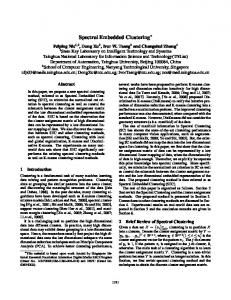
Figure 1: Two rectangular clusters intersecting at right angle. Left: the original data. Center: a typical output of the standard spectral clustering method of Ng et al. (2002), which is generally unable to resolve intersections. Right: our method.

estimation of the local linear structure (tangent bundle) via local principal component analysis (PCA). The idea of using local PCA combined with spectral clustering has precedents in the literature. In particular, our method is inspired by the work of Goldberg, Zhu, Singh, Xu, and Nowak (2009), where the authors develop a spectral clustering method within a semi-supervised learning framework. Local PCA is also used in the multiscale, spectral-flavored algorithm of Kushnir, Galun, and Brandt (2006). This approach is in the zeitgeist. While writing this paper, we became aware of two very recent publications, by Wang, Jiang, Wu, and Zhou (2011) and by Gong, Zhao, and Medioni (2012), both proposing approaches very similar to ours. We comment on these spectral methods in more detail later on. The basic proposition of local PCA combined with spectral clustering has two main stages. The first one forms an affinity between a pair of data points that takes into account both their Euclidean distance and a measure of discrepancy between their tangent spaces. Each tangent space is estimated by PCA in a local neighborhood around each point. The second stage applies standard spectral clustering with this affinity. As a reality check, this relatively simple algorithm succeeds at separating the straight clusters in Figure 1. We tested our algorithm in more elaborate settings, some of them described in Section 4. Besides spectral-type approaches to multi-manifold clustering, other methods appear in the literature. The methods we know of either assume that the different surfaces do not intersect (Polito and Perona, 2001), or that the intersecting surfaces have different intrinsic dimension or density (Gionis et al., 2005; Haro et al., 2007). The few exceptions tend to propose very complex methods that promise to be challenging to analyze (Guo et al., 2007; Souvenir and Pless, 2005). Our contribution is the design and detailed study of a prototypical spectral clustering algorithm based on local PCA, tailored to settings where the underlying clusters come from sampling in the vicinity of smooth surfaces that may intersect. We endeavored to simplify the algorithm as much as possible without sacrificing performance. We provide theoretical results for simpler variants within a standard mathematical framework for multi-manifold clustering. To our knowledge, these are the first mathematically backed successes at the task of resolving intersections in the context of multi-manifold clustering, with the exception of (Arias-Castro et al., 2011), where the corresponding algorithm is shown to succeed at identifying intersecting curves. The salient features of that algorithm are illustrated via numerical experiments. The rest of the paper is organized as follows. In Section 2, we introduce our methods. In Sec2

tion 3, we analyze our methods in a standard mathematical framework for multi-manifold learning. In Section 4, we perform some numerical experiments illustrating several features of our algorithm. In Section 5, we discuss possible extensions.

2

The methodology

We introduce our algorithm and simpler variants that are later analyzed in a mathematical framework. We start with some review of the literature, zooming in on the most closely related publications.

2.1

Some precedents

Using local PCA within a spectral clustering algorithm was implemented in four other publications we know of (Goldberg et al., 2009; Gong et al., 2012; Kushnir et al., 2006; Wang et al., 2011). As a first stage in their semi-supervised learning method, Goldberg, Zhu, Singh, Xu, and Nowak (2009) design a spectral clustering algorithm. The method starts by subsampling the data points, obtaining ‘centers’ in the following way. Draw y 1 at random from the data and remove its `-nearest neighbors from the data. Then repeat with the remaining data, obtaining centers y 1 , y 2 , . . . . Let C i denote the sample covariance in the neighborhood of y i made of its `-nearest neighbors. An m-nearest-neighbor graph is then defined on the centers in terms of the Mahalanobis distances. Explicitly, the centers y i and y j are connected in the graph if y j is among the m nearest neighbors of y i in Mahalanobis distance −1/2 (1) kC i (y i − y j )k, or vice-versa. The parameters ` and m are both chosen of order log n. An existing edge between y i and y j is then weighted by exp(−Hij2 /η 2 ), where Hij denotes the Hellinger distance between the probability distributions N (0, C i ) and N (0, C j ). The spectral graph partitioning algorithm of Ng, Jordan, and Weiss (2002) — detailed in Algorithm 1 — is then applied to the resulting affinity matrix, with some form of constrained K-means. We note that Goldberg et al. (2009) evaluate their method in the context of semi-supervised learning where the clustering routine is only required to return subclusters of actual clusters. In particular, the data points other than the centers are discarded. Note also that their evaluation is empirical. Algorithm 1

Spectral Graph Partitioning (Ng, Jordan, and Weiss, 2002)

Input: Affinity matrix W = (Wij ), size of the partition K Steps: p P 1: Compute Z = (Zij ) according to Zij = Wij / Di Dj , with Di = nj=1 Wij . 2: Extract the top K eigenvectors of Z. 3: Renormalize each row of the resulting n × K matrix. 4: Apply K-means to the row vectors. The algorithm proposed by Kushnir, Galun, and Brandt (2006) is multiscale and works by coarsening the neighborhood graph and computing sampling density and geometric information inferred along the way such as obtained via PCA in local neighborhoods. This bottom-up flow is then followed by a top-down pass, and the two are iterated a few times. The algorithm is too complex to be described in detail here, and probably too complex to be analyzed mathematically. 3

The clustering methods of Goldberg et al. (2009) and ours can be seen as simpler variants that only go bottom up and coarsen the graph only once. In the last stages of writing this paper, we learned of the works of Wang, Jiang, Wu, and Zhou (2011) and Gong, Zhao, and Medioni (2012), who propose algorithms very similar to our Algorithm 3 detailed below. Note that these publications do not provide any theoretical guarantees for their methods, which is one of our main contributions here.

2.2

Our algorithms

We now describe our method and propose several variants. Our setting is standard: we observe data points x1 , . . . , xn ∈ RD that we assume were sampled in the vicinity of K smooth surfaces embedded in RD . The setting is formalized later in Section 3.1. 2.2.1

Connected component extraction: comparing local covariances

We start with our simplest variant, which is also the most natural. The method depends on a neighborhood radius r > 0, a spatial scale parameter ε > 0 and a covariance (relative) scale η > 0. For a vector x, kxk denotes its Euclidean norm, and for a (square) matrix A, kAk denotes its spectral norm. For n ∈ N, we denote by [n] the set {1, . . . , n}. Given a data set x1 , . . . , xn , for any point x ∈ RD and r > 0, define the neighborhood Nr (x) = {xj : kx − xj k ≤ r}. Algorithm 2

(2)

Connected Component Extraction: Comparing Covariances

Input: Data points x1 , . . . , xn ; neighborhood radius r > 0; spatial scale ε > 0, covariance scale η > 0. Steps: 1: For each i ∈ [n], compute the sample covariance matrix C i of Nr (xi ). 2: Compute the following affinities between data points: Wij = 1I{kxi −xj k≤ε} · 1I{kC i −C j k≤ηr2 } .

(3)

3: Remove xi when there is xj such that kxj − xi k ≤ r and kC j − C i k > ηr2 . 4: Extract the connected components of the resulting graph. 5: Points removed in Step 3 are grouped with the closest point that survived Step 3. In summary, the algorithm first creates an unweighted graph: the nodes of this graph are the data points and edges are formed between two nodes if both the distance between these nodes and the distance between the local covariance structures at these nodes are sufficiently small. After removing the points near the intersection at Step 3, the algorithm then extracts the connected components of the graph. In principle, the neighborhood size r is chosen just large enough that performing PCA in each neighborhood yields a reliable estimate of the local covariance structure. For this, the number of points inside the neighborhood needs to be large enough, which depends on the sample size n, the sampling density, intrinsic dimension of the surfaces and their surface area (Hausdorff measure), how far the points are from the surfaces (i.e., noise level), and the regularity of the surfaces. The spatial scale parameter ε depends on the sampling density and r. It needs to be large enough that a 4

point has plenty of points within distance ε, including some across an intersection, so each cluster is strongly connected. At the same time, ε needs to be small enough that a local linear approximation to the surfaces is a relevant feature of proximity. Its choice is rather similar to the choice of the scale parameter in standard spectral clustering (Ng et al., 2002; Zelnik-Manor and Perona, 2004). The orientation scale η needs to be large enough that centers from the same cluster and within distance ε of each other have local covariance matrices within distance ηr2 , but small enough that points from different clusters near their intersection have local covariance matrices separated by a distance substantially larger than ηr2 . This depends on the curvature of the surfaces and the incidence angle at the intersection of two (or more) surfaces. Note that a typical covariance matrix over a ball of radius r has norm of order r2 , which justifies using our choice of parametrization. In the mathematical framework we introduce later on, these parameters can be chosen automatically as done in (Arias-Castro et al., 2011), at least when the points are sampled exactly on the surfaces. We will not elaborate on that since in practice this does not inform our choice of parameters. The rationale behind Step 3 is as follows. As we just discussed, the parameters need to be tuned so that points from the same cluster and within distance ε have local covariance matrices within distance ηr2 . Hence, xi and xj in Step 3 are necessarily from different clusters. Since they are near each other, in our model this will imply that they are close to an intersection. Therefore, roughly speaking, Step 3 removes points near an intersection. Although this method works in simple situations like that of two intersecting segments (Figure 1), it is not meant to be practical. Indeed, extracting connected components is known to be sensitive to spurious points and therefore unstable. Furthermore, we found that comparing local covariance matrices as in affinity (3) tends to be less stable than comparing local projections as in affinity (4), which brings us to our next variant.

2.2.2

Connected component extraction: comparing local projections

We present another variant also based on extracting the connected components of a neighborhood graph that compares orthogonal projections onto the largest principal directions. Algorithm 3

Connected Component Extraction: Comparing Projections

Input: Data points x1 , . . . , xn ; neighborhood radius r > 0, spatial scale ε > 0, projection scale η > 0. Steps: 1: For each i ∈ [n], compute the sample covariance matrix C i of Nr (xi ). √ 2: Compute the projection Qi onto the eigenvectors of C i with eigenvalue exceeding η kC i k. 3: Compute the following affinities between data points: Wij = 1I{kxi −xj k≤ε} · 1I{kQi −Qj k≤η} .

(4)

4: Extract the connected components of the resulting graph.

We note that the local intrinsic dimension is determined by thresholding the eigenvalues of the local covariance matrix, keeping the directions with eigenvalues within some range of the largest eigenvalue. The same strategy is used by Kushnir et al. (2006), but with a different threshold. The method is a hard version of what we implemented, which we describe next. 5

2.2.3

Covariances or projections?

In our numerical experiments, we tried working both directly with covariance matrices as in (3) and with projections as in (4). Note that in our experiments we used spectral graph partitioning with soft versions of these affinities, as described in Section 2.2.4. We found working with projections to be more reliable. The problem comes, in part, from boundaries. When a surface has a boundary, local covariances over neighborhoods that overlap with the boundary are quite different from local covariances over nearby neighborhoods that do not touch the boundary. Consider the example of two segments, S1 and S2 , intersecting at an angle of θ ∈ (0, π/2) at their middle point, specifically S1 = [−1, 1] × {0},

S2 = {(x, x tan θ) : x ∈ [− cos θ, cos θ]}.

Assume there is no noise and that the sampling is uniform. Assume r ∈ (0, 12 sin θ) so that the disc centered at x1 := (1/2, 0) does not intersect S2 , and the disc centered at x2 := ( 12 cos θ, 21 tan θ) does not intersect S1 . Let x0 = (1, 0). For x ∈ S1 ∪ S2 , let C x denote the local covariance at x over a ball of radius r. Simple calculations yield: C (1,0)

r2 = 12

1 0 , 0 0

C x1

r2 = 3

1 0 , 0 0

C x2

r2 = 3

and therefore kC x0

r2 − C x1 k = , 4

cos2 θ sin(θ) cos(θ) , sin(θ) cos(θ) sin2 θ

√ kC x1 − C x2 k =

2r2 sin θ. 3

3 When sin θ ≤ 4√ (roughly, θ ≤ 32o ), the difference in Frobenius norm between the local covariances 2 at x0 , x1 ∈ S1 is larger than that at x1 ∈ S1 and x2 ∈ S2 . As for projections, however,

Qx0 = Qx1 =

1 0 , 0 0

Qx2 =

cos2 θ sin(θ) cos(θ) , sin(θ) cos(θ) sin2 θ

so that kQx0 − Qx1 k = 0,

kQx1 − Qx2 k =

√

2 sin θ.

While in theory the boundary points account for a small portion of the sample, in practice this is not the case and we find that spectral graph partitioning is challenged by having points near the boundary that are far (in affinity) from nearby points from the same cluster. This may explain why the (soft version of) affinity (4) yields better results than the (soft version of) affinity (3) in our experiments. 2.2.4

Spectral Clustering Based on Local PCA

The following variant is more robust in practice and is the algorithm we actually implemented. The method assumes that the surfaces are of same dimension d and that they are K surfaces, with both parameters K and d known. We note that y 1 , . . . , y n0 forms an r-packing of the data. The underlying rationale for this coarsening is justified in (Goldberg et al., 2009) by the fact that the covariance matrices, and also the top principal directions, change smoothly with the location of the neighborhood, so that without subsampling these characteristics would not help detect the abrupt event of an intersection. The affinity (5) is of course a soft version of (4). 6

Algorithm 4

Spectral Clustering Based on Local PCA

Input: Data points x1 , . . . , xn ; neighborhood radius r > 0; spatial scale ε > 0, projection scale η > 0; intrinsic dimension d; number of clusters K. Steps: 0: Pick one point y 1 at random from the data. Pick another point y 2 among the data points not included in Nr (y 1 ), and repeat the process, selecting centers y 1 , . . . , y n0 . 1: For each i = 1, . . . , n0 , compute the sample covariance matrix C i of Nr (y i ). Let Qi denote the orthogonal projection onto the space spanned by the top d eigenvectors of C i . 2: Compute the following affinities between center pairs: ! ! ky i − y j k2 kQi − Qj k2 Wij = exp − · exp − . (5) ε2 η2 3: Apply spectral graph partitioning (Algorithm 1) to W . 4: The data points are clustered according to the closest center in Euclidean distance.

2.2.5

Comparison with closely related methods

We highlight some differences with the other proposals in the literature. We first compare our approach to that of Goldberg et al. (2009), which was our main inspiration. • Neighborhoods. Comparing with Goldberg et al. (2009), we define neighborhoods over rballs instead of `-nearest neighbors, and connect points over ε-balls instead of m-nearest neighbors. This choice is for convenience, as these ways are in fact essentially equivalent when the sampling density is fairly uniform. This is elaborated at length in (Arias-Castro, 2011; Brito et al., 1997; Maier et al., 2009). • Mahalanobis distances. Goldberg et al. (2009) use Mahalanobis distances (1) between centers. In our version, we could for example replace the Euclidean distance kxi − xj k in the affinity (3) with the average Mahalanobis distance −1/2

kC i

−1/2

(xi − xj )k + kC j

(xj − xi )k.

(6)

We actually tried this and found that the algorithm was less stable, particularly under low noise. Introducing a regularization in this distance — which requires the introduction of another parameter — solves this problem partially. That said, using Mahalanobis distances makes the procedure less sensitive to the choice of ε, in that neighborhoods may include points from different clusters. Think of two parallel line segments separated by a distance of δ, and assume there is no noise, so the points are sampled exactly from these segments. Assuming an infinite sample size, the local covariance is the same everywhere so that points within distance ε are connected by the affinity (3). Hence, Algorithm 2 requires that ε < δ. In terms of Mahalanobis distances, points on different segments are infinitely separated, so a version based on these distances would work with any ε > 0. In the case of curved surfaces and/or noise, the situation is similar, though not as evident. Even then, the gain in performance guarantees is not obvious, since we only require that ε be slightly larger in order of magnitude that r. 7

• Hellinger distances. As we mentioned earlier, Goldberg et al. (2009) use Hellinger distances of the probability distributions N (0, C i ) and N (0, C j ) to compare covariance matrices, specifically !1/2 1/4 D/2 det(C i C j ) 1−2 , (7) det(C i + C j )1/2 if C i and C j are full-rank. While using these distances or the Frobenius distances makes little difference in practice, we find it easier to work with the latter when it comes to proving theoretical guarantees. Moreover, it seems more natural to assume a uniform sampling distribution in each neighborhood rather than a normal distribution, so that using the more sophisticated similarity (7) does not seem justified. • K-means. We use K-means++ for a good initialization. However, we found that the more sophisticated size-constrained K-means (Bradley et al., 2000) used in (Goldberg et al., 2009) did not improve the clustering results. As we mentioned above, our work was developed in parallel to that of Wang et al. (2011) and Gong et al. (2012). We highlight some differences. They do not subsample, but estimate the local tangent space at each data point xi . Wang et al. (2011) fit a mixture of d-dimensional affine subspaces to the data using MPPCA (Tipping and Bishop, 1999), which is then used to estimate the tangent subspaces at each data point. Gong et al. (2012) develop some sort of robust local PCA. While Wang et al. (2011) assume all surfaces are of same dimension known to the user, Gong et al. (2012) estimate that locally by looking at the largest gap in the spectrum of estimated local covariance matrix. This is similar in spirit to what is done in Step 2 of Algorithm 3, but we did not include this step in Algorithm 4 because we did not find it reliable in practice. We also tried estimating the local dimensionality using the method of Little et al. (2009), but this failed in the most complex cases. Wang et al. (2011) use a nearest-neighbor graph and their affinity is defined as !α d Y Wij = ∆ij · cos θs (i, j) , (8) s=1

where ∆ij = 1 if xi is among the `-nearest neighbors of xj , or vice versa, while ∆ij = 0 otherwise; θ1 (i, j) ≥ · · · ≥ θd (i, j) are the principal (aka, canonical) angles (Stewart and Sun, 1990) between the estimated tangent subspaces at xi and xj . ` and α are parameters of the method. Gong et al. (2012) define an affinity that incorporates the self-tuning method of Zelnik-Manor and Perona (2004); in our notation, their affinity is ! asin2 kQi − Qj k kxi − xj k2 exp − · exp − 2 . (9) εi εj η kxi − xj k2 /(εi εj ) where εi is the distance from xi to its `-nearest neighbor. ` is a parameter. Although we do not analyze their respective ways of estimating the tangent subspaces, our analysis provides essential insights into their methods, and for that matter, any other method built on spectral clustering based on tangent subspace comparisons.

3

Mathematical Analysis

While the analysis of Algorithm 4 seems within reach, there are some complications due to the fact that points near the intersection may form a cluster of their own — we were not able to discard this 8

possibility. Instead, we study the simpler variants described in Algorithm 2 and Algorithm 3. Even then, the arguments are rather complex and interestingly involved. The theoretical guarantees that we thus obtain for these variants are stated in Theorem 1 and proved in Section 6. We comment on the analysis of Algorithm 4 right after that. We note that there are very few theoretical results on resolving intersecting clusters. In fact, we are only aware of (Chen and Lerman, 2009a) in the context of affine surfaces, (Soltanolkotabi and Cand`es, 2011) in the context of affine surfaces without noise and (Arias-Castro et al., 2011) in the context of curves. The generative model we assume is a natural mathematical framework for multi-manifold learning where points are sampled in the vicinity of smooth surfaces embedded in Euclidean space. For concreteness and ease of exposition, we focus on the situation where two surfaces (i.e., K = 2) of same dimension 1 ≤ d ≤ D intersect. This special situation already contains all the geometric intricacies of separating intersecting clusters. On the one hand, clusters of different intrinsic dimension may be separated with an accurate estimation of the local intrinsic dimension without further geometry involved (Haro et al., 2007). On the other hand, more complex intersections (3-way and higher) complicate the situation without offering truly new challenges. For simplicity of exposition, we assume that the surfaces are submanifolds without boundary, though it will be clear from the analysis (and the experiments) that the method can handle surfaces with (smooth) boundaries that may self-intersect. We discuss other possible extensions in Section 5. Within that framework, we show that Algorithm 2 and Algorithm 3 are able to identify the clusters accurately except for points near the intersection. Specifically, with high probability with respect to the sampling distribution, Algorithm 2 divides the data points into two groups such that, except for points within distance Cε of the intersection, all points from the first cluster are in one group and all points from the second cluster are in the other group. The constant C depends on the surfaces, including their curvatures, separation between them and intersection angle. The situation for Algorithm 3 is more complex, as it may return more than two clusters, but the main feature is that most of two clusters (again, away from the intersection) are in separate connected components.

3.1

Generative model

Each surface we consider is a connected, C 2 and compact submanifold without boundary and of dimension d embedded in RD . Any such surface has a positive reach, which is what we use to quantify smoothness. The notion of reach was introduced by Federer (1959). Intuitively, a surface has reach exceeding r if, and only if, one can roll a ball of radius r on the surface without obstruction (Walther, 1997). Formally, for x ∈ RD and S ⊂ RD , let dist(x, S) = inf kx − sk, s∈S

and B(S, r) = {x : dist(x, S) < r}, which is often called the r-tubular neighborhood (or r-neighborhood) of S. The reach of S is the supremum over r > 0 such that, for each x ∈ B(S, r), there is a unique point in S nearest x. It is well-known that, for C 2 submanifolds, the reach bounds the radius of curvature from below (Federer, 1959, Lem. 4.17). For submanifolds without boundaries, the reach coincides with the condition number introduced in (Niyogi et al., 2008). When two surfaces S1 and S2 intersect, meaning S1 ∩ S2 6= ∅, we define their incidence angle as θ(S1 , S2 ) := inf (θmin (TS1 (s), TS2 (s)) : s ∈ S1 ∩ S2 ) , 9

(10)

where TS (s) denote the tangent subspace of submanifold S at point s ∈ S, and θmin (T1 , T2 ) is the smallest nonzero principal (aka, canonical) angle between subspaces T1 and T2 (Stewart and Sun, 1990). The clusters are generated as follows. Each data point xi is drawn according to xi = si + z i ,

(11)

where si is drawn from the uniform distribution over S1 ∪ S2 and z i is an additive noise term satisfying kz i k ≤ τ — thus τ represents the noise or jitter level, and τ = 0 means that the points are sampled on the surfaces. We assume the points are sampled independently of each other. We let Ik = {i : si ∈ Sk }, (12) and the goal is to recover the groups I1 and I2 , up to some errors.

3.2

Performance guarantees

We state some performance guarantees for Algorithm 2 and Algorithm 3. Theorem 1. Consider two connected, compact, twice continuously differentiable submanifolds without boundary, of same dimension, intersecting at a strictly positive angle, with the intersection set having strictly positive reach. Assume the parameters are set so that τ ≤ rη/C,

r ≤ ε/C,

ε ≤ η/C,

η ≤ 1/C, and C > 0 is large enough. Then with probability at least 1 − Cn exp − nrd η 2 /C :

(13)

• Algorithm 2 returns exactly two groups such that two points from different clusters are not grouped together unless one of them is within distance Cr from the intersection. • Algorithm 3 returns at least two groups, and such that two points from different clusters are not grouped together unless one of them is within distance Cr from the intersection. We note that the constant C > 0 depends on what configuration the surfaces are in, in particular their reach and intersection angle, but also aspects that are harder to quantify, like their separation away from their intersection. We now comment on the challenge of proving a similar result for Algorithm 4. This algorithm relies on knowledge of the intrinsic dimension of the surfaces d and the number of clusters (here K = 2), but these may be estimated as in (Arias-Castro et al., 2011), at least in theory, so we assume these parameters are known. The subsampling done in Step 0 does not pose any problem whatsoever, since the centers are well-spread when the points themselves are. The difficulty resides in the application of the spectral graph partitioning, Algorithm 1. If we were to include the intersection-removal step (Step 3 of Algorithm 2) before applying spectral graph partitioning, then a simple adaptation of arguments in (Arias-Castro, 2011) would suffice. The real difficulty, and potential pitfall of the method in this framework (without the intersection-removal step), is that the points near the intersection may form their own cluster. For example, in the simplest case of two affine surfaces intersecting at a positive angle and no sampling noise, the projection matrix at a point near the intersection — meaning a point whose r-ball contains a substantial piece of both surfaces — would be the projection matrix onto S1 + S2 seen as a linear subspace. We were not able to discard this possibility, although we do not observe this happening in practice. A possible remedy is to constrain the K-means part to only return large-enough clusters. However, a proper analysis of this would require a substantial amount of additional work and we did not engage seriously in this pursuit. 10

4

Numerical Experiments

We tried our code§ on a few artificial examples. Very few algorithms were designed to work in the general situation we consider here and we did not compare our method with any other. As we argued earlier, the methods of Wang et al. (2011) and Gong et al. (2012) are quite similar to ours, and we encourage the reader to also look at the numerical experiments they performed. Our numerical experiments should be regarded as a proof of concept, only here to show that our method can be implemented and works on some toy examples. In all experiments, the number of clusters K and the dimension of the manifolds d are assumed known. We choose spatial scale ε and the projection scale η automatically as follows: we let ε = max min ky i − y j k, 1≤i≤n0 j6=i

(14)

and η=

median

(i,j):ky i −y j k 0, B(x, r) denotes the open ball of center x and radius r, i.e., B(x, r) = {y ∈ RD : ky − xk < r}. For a set S and a point x, define dist(x, S) = inf{kx − yk : y ∈ S}. For two points a, b in the same Euclidean space, b − a denotes the vector moving a to b. For a point a and a vector v in the same Euclidean space, a + v denotes the translate of a by v. We identify an affine subspace T with its corresponding linear subspace, for example, when saying that a vector belongs to T . For two subspaces T and T 0 , of possibly different dimensions, we denote by 0 ≤ θmax (T, T 0 ) ≤ π/2 the largest and by θmin (T, T 0 ) the smallest nonzero principal angle between T and T 0 (Stewart and Sun, 1990). When v is a vector and T is a subspace, ∠(v, T ) := θmax (Rv, T ) this is the usual definition of the angle between v and T . For a subset A ⊂ RD and positive integer d, vold (A) denotes the d-dimensional Hausdorff measure of A, and vol(A) is defined as voldim(A) (A), where dim(A) is the Hausdorff dimension of A. For a Borel set A, let λA denote the uniform distribution on A. For a set S ⊂ RD with reach at least 1/κ, and x with dist(x, S) < 1/κ, let PS (x) denote the metric projection of x onto S, that is, the point on S closest to x. Note that, if T is an affine subspace, then PT is the usual orthogonal projection onto T . Let Sd (κ) denote the class of connected, C 2 and compact d-dimensional submanifolds without boundary embedded in RD , with reach at least 1/κ. For a submanifold S ∈ RD , let TS (x) denote the tangent space of S at x ∈ S. We will often identify a linear map with its matrix in the canonical basis. For a symmetric (real) matrix M , let β1 (M ) ≥ β2 (M ) ≥ · · · denote its eigenvalues in decreasing order. We say that f : Ω ⊂ RD → RD is C-Lipschitz if kf (x) − f (y)k ≤ Ckx − yk, ∀x, y ∈ Ω. For two reals a and b, a ∨ b = max(a, b) and a ∧ b = min(a, b). Additional notation will be introduced as needed.

6.1

Preliminaries

This section gathers a number of general results from geometry and probability. We took time to package them into standalone lemmas that could be of potential independent interest, particularly to researchers working in machine learning and computational geometry. 6.1.1

Smooth surfaces and their tangent subspaces

The following result is on approximating a smooth surface near a point by the tangent subspace at that point. It is based on (Federer, 1959, Th. 4.18(2)). Lemma 1. For S ∈ Sd (κ), and any two points s, s0 ∈ S, dist(s0 , TS (s)) ≤

κ 0 ks − sk2 , 2

(16)

and when dist(s0 , TS (s)) ≤ 1/κ, dist(s0 , TS (s)) ≤ κkPTS (s) (s0 ) − sk2 .

(17)

Moreover, for t ∈ TS (s) such that ks − tk ≤ 7/(16κ), dist(t, S) ≤ κkt − sk2 . 16

(18)

Proof. Let T be short for TS (s). (Federer, 1959, Th. 4.18(2)) says that dist(s0 − s, T ) ≤

κ 0 ks − sk2 . 2

(19)

Immediately, we have dist(s0 − s, T ) = ks0 − PT (s0 )k = dist(s0 , T ), and (16) comes from that. Based on that and Pythagoras theorem, we have dist(s0 , T ) = kPT (s0 ) − s0 k ≤

κ 0 κ ks − sk2 = kPT (s0 ) − s0 k2 + kPT (s0 ) − sk2 , 2 2

so that dist(s0 , T ) 1 −

κ κ dist(s0 , T ) ≤ kPT (s0 ) − sk2 , 2 2

and (17) follows easily from that. For (18), let s0 = PT−1 (t), which is well-defined by Lemma 3 below and belongs to B(s, 1/(2κ)). We then apply (17) to get dist(t, S) ≤ kt − s0 k = dist(s0 , T ) ≤ κkt − sk2 .

We need a bound on the angle between tangent subspaces on a smooth surface as a function of the distance between the corresponding points of contact. This could be deduced directly from (Niyogi et al., 2008, Prop. 6.2, 6.3), but the resulting bound is much looser — and the underlying proof much more complicated — than the following, which is again based on (Federer, 1959, Th. 4.18(2)). Lemma 2. For S ∈ Sd (κ), and any s, s0 ∈ S, θmax (TS (s), TS (s0 )) ≤ 2 asin

κ 2

ks0 − sk ∧ 1 .

(20)

Proof. By (19) applied twice, we have dist(s0 − s, TS (s)) ∨ dist(s − s0 , TS (s0 )) ≤

κ 0 ks − sk2 . 2

Noting that dist(v, T ) = kvk sin ∠(v, T ),

(21)

for any vector v and any linear subspace T , we get sin ∠(s0 − s, TS (s)) ∨ sin ∠(s0 − s, TS (s0 )) ≤

κ 0 ks − sk. 2

Noting that the LHS never exceeds 1, and applying the arcsine function — which is increasing — on both sides, yields κ ∠(s0 − s, TS (s)) ∨ ∠(s0 − s, TS (s0 )) ≤ asin ks0 − sk ∧ 1 . 2 We then use the triangle inequality θmax (TS (s), TS (s0 )) ≤ ∠(s0 − s, TS (s)) + ∠(s0 − s, TS (s0 )), and conclude. 17

Below we state some properties of a projection onto a tangent subspace. A result similar to the first part was proved in (Arias-Castro et al., 2011, Lem. 2) based on results in (Niyogi et al., 2008), but the arguments are simpler here and the constants are sharper. 1 Lemma 3. Take S ∈ Sd (κ), s ∈ S and r ≤ 2κ , and let T be short for TS (s). PT is injective on 0 B(s, r) ∩ S and its image contains B(s, r ) ∩ T , where r0 := (1 − 12 (κr)2 )r. Moreover, PT−1 has 7 64 (κr)2 over B(s, r) ∩ T , for any r ≤ 16κ . Lipschitz constant bounded by 1 + 49

Proof. Take s0 , s00 ∈ S distinct such that PT (s0 ) = PT (s00 ). Equivalently, s00 − s0 is perpendicular to TS (s). Let T 0 be short for TS (s0 ). By (19) and (21), we have κ ks00 − s0 k ∧ 1 , ∠(s00 − s0 , T 0 ) ≤ asin 2 and by (20), θmax (T, T 0 ) ≤ 2 asin

κ 2

ks0 − sk ∧ 1 .

Now, by the triangle inequality, ∠(s00 − s0 , T 0 ) ≥ ∠(s00 − s0 , T ) − θmax (T, T 0 ) = so that

π − θmax (T, T 0 ), 2

κ

π κ ks00 − s0 k ∧ 1 ≥ − 2 asin ks0 − sk ∧ 1 . 2 2 2 0 When ks −sk ≤ 1/κ, the RHS is bounded from below by π/2−2 asin(1/2), which then implies that κ 00 0 00 0 2 ks − s k ≥ sin(π/2 − 2 asin(1/2)) = 1/2, that is, ks − s k ≥ 1/κ. This precludes the situation where s0 , s00 ∈ B(s, 1/(2κ)), so that PT is injective on B(s, r) when r ≤ 1/(2κ). The same arguments imply that PT is an open map on R := B(s, r) ∩ S. In particular, PT (R) contains an open ball in T centered at s and PT (∂R) = ∂PT (R), with ∂R = S ∩ ∂B(s, r) since ∂S = ∅. Now take any ray out of s within T , which is necessarily of the form s + Rv, where v is a unit vector in T . Let ta = s + av ∈ T for a ∈ [0, ∞). Let a∗ be the infimum over all a > 0 such that ta ∈ PT (R). Note that a∗ > 0 and ta∗ ∈ PT (∂R), so that there is s∗ ∈ ∂R such that PT (s∗ ) = ta∗ . Let s(a) = PT−1 (s + av), which is well-defined on [0, a∗ ] by definition of a∗ and the fact that PT is ˙ injective on R. We have that s(a) = Dta PT−1 v is the unique vector in Ta := TS (PT−1 (ta )) such that ˙ PT (s(a)) = v. Elementary geometry shows that asin

˙ ˙ ˙ ˙ kPT (s(a))k = ks(a)k cos ∠(s(a), T ) ≥ ks(a)k cos θmax (Ta , T ), with

h κ i 1 cos θmax (Ta , T ) ≥ cos 2 asin ks(a) − sk ≥ ζ := 1 − (κr)2 , 2 2 2 ˙ by (20), ks(a) − sk ≤ r and cos[2 asin(x)] = 1 − 2x when 0 ≤ x ≤ 1. Since kPT (s(a))k = kvk = 1, ˙ we have ks(a)k ≤ 1/ζ, and this holds for all a < a∗ . So we can extend s(a) to [0, a∗ ] into a Lipschitz function with constant 1/ζ. Together with the fact that s∗ ∈ ∂B(s, r), this implies that r = ks∗ − sk = ks(a∗ ) − s(0)k ≤

a∗ 1 ka∗ vk = . ζ ζ

Hence, a∗ ≥ ζr and therefore PT (R) contains B(s, ζr) ∩ T as stated. 7 For the last part, fix r < 16 κ, so there is a unique h < 1/(2κ) such that ζh = r, where ζ is 1 2 redefined as ζ := 1 − 2 (κh) . Take t0 ∈ B(s, r) ∩ T and let s0 = PT−1 (t0 ) and T 0 = TS (s0 ). We saw that PT−1 is Lipschitz with constant 1/ζ on any ray from s of length r, so that ks0 − sk ≤ 18

(1/ζ)kt0 − sk ≤ r/ζ = h. The differential of PT at s0 is PT itself, seen as a linear map between T 0 and T . Then for any vector u ∈ T 0 , we have kPT (u)k = kuk cos ∠(u, T ) ≥ kuk cos θmax (T 0 , T ), with

h κ i 1 cos θmax (T 0 , T ) ≥ cos 2 asin ks0 − sk ≥ 1 − (κh)2 = ζ, 2 2

as before. Hence, kDt0 PT−1 k ≤ 1/ζ, and we proved this for all t0 ∈ B(s, r) ∩ T . Since that set is convex, we can apply Taylor’s theorem and get that PT−1 is Lipschitz on that set with constant 1/ζ. We then have 64 1/ζ ≤ 1 + (κh)2 ≤ 1 + (κr)2 , 49 because κh ≤ 1/2 and r = ζh ≥ 7h/8. 6.1.2

Volumes and uniform distributions

Below is a result that quantifies how much the volume of a set changes when applying a Lipschitz map. This is well-known in measure theory and we only provide a proof for completeness. Lemma 4. Suppose Ω is a measurable subset of RD and f : Ω ⊂ RD → RD is C-Lipschitz. Then for any measurable set A ⊂ Ω and real d > 0, vold (f (A)) ≤ C d vold (A). Proof. By definition, vold (A) = lim Vdt (A), t→0

Vdt (A) :=

inf

X

(Ri )∈Rt (A)

diam(Ri )d ,

i∈N

S where Rt (A) is the class of countable sequences (Ri : i ∈ N) of subsets of RD such that A ⊂ i Ri and diam(Ri ) < t for all i. Since f is C-Lipschitz, diam(f (R)) ≤ C diam(R) for any R ⊂ Ω. Hence, for any (Ri ) ∈ Rt (A), (f (Ri )) ∈ RCt (f (A)). This implies that VdCt (f (A)) ≤

X

diam(f (Ri ))d ≤ C d

i∈N

X

diam(Ri )d .

i∈N

Taking the infimum over (Ri ) ∈ Rt (A), we get VdCt (f (A)) ≤ C d Vdt (A), and we conclude by taking the limit as t → 0, noticing that VdCt (f (A)) → vol(f (A)). We compare below two uniform distributions. For two Borel probability measures P and Q on RD , TV(P, Q) denotes their total variation distance, meaning, TV(P, Q) = sup{|P (A) − Q(A)| : A Borel set}. Remember that for a Borel set A, λA denotes the uniform distribution on A. Lemma 5. Suppose A and B are two Borel subsets of RD . Then TV(λA , λB ) ≤ 4

19

vol(A 4 B) . vol(A ∪ B)

Proof. If A and B are not of same dimension, say dim(A) > dim(B), then TV(λA , λB ) = 1 since λA (B) = 0 while λB (B) = 1. And we also have vol(A 4 B) = voldim(A) (A 4 B) = voldim(A) (A) = vol(A), and vol(A ∪ B) = voldim(A) (A ∪ B) = voldim(A) (A) = vol(A), in both cases because voldim(A) (B) = 0. So the result works in that case. Therefore assume that A and B are of same dimension. Assume WLOG that vol(A) ≥ vol(B). For any Borel set U , vol(A ∩ U ) vol(B ∩ U ) λA (U ) − λB (U ) = − , vol(A) vol(B) so that |λA (U ) − λB (U )| ≤ ≤ ≤

1 1 | vol(A ∩ U ) − vol(B ∩ U )| + vol(B ∩ U ) − vol(A) vol(A) vol(B) vol(A 4 B) vol(B ∩ U ) | vol(A) − vol(B)| + vol(A) vol(B) vol(A) 2 vol(A 4 B) , vol(A)

and we conclude with the fact that vol(A ∪ B) ≤ vol(A) + vol(B) ≤ 2 vol(A). We now look at the projection of the uniform distribution on a neighborhood of a surface onto a tangent subspace. For a Borel probability measure P and measurable function f : RD → RD , P f denotes the push-forward (Borel) measure defined by P f (A) = P (f −1 (A)). Lemma 6. Suppose A ⊂ RD is Borel and f : A → RD is invertible on f (A), and that both f and f −1 are C-Lipschitz. Then TV(λfA , λf (A) ) ≤ 8(C dim(A) − 1). Proof. First, note that A and f (A) are both of same dimension, and that C ≥ 1 necessarily. Let d be short for dim(A). Take U ⊂ f (A) Borel and let V = f −1 (U ). Then λfA (U ) =

vol(A ∩ V ) , vol(A)

|λfA (U ) − λf (A) (U )| ≤

λf (A) (U ) =

vol(f (A) ∩ U ) , vol(f (A))

| vol(A ∩ V ) − vol(f (A) ∩ U )| | vol(A) − vol(f (A))| + . vol(A) vol(A)

f being invertible, we have f (A ∩ V ) = f (A) ∩ U and f −1 (f (A) ∩ U ) = A ∩ V . Therefore, applying Lemma 4, we get vol(f (A) ∩ U ) ≤ C d, C −d ≤ vol(A ∩ V ) so that | vol(A ∩ V ) − vol(f (A) ∩ U )| ≤ (C d − 1) vol(A ∩ V ) ≤ (C d − 1) vol(A). Similarly, | vol(A) − vol(f (A))| ≤ (C d − 1) vol(A). We then conclude with Lemma 5. 20

Now comes a technical result on the intersection of a smooth surface and a ball. Lemma 7. There is a constant C7 ≥ 3 depending only on d such that the following is true. Take S ∈ Sd (κ), r < C17 κ and x ∈ RD such that dist(x, S) < r. Let s = PS (x) and T = TS (s). Then vol PT (S ∩ B(x, r)) 4 (T ∩ B(x, r)) ≤ C7 (kx − sk + r2 ) vol(T ∩ B(x, r)). Proof. Let Ar = B(s, r), Br = B(x, r) and g = PT for short. Note that T ∩ Br = T ∩ Ar0 where r0 := (r2 − δ 2 )1/2 and δ := kx − sk. Take s1 ∈ S ∩ Br such that g(s1 ) is farthest from s, so that g(S ∩ Br ) ⊂ Ar1 where r1 := ks − g(s1 )k — note that r1 ≤ r. Let `1 = ks1 − g(s1 )k and y 1 be the orthogonal projection of s1 onto the line (x, s). By Pythagoras theorem, we have kx − s1 k2 = kx − y 1 k2 + ky 1 − s1 k2 . We have kx − s1 k ≤ r and ky 1 − s1 k = ks − g(s1 )k = r1 . And because `1 ≤ κr12 < r by (17), either y 1 is between x and s, in which case kx − y 1 k = δ − `1 , or s is between x and y 1 , in which case kx − y 1 k = δ + `1 . In any case, r2 ≥ r12 + (δ − `1 )2 , which together with `1 ≤ κr12 implies r12 ≤ r2 −δ 2 +2δ`1 ≤ r02 +2κr12 δ, leading to r1 ≤ (1−2κδ)−1/2 r0 ≤ (1+4κδ)r0 after noticing that δ ≤ r < 1/(3κ). From g(S ∩ Br ) ⊂ T ∩ Ar1 , we get vol g(S ∩ Br ) \ (T ∩ Br ) ≤ vol(T ∩ Ar1 ) − vol(T ∩ Ar0 ) = ((r1 /r0 )d − 1) vol(T ∩ Ar0 ). We follow similar arguments to get a sort of reverse relationship. Take s2 ∈ S ∩ Br such that g(S ∩ Br ) ⊃ T ∩ Ar2 , where r2 := ks − g(s2 )k is largest. Assuming r is small enough, by Lemma 3, g −1 is well-defined on T ∩ Ar , so that necessarily s2 ∈ ∂Br . Let `2 = ks2 − g(s2 )k and y 2 be the orthogonal projection of s2 onto the line (x, s). By Pythagoras theorem, we have kx − s2 k2 = kx − y 2 k2 + ky 2 − s2 k2 . We have kx − s2 k = r and ky 2 − s2 k = ks − g(s2 )k = r2 . And by the triangle inequality, kx − y 2 k ≤ kx − sk + ky 2 − sk = δ + `2 . Hence, r2 ≤ r22 + (δ + `2 )2 , which together with `2 ≤ κr22 by (17), implies r22 ≥ r2 − δ 2 − 2δ`2 − `22 ≥ r02 − (2δ + κr2 )κr22 , leading to r2 ≥ (1 + 2κδ + κ2 r2 )−1/2 r0 ≥ (1 − 2κδ − κ2 r2 )r0 . From g(S ∩ Br ) ⊃ T ∩ Ar2 , we get vol (T ∩ Br ) \ g(S ∩ Br ) ≤ vol(T ∩ Ar0 ) − vol(T ∩ Ar2 ) = (1 − (r2 /r0 )d ) vol(T ∩ Ar0 ). All together, we have vol g(S ∩ Br ) 4 (T ∩ Br )

≤ ≤

(r1 /r0 )d − (r2 /r0 )d

vol(T ∩ Ar0 ) (1 + 4κδ)d − (1 − 2κδ − κ2 r2 )d vol((T ∩ Br )),

with (1 + 4κr)d − (1 − 4κr)d ≤ C(δ + r2 ) when δ ≤ r ≤ 1/(3κ), for a constant C depending only on d and κ. The result follows from this. We bound below the d-volume of a the intersection of a ball with a smooth surface. Though it could be obtained as a special case of Lemma 7, we provide a direct proof because this result is at the cornerstone of many results in the literature on sampling points uniformly on a smooth surface. Lemma 8. Suppose S ∈ Sd (κ). Then for any s ∈ S and r < 1 − 2dκr ≤

1 (d∨3)κ ,

we have

vol(S ∩ B(s, r)) ≤ 1 + 2dκr, vol(T ∩ B(s, r))

where T := TS (s) is the tangent subspace of S at s. 21

Proof. Let T = TS (s), Br = B(s, r) and g = PT for short. By Lemma 3, g is bi-Lipschitz with constants (1 + κr)−1 and 1 on S ∩ Br , so by Lemma 4 we have (1 + κr)−d ≤

vol(g(S ∩ Br )) ≤ 1. vol(S ∩ Br )

That g −1 is Lipschitz with constant 1 + κr on g(S ∩ Br ) also implies that g(S ∩ Br ) contains T ∩ Br0 where r0 := r/(1 + κr). From this, and the fact that g(S ∩ Br ) ⊂ T ∩ Br , we get 1≤

vol(T ∩ Br ) vol(T ∩ Br ) rd ≤ = d = (1 + κr)d . vol(g(S ∩ Br )) vol(T ∩ Br0 ) r0

(22)

We therefore have vol(S ∩ Br ) ≥ vol(g(S ∩ Br )) ≥ (1 + κr)−d vol(T ∩ Br ), and vol(S ∩ Br ) ≤ (1 + κr)d vol(g(S ∩ Br )) ≤ (1 + κr)d vol(T ∩ Br ). And we conclude with the inequality (1 + x)d ≤ 1 + 2dx valid for any x ∈ [0, 1/d] and any d ≥ 1. We now look at the density of a sample from the uniform on a smooth, compact surface. Lemma 9. There is a constant C9 > 0 such that the following is true. If S ∈ Sd (κ) and we sample n points s1 , . . . , sn independently and uniformly at random from S, and if 0 < r < 1/(C9 κ), then with probability at least 1 − C9 r−d exp(−nrd /C9 ), any ball of radius r with center on S has between nrd /C9 and C9 nrd sample points. Proof. For a set R, let N (R) denote the number of sample points in R. For any R measurable, N (R) ∼ Bin(n, pR ), where pR := vol(R ∩ S)/ vol(S). Let x1 , . . . , xm be an (r/2)-packing of S, and let Bi = B(xj , r/4) ∩ S. For any s ∈ S, there is j such that ks − xj k ≤ r/2, which implies Bi ⊂ B(s, r) by the triangle inequality. Hence, mins∈S N (B(s, r)) ≥ mini N (Bi ). By the fact that Bi ∩ Bj = ∅ for i 6= j, vol(S) ≥

m X

vol(Bi ) ≥ m min vol(Bi ), i

i=1

and assuming that r is small enough that we may apply Lemma 8, we have min vol(Bi ) ≥ i

ωd (r/4)d , 2

where ωd is the volume of the d-dimensional unit ball. This leads to m ≤ Cr−d and p := mini pBi ≥ rd /C, where C > 0 depends only on S. Now, applying Bernstein’s inequality to the binomial distribution, we get P (N (Bi ) ≤ np/2) ≤ P (N (Bi ) ≤ npBi /2) ≤ e−(3/32)npBi ≤ e−(3/32)np . We follow this with the union bound, to get 3 d d P min N (B(s, r)) ≤ nr /(2C) ≤ me−(3/32)np ≤ Cr−d e− 32C nr . s∈S

From this the lower bound follows. The proof of the upper bound is similar. 22

(23)

Next, we bound the volume of the symmetric difference between two balls. Lemma 10. Take x, y ∈ Rd and 0 < δ ≤ 1. Then vol(B(x, δ) 4 B(y, 1)) ≤ 1 − (1 − kx − yk)d+ ∧ δ d . 2 vol(B(0, 1)) Proof. It suffices to prove the result when kx − yk < 1. In that case, with γ := (1 − kx − yk) ∧ δ, we have B(x, γ) ⊂ B(x, δ) ∩ B(y, 1), so that vol(B(x, δ) 4 B(y, 1)) = vol(B(x, δ)) + vol(B(y, 1)) − 2 vol(B(x, δ) ∩ B(y, 1)) ≤ 2 vol(B(y, 1)) − 2 vol(B(x, γ)) = 2 vol(B(y, 1))(1 − γ d ).

6.1.3

Covariances

The result below describes explicitly the covariance matrix of the uniform distribution over the unit ball of a subspace. Lemma 11. Let T be a subspace of dimension d. Then the covariance matrix of the uniform 1 distribution on T ∩ B(0, 1) (seen as a linear map) is equal to cPT , where c := d+2 . Proof. Assume WLOG that T = Rd × {0}. Let X be distributed according to the uniform distribution on T ∩ B(0, 1) and let R = kXk. Note that P (R ≤ r) =

vol(T ∩ B(0, r)) = rd , vol(T ∩ B(0, 1))

∀r ∈ [0, 1].

By symmetry, E(Xi Xj ) = 0 if i 6= j, while E(X12 )

1 1 1 = E(X12 + · · · + Xd2 ) = E(R2 ) = d d d

This is exactly the representation of

1 d+2 PT

Z

1

r2 · drd−1 dr =

0

1 . d+2

in the canonical basis of RD .

We now show that a bound on the total variation distance between two compactly supported distributions implies a bound on the difference between their covariance matrices. For a measure P on RD and an integrable function f , let P (f ) denote the integral of f with respect to P , that is, Z P (f ) = f (x)P (dx), and let E(P ) = P (x) and Cov(P ) = P (xx> ) − P (x)P (x)> denote the mean and covariance matrix of P , respectively. Lemma 12. Suppose λ and ν are two Borel probability measures on Rd supported on B(0, 1). Then √ k E(λ) − E(ν)k ≤ d TV(λ, ν), k Cov(λ) − Cov(ν)k ≤ 3d TV(λ, ν). 23

Proof. Let fk (t) = tk when t = (t1 , . . . , td ), and note that |fk (t)| ≤ 1 for all k and all t ∈ B(0, 1). By the fact that TV(λ, ν) = sup{λ(f ) − ν(f ) : f : Rd → R measurable with |f | ≤ 1}, we have |λ(fk ) − ν(fk )| ≤ TV(λ, ν),

∀k = 1, . . . , d.

Therefore, d X k E(λ) − E(ν)k = (λ(fk ) − ν(fk ))2 ≤ d TV(λ, ν)2 , 2

k=1

which proves the first part. Similarly, let fk` (t) = tk t` . Since |fk` (t)| ≤ 1 for all k, ` and all t ∈ B(0, 1), we have |λ(fk` ) − ν(fk` )| ≤ TV(λ, ν),

∀k, ` = 1, . . . , d.

Since for any probability measure µ on Rd , Cov(µ) = µ(fk` ) − µ(fk )µ(f` ) : k, ` = 1, . . . , d , we have k Cov(λ) − Cov(ν)k ≤ d max |λ(fk` ) − ν(fk` )| + |λ(fk )λ(f` ) − ν(fk )ν(f` )| k,`

≤ d max |λ(fk` ) − ν(fk` )| + |λ(fk )||λ(f` ) − ν(f` )| + |ν(f` )||λ(fk ) − ν(fk )| k,`

≤ 3d TV(λ, ν), using the fact that |λ(fk )| ≤ 1 and |ν(fk )| ≤ 1 for all k. Next we compare the covariance matrix of the uniform distribution on a small piece of smooth surface with that of the uniform distribution on the projection of that piece onto a nearby tangent subspace. Lemma 13. There is a constant C13 > 0 depending only on d such that the following is true. Take 1 D such that dist(x, S) ≤ r. Let s = P (x) and T = T (s). If ζ S ∈ Sd (κ), r < C13 S S κ and x ∈ R and ξ are the means, and M and N are the covariance matrices of the uniform distributions on S ∩ B(x, r) and T ∩ B(x, r) respectively, then kζ − ξk ≤ C13 κr2 ,

kM − N k ≤ C13 κr3 .

Proof. We focus on proving the bound on the covariances, and leave the bound on the means — whose proof is both similar and simpler — as an exercise to the reader. Let T = TS (s), Br = B(x, r) and g = PT for short. Let A = S ∩ Br and A0 = T ∩ Br . Let X ∼ λA and define Y = g(X) with distribution denoted λgA . We have Cov(X) − Cov(Y ) =

1 Cov(X − Y, X + Y ) + Cov(X + Y, X − Y ) , 2

where Cov(U, V ) = E((U − µU )(V − µV )T ) is the cross-covariance of random vectors U and V with respective means µU and µV . Note that by Jensen’s inequality, the fact kuv T k = kukkvk for any pair of vectors u, v, and then the Cauchy-Schwarz inequality k Cov(U, V )k ≤ E(kU − µU k · kV − µV k) ≤ E(kU − µU k2 )1/2 · E(kV − µV k2 )1/2 . 24

Hence, letting µX = E X and µY = E Y , we have k Cov(λA ) − Cov(λgA )k ≤ k Cov(X − Y, X + Y )k 1/2 1/2 ≤ E kX − Y − µX + µY k2 E kX + Y − µX − µY k2 1/2 1/2 1/2 ≤ E kX − Y k2 E kX − sk2 + E kY − sk2 (24) κ 2 r r + r) = κr3 , ≤ 2 where the third inequality is due to the triangle inequality and fact that the mean minimizes the mean-squared error, and the third to the fact that X, Y ∈ Br and (16). Assume r < 1/((C7 ∨ d)κ). Let λg(A) denote the uniform distribution on g(A). λgA and λg(A) are both supported on Br , so that applying Lemma 12 with proper scaling, we get k Cov(λgA ) − Cov(λg(A) )k ≤ 3dr2 TV(λgA , λg(A) ). We know that g is 1-Lipschitz, and by Lemma 3 — which is applicable since C7 ≥ 3 — g −1 is well-defined and is (1 + κr)-Lipschitz on Br . Hence, by Lemma 6 and the fact that dim(A) = d, we have TV(λgA , λg(A) ) ≤ 8((1 + κr)d − 1) ≤ 16dκr, using the inequality (1 + x)d ≤ 1 + 2dx, valid for any x ∈ [0, 1/d] and any d ≥ 1. Noting that λA0 is also supported on Br , applying Lemma 12 with proper scaling, we get k Cov(λg(A) ) − Cov(λA0 )k ≤ 3dr2 TV(λg(A) , λA0 ), with TV(λg(A) , λA0 ) ≤ 4

vol(A 4 A0 ) ≤ Cκr, vol(A0 )

by Lemma 5 and Lemma 7, where C depends only on d, κ. By the triangle inequality, kM − N k = k Cov(λA ) − Cov(λA0 )k ≤ k Cov(λA ) − Cov(λgA )k + k Cov(λgA ) − Cov(λg(A) )k + k Cov(λg(A) ) − Cov(λA0 )k ≤ κr3 + 48d2 κr3 + Cr3 . From this, we conclude. Next is a lemma on the estimation of a covariance matrix. The result is a simple consequence of the matrix Hoeffding inequality of Tropp (2012). Note that simply bounding the operator norm by the Frobenius norm, and then applying the classical Hoeffding inequality (Hoeffding, 1963) would yield a bound sufficient for our purposes, but this is a good opportunity to use a more recent and sophisticated result. Lemma 14. Let C m denote the empirical covariance matrix based on an i.i.d. sample of size m from a distribution on the unit ball of Rd with covariance Σ. Then t m mt min , . P (kC m − Σk > t) ≤ 4d exp − 16 32 d 25

Proof. Without loss of generality, we assume that the distribution has zero mean and is now supported on B(0, 2). Let x1 , . . . , xm denote the sample, with xi = (xi,1 , . . . , xi,d ). We have C m = C ?m − where

m

C ?m

1 X := xi xTi , m i=1

1 ¯x ¯T , x m m

1 X ¯ := x xi . m i=1

Note that

1 k¯ xk2 . m Applying the union bound and then Hoeffding’s inequality to each coordinate — which is in [−2, 2] — we get d X √ mt2 . P(k¯ xk > t) ≤ P(|¯ xj | > t/ d) ≤ 2d exp − 8d kC m − Σk ≤ kC ?m − Σk +

j=1

1 T m (xi xi

Noting that − Σ), i = 1, . . . , m, are independent, zero-mean, self-adjoint matrices with spectral norm bounded by 4/m, we may apply the matrix Hoeffding inequality (Tropp, 2012, Th. 1.3), we get t2 ? P (kC m − Σk > t) ≤ 2d exp − 2 , σ 2 := m(4/m)2 = 16/m. 8σ Applying the union bound and using the previous inequalities, we arrive at p P (kC m − Σk > t) ≤ P (kC ?m − Σk > t/2) + P k¯ xk > mt/2 mt2 m2 t ≤ 2d exp − + 2d exp − 512 16d mt t m ≤ 4d exp − min , . 16 32 d

6.1.4

Projections

We relate below the difference of two orthogonal projections with the largest principal angle between the corresponding subspaces. Lemma 15. For two affine non-null subspaces T, T 0 , ( sin θmax (T, T 0 ), if dim(T ) = dim(T 0 ), kPT − PT 0 k = 1, otherwise. Proof. For two affine subspaces T, T 0 ⊂ RD of same dimension, let π2 ≥ θ1 ≥ · · · ≥ θD ≥ 0, denote the principal angles between them. By (Stewart and Sun, 1990, Th. I.5.5), the singular values of PT − PT 0 are {sin θj : j = 1, . . . , q}, so that kPT − PT 0 k = maxj sin θj = sin θ1 = sin θmax (T, T 0 ). Suppose now that T and T 0 are of different dimension, say dim(T ) > dim(T 0 ). We have kPT −PT 0 k ≤ kPT k ∨ kPT 0 k = 1, since PT and PT 0 are orthogonal projections and therefore positive semidefinite with operator norm equal to 1. Let L = PT (T 0 ). Since dim(L) ≤ dim(T 0 ) < dim(T ), there is u ∈ T ∩ L⊥ with u 6= 0. Then v > u = PT (v)> u = 0 for all v ∈ T 0 , implying that PT 0 (u) = 0 and consequently (PT − PT 0 )u = u, so that kPT − PT 0 k ≥ 1. 26

The lemma below is a perturbation result for eigenspaces and widely known as the sin Θ Theorem of Davis and Kahan (1970). See also (Luxburg, 2007, Th. 7) or (Stewart and Sun, 1990, Th. V.3.6). Lemma 16 (Davis and Kahan). Let M be positive semi-definite with eigenvalues β1 ≥ β2 ≥ · · · . Suppose that ∆d := βd − βd+1 > 0. Then for any other positive semi-definite matrix N , √ 2kN − M k (d) (d) kPN − PM k ≤ , ∆d (d)

(d)

where PM and PM denote the orthogonal projections onto the top d eigenvectors of M and N , respectively. 6.1.5

Intersections

We start with an elementary result on points near the intersection of two affine subspaces. Lemma 17. Take any two linear subspaces T1 , T2 ⊂ RD . For any point t1 ∈ T1 \ T2 , we have dist(t1 , T2 ) ≥ dist(t1 , T1 ∩ T2 ) sin θmin (T1 , T2 ). Proof. We may reduce the problem to the case where T1 ∩ T2 = {0}. Indeed, let T˜1 = T1 ∩ T2⊥ , T˜2 = T1⊥ ∩ T2 and ˜t1 = t1 − PT1 ∩T2 (t1 ). Then kt1 − PT2 (t1 )k = k˜t1 − PT˜2 (˜t1 )k,

kt1 − PT1 ∩T2 (t1 )k = k˜t1 k,

sin θmin (T1 , T2 ) = sin θmin (T˜1 , T˜2 ).

So assume that T1 ∩ T2 = {0}. By (Afriat, 1957, Th. 10.1), the angle formed by t1 and PT2 (t1 ) is at least as large as the smallest principal angle between T1 and T2 , which is θmin (T1 , T2 ) since T1 ∩ T2 = {0}. From this the result follows immediately. The following result says that a point cannot be close to two compact and smooth surfaces intersecting at a positive angle without being close to their intersection. Note that the constant there cannot be solely characterized by κ, as it also depends on the separation between the surfaces away from their intersection. Lemma 18. Suppose S1 , S2 ∈ Sd (κ) intersect at a strictly positive angle and that reach(S1 ∩ S2 ) ≥ 1/κ. Then there is a constant C18 such that dist(x, S1 ∩ S2 ) ≤ C18 max dist(x, S1 ), dist(x, S2 ) , ∀x ∈ RD . (25) Proof. Assume the result is not true, so there is a sequence (xn ) ⊂ RD such that dist(xn , S1 ∩S2 ) > n maxk dist(xn , Sk ). Because the surfaces are bounded, we may assume WLOG that the sequence is bounded. Then dist(xn , S1 ∩ S2 ) is bounded, which implies maxk dist(xn , Sk ) = O(1/n). This also forces dist(xn , S1 ∩ S2 ) → 0. Indeed, otherwise there is a constant C > 0 and a subsequence (xn0 ) such that dist(xn0 , S1 ∩ S2 ) ≥ C. Since (xn0 ) is bounded, there is a subsequence (xn00 ) that converges, and by the fact that maxk dist(xn00 , Sk ) = o(1), and by compactness of Sk , the limit is necessarily in S1 ∩ S2 , which is a contradiction. So we have dist(xn , S1 ∩ S2 ) = o(1), implying maxk dist(xn , Sk ) = o(1/n). Assume n is large enough that dist(xn , S1 ∩ S2 ) < 1/κ and let skn be the projection of xn onto Sk , and s‡n the projection of xn onto S1 ∩ S2 . Let Tk = TSk (s‡n ) and note that θmin (T1 , T2 ) ≥ θ, where θ > 0 is the minimum intersection angle between S1 and S2 defined in (10). Let tkn be the 27

projection of skn onto Tk . Assume WLOG that kt1n − s1n k ≥ kt2n − s2n k. Let tn denote the projection of t1n onto T1 ∩ T2 , and then let sn = PS1 ∩S2 (tn ). By assumption, we have n max kxn − skn k ≤ kxn − s‡n k = o(1). k

(26)

We start with the RHS: kxn − s‡n k =

min kxn − sk ≤ kxn − sn k,

s∈S1 ∩S2

(27)

and first show that kxn − sn k = o(1) too. We use the triangle inequality multiple times in what follows. We have kxn − sn k ≤ kxn − s1n k + ks1n − t1n k + kt1n − tn k + ktn − sn k.

(28)

From (26), kxn − s1n k = o(1) and kxn − s‡n k = o(1), and so that by (16), ks1n − t1n k ≤ κks1n − s‡n k2 ≤ 2κ(ks1n − xn k2 + kxn − s‡n k2 ) = o(1).

(29)

We also have kt1n − tn k = min kt1n − tk ≤ kt1n − s‡n k ≤ kt1n − s1n k + ks1n − xn k + kxn − s‡n k = o(1), t∈T1 ∩T2

(30)

where the first inequality comes from s‡n ∈ T1 ∩ T2 . Finally, ktn − sn k =

min ktn − sk ≤ ktn − s‡n k ≤ ktn − t1n k + kt1n − s‡n k = o(1),

s∈S1 ∩S2

where the first inequality comes from s‡n ∈ S1 ∩ S2 . We now proceed. The last upper bound is rather crude. Indeed, we use (18) for S = S1 ∩ S2 and s = s‡n , noting that TS1 ∩S2 (s‡n ) = T1 ∩ T2 and ktn − s‡n k = o(1), and get ktn − sn k ≤ κktn − s‡n k2 ≤ κ(ktn − sn k + ksn − xn k + kxn − s‡n k)2 . We have kxn − s‡n k = kxn − PS1 ∩S2 (xn )k ≤ kxn − sn k because sn ∈ T1 ∩ T2 . This leads to ktn − sn k ≤ κ(ktn − sn k + 2ksn − xn k)2 ≤ 4κkxn − sn k2 ,

(31)

eventually, since ktn − sn k = o(1). Combining (28), (29) and (31), we get kxn − sn k ≤ kxn − s1n k + O(kxn − s1n k2 + kxn − sn k2 ) + kt1n − tn k + O(kxn − sn k2 ), which leads to kxn − sn k ≤ 2kxn − s1n k + 2kt1n − tn k, when n is large enough. Using this bound in (26) combined with (27), we get kt1n − tn k ≥

n−2 max kxn − skn k. k 2 28

(32)

We then have max kxn − skn k ≥ k

≥ ≥

1 1 ks − s2n k 2 n 1 1 (kt − t2n k − ks1n − t1n k − ks2n − t2n k) 2 n 1 dist(t1n , T2 ) − ks1n − t1n k, 2

with ks1n − t1n k = O(kxn − s1n k2 + kxn − s‡n k2 ) = O(kxn − sn k2 ) = O(kt1n − tn k2 ), due (in the same order) to (29), (26)-(27), and (32). Recalling that kt1n − tn k = dist(t1n , T1 ∩ T2 ), we conclude that dist(t1n , T2 ) = O(1/n) dist(t1n , T1 ∩ T2 ) + O(1) dist(t1n , T1 ∩ T2 )2 . However, by Lemma 17, dist(t1n , T2 ) ≥ (sin θ) dist(t1n , T1 ∩ T2 ), so that dividing by dist(t1n , T2 ) above leads to 1 = O(1/n) + O(1) dist(t1n , T2 ), which is in contradiction with the fact that dist(t1n , T2 ) ≤ kt1n − tn k = o(1), established in (30). 6.1.6

Covariances near an intersection

We look at covariance matrices near an intersection. We start with a continuity result. Lemma 19. Let T1 and T2 be two linear subspaces of same dimension d. For x ∈ T1 , denote by Σ(x) the covariance matrix of the uniform distribution over B(x, 1) ∩ (T1 ∪ T2 ). Then, for all x, y ∈ T1 , ( 5d kx − yk, if d ≥ 2, kΣ(x) − Σ(y)k ≤ p 6kx − yk, if d = 1. Proof. Since, by Lemma 11, Σ(x) = cPT1 for all x ∈ T1 such that dist(x, T2 ) ≥ 1, we may assume that dist(x, T1 ) < 1 and dist(y, T1 ) < 1. Let d = dim(T1 ) = dim(T2 ) and Ajx = B(x, 1) ∩ Tj for any x and j = 1, 2. By Lemma 12 and then Lemma 5, we have kΣ(x) − Σ(y)k = k Cov(λA1x ∪A2x ) − Cov(λA1y ∪A2y )k ≤ TV(λA1x ∪A2x , λA1y ∪A2y ) vol (A1x ∪ A2x ) 4 (A1y ∪ A2y ) ≤ 4 vol (A1x ∪ A2x ) ∪ (A1y ∪ A2y ) ≤ 4

vol(A1x 4 A1y ) + vol(A2x 4 A2y ) . vol(A1x )

2 Note that A1x is the unit-radius ball p of T1 centered at x, while1Ax is the ball of T2 centered 2 at x2 := PT2 (x) and of radius η := 1 − kx − x2 k . Similarly, Ay is the unit-radius ball of T1 p centered at y, while A2y is the ball of T2 centered at y 2 := PT2 (y) and of radius δ := 1 − ky − y 2 k2 . Therefore, applying Lemma 10, we get

vol(A1x 4 A1y ) ≤ 1 − (1 − t)d+ , 2 vol(A1x ) 29

and assuming WLOG that δ ≤ η, and after proper scaling, we get vol(A2x 4 A2y ) ≤ ζ := η d − (η − t2 )d+ ∧ δ d , 2 vol(A1x ) where t := kx − yk and t2 := kx2 − y 2 k — note that t2 ≤ t by the fact that PT2 is 1-Lipschitz. We have 1 − (1 − t)d+ ≤ dt. This is obvious when t ≥ 1, while when t ≤ 1 it is obtained using the fact that, for any 0 ≤ s < t ≤ 1, td − sd = (t − s)(td−1 + std−2 + · · · + sd−2 t + sd−1 ) ≤ dtd−1 (t − s) ≤ d(t − s).

(33)

For the second ratio, we consider several cases. • When η ≤ t2 , then ζ = η d ≤ η ≤ t2 ≤ t. • When t2 < η ≤ t2 + δ, then ζ = η d − (η − t2 )d ≤ dt2 ≤ dt. • When η ≥ t2 + δ and d ≥ 2, we have ζ = η d − δ d ≤ dη(η − δ) ≤ d(η 2 − δ 2 ) = d(ky − y 2 k2 − kx − x2 k2 ) = d(ky − y 2 k + kx − x2 k)(ky − y 2 k − kx − x2 k) ≤ 2d(t + t2 ) ≤ 4dt, where the triangle inequality was applied in the last inequality, in the form of ky − y 2 k ≤ ky − xk + kx − x2 k + kx2 − xk = kx − x2 k + t + t2 . • When η ≥ t2 + δ and d = 1, we have p √ √ ζ = η − δ ≤ ky − y 2 k − kx − x2 k ≤ t + t2 ≤ 2t, using the same triangle inequality and the fact that, for any 0 ≤ s < t ≤ 1, 0≤

√

1−s−

√

1−t= √

√ t−s t−s t−s √ ≤√ ≤√ = t − s. t−s 1−s+ 1−t 1−t+t−s

When d ≥ 2,√we can √ therefore bound kΣ(x) − Σ(y)k by dt + 4dt = 5dt, and when d = 1, we bound that by t + 2t ≤ 6t. The following is in some sense a converse to Lemma 19, in that we lower-bound the distance between covariance matrices near an intersection of linear subspaces. Note that the covariance matrix does not change when moving parallel to the intersection; however, it does when moving perpendicular to the intersection. Lemma 20. Let T1 and T2 be two linear subspaces of same dimension with θmin (T1 , T2 ) ≥ θ0 > 0. Fix a unit norm vector v ∈ T1 ∩ (T1 ∩ T2 )⊥ . With Σ(hv) denoting the covariance of the uniform distribution over B(hv, 1) ∩ (T1 ∪ T2 ), we have inf sup kΣ(hv) − Σ(`v)k ≥ 1/C20 , h

`

where the infimum is over 0 < h < 1/ sin θ0 and the supremum over max(0, h − 1/2) ≤ ` ≤ min(1/ sin θ0 , h + 1/2), and C20 > 0 depends only on d and θ0 . 30

Proof. If the statement of the lemma is not true, there are subspaces T1 and T2 of same dimension d, a unit length vector v ∈ T1 ∩ (T1 ∩ T2 )⊥ and 0 ≤ h ≤ 1/ sin θ0 , such that Σ(`v) = Σ(hv) for all max(0, h − 1/2) ≤ ` ≤ min(1/ sin θ0 , h + 1/2).

(34)

By projecting onto (T1 ∩ T2 )⊥ , we may assume that T1 ∩ T2 = 0 without loss of generality. Let θ = ∠(v, T2 ) and note that θ ≥ θ0 since T1 ∩ T2 = 0. Define u = (v − PT2 v)/ sin θ and also w = PT2 v/ cos θ when θ < π/2, and w ∈ T2 is any vector perpendicular to v when θ = π/2. B(hv, 1) ∩ T1 is the d-dimensional ball of T1 of radius 1 and center hv, while — using Pythagoras theorem — B(hv, 1) ∩ T2 is the d-dimensional ball of T2 of radius t := (1 − (h sin θ)2 )1/2 and center (h cos θ)w. Let X be drawn from the uniform distribution over B(hv, 1) ∩ (T1 ∪ T2 ), while X0 and X00 are independently drawn from the uniform distributions over the unit balls of T1 and T2 , respectively. By Lemma 11, Cov(X0 ) = cPT1 and Cov(X00 ) = cPT2 where c := 1/(d + 2). Also, let ξ be Bernoulli with parameter α, where α :=

vol(B(hv, 1) ∩ T1 ) vol(B(hv, 1) ∩ T1 ) 1 = = . vol(B(hv, 1) ∩ (T1 ∪ T2 )) vol(B(hv, 1) ∩ T1 ) + vol(B((h cos θ)w, t) ∩ T2 ) 1 + td

We have X ∼ ξ hv + X0 + (1 − ξ) (h cos θ)w + tX00 . A straightforward calculation, or an application of the law of total covariance, leads to Cov(X) = E(ξ) Cov(X0 ) + E(1 − ξ)t2 Cov(X00 ) + Var(ξ)h2 (v − (cos θ)w)(v − (cos θ)w)> ,

(35)

which simplifies to Σ(hv) = cαPT1 + c(1 − α)t2 PT2 + α(1 − α)(1 − t2 )uu> , using the fact that v − (cos θ)w = (sin θ)u and the definition of t. Let θ1 = θmax (T1 , T2 ) and let v 1 ∈ T1 be of unit length and such that ∠(v 1 , T2 ) = θ1 . Then for any 0 ≤ h, ` ≤ 1/ sin θ0 , we have > kΣ(hv) − Σ(`v)k ≥ |v > 1 Σ(hv)v 1 − v 1 Σ(`v)v 1 | = |f (th ) − f (t` )|,

(36)

where th := (1 − (h sin θ)2 )1/2 and f (t) =

ctd+2 (cos θ1 )2 td (1 − t2 )(u> v 1 )2 c + + . 1 + td 1 + td (1 + td )2

It is easy to see that the interval Ih = {t` : (h − 1/2)+ ≤ ` ≤ (1/ sin θ0 ) ∧ (h + 1/2)} is non empty. Because of (34) and (36), f (t) is constant over t ∈ Ih , but this is not possible since f is a rational function not equal to a constant and therefore cannot be constant over an interval of positive length. We now look at the eigenvalues of the covariance matrix. Lemma 21. Let T1 and T2 be two linear subspaces of same dimension d. For x ∈ T1 , denote by Σ(x) the covariance matrix of the uniform distribution over B(x, 1) ∩ (T1 ∪ T2 ). Then, for all x ∈ T1 , d/2 d/2 c 1 − (1 − δ 2 (x))+ ≤ βd (Σ(x)), β1 (Σ(x)) ≤ c + δ(x)(1 − δ 2 (x))+ , (37) c d/2+1 d/2 (1 − cos θmax (T1 , T2 ))2 (1 − δ 2 (x))+ ≤ βd+1 (Σ(x)) ≤ (c + δ 2 (x))(1 − δ 2 (x))+ , (38) 8 where c := 1/(d + 2) and δ(x) := dist(x, T2 ). 31

Proof. As in (35), we have Σ(x) = αcPT1 + (1 − α)ct2 PT2 + α(1 − α)(x − x2 )(x − x2 )> ,

(39)

1/2

where x2 := PT2 (x) and α := (1 + td )−1 with t := (1 − δ 2 (x))+ . Because all the matrices in this display are positive semidefinite, we have βd (Σ(x)) ≥ αckPT1 k = αc, with α ≥ 1 − td . And because of the triangle inequality, we have β1 (Σ(x)) ≤ αckPT1 k + (1 − α)ct2 kPT2 k + α(1 − α)kx − x2 k2 ≤ c + α(1 − α)δ 2 (x), with α(1 − α) ≤ td . Hence, (37) is proved. For the upper bound in (38), by Weyl’s inequality (Stewart and Sun, 1990, Cor. IV.4.9) and the fact that βd+1 (PT1 ) = 0, and then the triangle inequality, we get βd+1 (Σ(x)) ≤ kΣ(x) − αcPT1 k ≤ c(1 − α)t2 kPT2 k + α(1 − α)δ 2 (x) ≤ (1 − α)(c + δ 2 (x)), and we then use the fact that 1 − α ≤ td . For the lower bound, let θ1 ≥ θ2 ≥ · · · ≥ θd denote the principal angles between T1 and T2 . By definition of principal angles, there are orthonormal bases for T1 and T2 , denoted v 1 , . . . , v d and w1 , . . . , wd , such that v > j w k = 1Ij=k · cos θj . Take u ∈ span(v 1 , . . . , v d , w1 ), that is, of the form u = av 1 + v + bw1 , with v ∈ span(v 2 , . . . , v d ). Since > > > PT1 = v 1 v > 1 + · · · + v d v d and PT2 = w 1 w 1 + · · · + w d w d , we have 1 > u Σ(x)u ≥ α(a2 + kvk2 + 2ab cos θ1 + b2 cos2 θ1 ) + (1 − α)t2 (b2 + 2ab cos θ1 + a2 cos2 θ1 ) c = α(a + b cos θ1 )2 + (1 − α)t2 (a cos θ1 + b)2 + α(1 − a2 − b2 ), assuming kuk2 = a2 + kvk2 + b2 = 1. If |a| ∨ |b| ≤ 1/2, then the RHS ≥ α/2 ≥ 1/4. Otherwise, the RHS ≥ (1 − α)t2 (1 − cos θ1 )2 /4, using the fact that α ≥ 1 − α ≥ (1 − α)t2 . Hence, by the Courant-Fischer theorem (Stewart and Sun, 1990, Cor. IV.4.7), we have c βd+1 (Σ(x)) ≥ (1 − α)t2 (1 − cos θ1 )2 , 4 with 1 − α ≥ td /2. This proves (38). Below is a technical result on the covariance matrix of the uniform distribution on the intersection of a ball and the union of two smooth surfaces, near where the surfaces intersect. It generalizes Lemma 13. Lemma 22. Let S1 , S2 ∈ Sd (κ) intersecting at a positive angle, with reach(S1 ∩ S2 ) ≥ 1/κ. Then there is a constant C22 ≥ 3 such that the following holds. Fix r < 1/C22 , and for s ∈ S1 with dist(s, S2 ) ≤ r, let C(s) and Σ(s) denote the covariance matrices of the uniform distributions over B(s, r) ∩ (S1 ∪ S2 ) and B(s, r) ∩ (T1 ∪ T2 ), where T1 := TS1 (s) and T2 := TS2 (PS2 (s)). Then kC(s) − Σ(s)k ≤ C22 r3 . 32

(40)

Proof. Below C denotes a positive constant depending only on S1 and S2 that increases with each appearance. We note that it is enough to prove the result when r is small enough. Take s ∈ S1 such that δ := dist(s, S2 ) ≤ r and let s2 = PS2 (s) — note that ks − s2 k = δ. Let Br be short for B(s, r) and define Ak = Br ∩ Sk , µk = E(λAk ) and D k = Cov(λAk ), for k = 1, 2. As in (35), we have C(s) = αD 1 + (1 − α)D 2 + α(1 − α)(µ1 − µ2 )(µ1 − µ2 )> , where α :=

vol(A1 ) . vol(A1 ) + vol(A2 )

Let T1 = TS1 (s) and T2 = TS2 (s2 ), and define A0k = Br ∩ Tk , so that Br ∩ (T1 ∪ T2 ) = A01 ∪ A02 . Note that E(λA01 ) = s and E(λA02 ) = s2 , and by Lemma 11, D 01 := Cov(λA01 ) = cr2 PT1 and D 02 := Cov(λA02 ) = c(r2 − δ 2 )PT2 , where c := 1/(d + 2). As in (39), we have Σ(s) = α0 D 01 + (1 − α0 )D 02 + α0 (1 − α0 )(s − s2 )(s − s2 )> , where α0 :=

vol(A01 ) . vol(A01 ) + vol(A02 )

Since |α0 (1 − α0 ) − α(1 − α)| ≤ |α0 − α|, we have kC(s) − Σ(s)k ≤ |α0 − α| kD 01 k + kD 02 k + ks − s2 k2

+ αkD 1 − D 01 k + (1 − α)kD 2 − D 02 k + α(1 − α)4r kµ1 − sk + kµ2 − s2 k

≤ (2c + 1)r2 |α0 − α| + kD 1 − D 01 k ∨ kD 2 − D 02 k + 2r kµ1 − sk ∨ kµ2 − s2 k , using the triangle inequality multiple times, and in the first inequality we used the fact that kvv > − ww> k ≤ k(v − w)v > k + kw(v − w)> k ≤ (kvk + kwk)kv − wk, for any two vectors v, w ∈ RD . Assuming that κr ≤ 1/C13 , by Lemma 13, we have kµ1 −sk∨kµ2 − s2 k ≤ C13 κr2 and kD 1 − D 01 k ∨ kD 2 − D 02 k ≤ C13 κr3 . Assuming that κr ≤ 1/3, PT−1 is well-defined k and (1 + κr)-Lipschitz on Sk ∩ Br . And being an orthogonal projection, PTk is 1-Lipschitz . Hence, applying Lemma 4, we have 1≤

vol(Ak ) ≤ 1 + κr, vol(PTk (Ak ))

k = 1, 2.

Then by Lemma 7, 1 − C7 κr ≤

vol(PTk (Ak )) ≤ 1 + C7 κr, vol(A0k )

k = 1, 2.

So we get 1 − Cr ≤

vol(Ak ) ≤ 1 + Cr, vol(A0k )

k = 1, 2.

Since for all a, b, a0 , b0 > 0 we have a a0 |a − a0 | ∨ |b − b0 | − ≤ a + b a0 + b0 (a + b) ∨ (a0 + b0 ) ≤ 1 − a/a0 | ∨ |1 − b/b0 |, 33

(41)

we get |α − α0 | ≤ Cr. Hence, kC(s) − Σ(s)k ≤ Cr3 , so we are done with the proof.

6.2

Performance guarantees for Algorithm 2

We deal with the case where there is no noise, that is, τ = 0 in (11), so that the data points are s1 , . . . , sN , sampled exactly on S1 ∪ S2 according to the uniform distribution. We explain how things change when there is noise, meaning τ > 0, in Section 6.4. Let Ξi = {j 6= i : sj ∈ Nr (si )}, with (random) cardinality Ni = |Ξi |. When there is no noise, C i is the sample covariance of {sj : j ∈ Ξi }. For i ∈ [n], let Ki = 1 if si ∈ S1 and = 2 otherwise, and let Ti = TSKi (si ), which is the tangent subspace associated with data point si . Given Ni , {sj : j ∈ Ξi } are uniformly distributed on SKi ∩ B(si , r), and applying Lemma 14 with rescaling, we get that for any t > 0 Ni t Ni P kC i − E C i k > r2 t Ni ≤ 4d exp − , min t, C14 d for an absolute constant C14 ≥ 1. We may assume that r < 1/(C9 κ) and let n? := nrd /C9 . We assume throughout that r is large enough that n? ≥ d, for otherwise the result is void since the probability lower bound stated in Theorem 1 is negative. Using Lemma 9, for any t < 1, P kC i − E C i k > r2 t ≤ P kC i − E C i k > r2 t Ni ≥ n? + P (Ni < n? ) ≤ 4d exp(−n? t2 /C14 ) + C9 n exp(−n? ) ≤ (4d + C9 )n exp(−n? t2 /C14 ). Define Σi as the covariance of the uniform distribution on Ti ∩ B(si , r). Let I? = {i : Kj = Ki , ∀j ∈ Ξi }, or equivalently, I?c = {i : ∃j s.t. Kj 6= Ki and ksj − si k ≤ r}. By definition, I? indexes the points whose neighborhoods do not contain points from the other cluster. Applying Lemma 13, this leads to k E C i − Σi k ≤ C13 κr3 ,

∀i ∈ I? .

Define the events Ω1 =

2 [

∀s ∈ Sk : #{i : Ki = k and si ∈ B(s, r/CΩ )} > n? ,

k=1 2 , and where CΩ := 100d2 C20

Ω2 = kC i − E C i k ≤ r2 t, for all i ∈ [n] , 34

(42)

and their intersection Ω = Ω1 ∩ Ω2 , where t < 1 will be determined later. Note that, under Ω1 , Ni ≥ n? . Applying the union bound, P(Ωc ) ≤ P(Ωc1 ) + P(Ωc2 ) ≤ C9 n exp(−n? ) + n(4d + C9 ) exp(−n? t2 /C14 ) ≤ pΩ := (4d + 2C9 )n exp(−n? t2 /C14 ). Assuming that Ω holds, by the triangle inequality, (54) and (42), we have kC i − Σi k ≤ kC i − E C i k + k E C i − Σi k ≤ ζr2 ,

∀i ∈ I? ,

(43)

where ζ := t + C13 κr.

(44)

The inequality (43) leads, via the triangle inequality, to the decisive bound kC i − C j k ≤ kΣi − Σj k + 2ζr2 ,

∀i, j ∈ I? .

(45)

Take i, j ∈ I? such that Ki = Kj and ksi − sj k ≤ ε. Then by Lemma 11 and Lemma 15, property (20) and the fact that sin(2θ) ≤ 2 sin θ for all θ, and the triangle inequality, we have 1 kΣi − Σj k = sin θmax (Ti , Tj ) ≤ 2κksi − sj k ≤ 2κε, cr2

(46)

where c := 1/(d + 2). This implies that 1 kC i − C j k ≤ 2cκε + 2ζ. r2

(47)

Therefore, if η > 2cκε + 2ζ, then any pair of points indexed by i, j ∈ I? from the same cluster and within distance ε are direct neighbors in the graph built by Algorithm 2. Take i, j ∈ I? such that Ki 6= Kj and ksi − sj k ≤ ε. By Lemma 18, max dist(si , S1 ∩ S2 ), dist(sj , S1 ∩ S2 ) ≤ C18 ksi − sj k. Let z be the mid-point of si and sj . By convexity and the display above, dist(z, S1 ∩ S2 ) ≤

1 1 dist(si , S1 ∩ S2 ) + dist(sj , S1 ∩ S2 ) ≤ C18 ε. 2 2

Assuming C18 ε < 1/κ, let s = PS1 ∩S2 (z). Then, by the triangle inequality again, 1 1 max ks − si k, ks − sj k ≤ dist(z, S1 ∩ S2 ) + ksi − sj k ≤ C18 ε + ε ≤ (C18 + 1)ε. 2 2 Let Ti0 denote the tangent subspace of SKi at s and let Σ0i be the covariance of the uniform distribution over Ti0 ∩ B(s, r). Define Tj0 and Σ0j similarly. Then, as in (46) we have 1 kΣi − Σ0i k ≤ κksi − sk ≤ κ(C18 + 1)ε, cr2 and similarly, 1 kΣj − Σ0j k ≤ κ(C18 + 1)ε. cr2 35

Moreover, by Lemma 11 and Lemma 15, 1 kΣ0 − Σ0j k = sin θmax (Ti0 , Tj0 ) ≥ sin θS , cr2 i where θS is short for θ(S1 , S2 ). Hence, by the triangle inequality, 1 kΣi − Σj k ≥ sin θS − 2κ(C18 + 1)ε, cr2

(48)

and then

1 kC i − C j k ≥ c sin θS − 2cκ(C18 + 1)ε − 2ζ. (49) r2 Therefore, if η < c sin θS − 2cκ(C18 + 1)ε − 2ζ, then any pair of points indexed by i, j ∈ I? from different clusters are not direct neighbors in the graph built by Algorithm 2. In summary, we would like to choose η such that 2cκε + 2ζ < η < c sin θS − 2cκ(C18 + 1)ε − 2ζ. This holds when 2cκε + 2ζ < η
0 ˜ = `v, we have k˜ depends only on θS and d. Letting s s − si k = |h − `| ≤ r/2, so that dist(˜ s, S1 ∩ S2 ) ≤ dist(si , S1 ∩ S2 ) + r/2 < (C18 + 1/2)r < 1/κ, and consequently, PS1 ∩S2 (˜ s) = s0 , by (Federer, 1959, Th 4.8(12)). Hence, by the triangle inequality, kC(si ) − C(˜ s)k ≥ kΣ0 (s) − Σ0 (˜ s)k − kC(si ) − Σ0 (si )k − kC(˜ s) − Σ0 (˜ s)k ≥ r2 /C20 − 2Cr5/2 . 37

We apply the same arguments but now coupled with Lemma 19 after applying a proper scaling, to get kC(¯ s) − C(˜ s)k ≤ kΣ0 (¯ s) − Σ0 (˜ s)k + kC(¯ s) − Σ0 (¯ s)k + kC(˜ s) − Σ0 (˜ s)k p 5/2 3/2 ˜k + 2Cr , k¯ s−s ≤ 5dr ¯ ∈ S1 such that k¯ ˜k ≤ r/2, since this implies that k¯ for any s s−s s − s0 k ≤ (C18 + 1)r. Hence, when ˜k ≤ r/CΩ and r1/2 ≤ 1/(16CC20 ), we have k¯ s−s p kC(¯ s) − C(si )k ≥ r2 1/C20 − 5d 1/CΩ − 4Cr1/2 ≥ r2 /(4C20 ). Now, under Ω, there is sj ∈ S1 ∩ B(¯ s, r/CΩ ), so that kC j − C i k ≥ r2 /(4C20 ). Therefore, choosing η such that η < 1/(4C20 ), we see that kC j − C i k > η, even though ksj − si k ≤ r/2 + r/CΩ ≤ r. 6.2.2

Each cluster forms a connected component in the graph

We show that the points that survive Step 3 and belong to the same cluster form a connected component in the graph, except for possible spurious points near the intersection. Take, for example, the cluster generated from sampling S1 . The danger is that Step 3 created a “crevice” within this cluster wide enough to disconnect it. We show this is not the case. (Note that the crevice may be made of several disconnected pieces.) Before we start, we recall that I?c was eliminated in Step 3, so that by our choice of η in (50), to show that two points si , sj sampled from S1 are neighbors it suffices to show that ksi − sj k ≤ ε. We first bound the width of the crevice. Let I◦ = {i ∈ I? : Ξi ⊂ I? }. By our choice of parameters in (50), we see that i ∈ I◦ is neighbor with any j ∈ Ξi , so that i survives Step 3. Hence, the nodes removed at Step 3 are in I‡ := {i : Ξi ∩ I?c 6= ∅}, with the possibility that some nodes in I‡ survive. Now, for any i ∈ / I? , there is j with Kj 6= Ki such that ksi − sj k ≤ r, so by Lemma 18, dist(si , S1 ∩ S2 ) ≤ C18 ksi − sj k ≤ C18 r. By the triangle inequality, this implies that dist(si , S1 ∩ S2 ) ≤ r1 := (C18 + 1)r for all i ∈ I‡ . So the crevice is along S1 ∩ S2 and of width bounded by r1 . We will require that ε is sufficiently larger than r1 , which intuitive will ensure that the crevice is not wide enough to disconnect the subgraph corresponding to I◦ . Let R := S1 \ B(S1 ∩ S2 , r2 ), r2 = r1 + r = (C18 + 2)r, so that any si ∈ S1 such that dist(si , R) < r survives Step 3. Take two adjacent connected components of R, denoted R1 and R2 . We show that there is at least one pair j1 , j2 of direct neighbors in the graph such that sjm ∈ Rm . Take s on the connected component of S1 ∩ S2 separating R1 and R2 . Let T k = TSk (s) and let H be the affine subspace parallel to (T 1 ∩ T 2 )⊥ passing through s. Take tm ∈ PT 1 (Rm ) ∩ H ∩ ∂B(s, ε1 ), where ε1 := ε/2, m 1 2 1 and s1 , s2 ∈ S , and by (Federer, 1959, Th and define sm = PT−1 1 1 (t ). Note that here t , t ∈ T m 4.8(12)), PS1 ∩S2 (t ) = s. Lemma 3 not only justifies this construction when κε1 < 1/3, it also says that PT−1 1 has Lipschitz constant bounded by 1 + κε1 , which implies that ksm − sk ≤ (1 + κε1 )ktm − sk = (1 + κε1 )ε1 ≤ ε/3, when ε is sufficiently small. We also have dist(sm , S1 ∩ S2 ) ≥ dist(tm , S1 ∩ S2 ) − ksm − tm k = ktm − sk − ksm − tm k κ ≥ ε1 − ksm − sk2 2 κ ≥ 1 − (1 + κε1 )2 ε1 ε1 2 ≥ ε/3, 38

when ε is sufficiently small. We used (16) in the second inequality. We assume r/ε is sufficiently small that ε/3 ≥ r2 + r, Then under Ω1 , there are j1 , j2 such that sjm ∈ B(sm , r) ∩ S1 . By the triangle inequality, we then have that dist(sjm , S1 ∩ S2 ) ≥ ε/3 − r ≥ r2 , so that sjm ∈ Rm , and ksj1 − sj2 k ≤ ksj1 − s1 k + ks1 − sk + ks − s2 k + ks2 − sj2 k ≤ r + ε/3 + ε/3 + r 2 = ε + 2r ≤ ε, 3 because 6r ≤ 3(r + r1 ) ≤ ε by assumption. Now, we show that the points sampled from R1 form a connected subgraph. (R1 is any connected component of R.) Take s1 , . . . , sM an r-packing of R1 , so that [ [ (R1 ∩ B(sm , r/2)) ⊂ R1 ⊂ (R1 ∩ B(sm , r)). m

m

Because R1 is connected, ∪m B(sm , r) is necessarily connected. Under Ω1 , and C22 ≥ 2, all the balls B(sm , r), m = 1, . . . , M, contain at least one si ∈ S1 , and any such point survives Step 3 since dist(si , R1 ) < r by the triangle inequality. Two points si and sj such that si , sj ∈ B(sm , r) are connected, since ksi − sj k ≤ 2r ≤ ε. And when B(sm1 , r) ∩ B(sm2 , r) 6= ∅, si ∈ B(sm1 , r) and sj ∈ B(sm2 , r) are such that ksi − sj k ≤ 4r ≤ ε. Hence, the points sampled from R1 are connected in the graph under Ω1 . We conclude that the nodes corresponding to R that survive Step 3 are connected in the graph. 6.2.3

Choice of parameters

Aside from the constraints displayed in (50), we assumed in addition that r
η, β1 (C i ) c+ζ

βd+1 (C i ) ζ √ ≤ < η, β1 (C i ) c+ζ 39

when ζ ≤ η/2 as in (50) and η is sufficiently small. When this is so, di = d by definition of di . Note that the top d eigenvectors of Σi generate Ti . Hence, applying the Davis-Kahan theorem, stated in Lemma 16, and (43) again, we get that √ √ 2 ζr2 kQi − PTi k ≤ = ζ 0 := 2(d + 2)ζ, ∀i ∈ I? . 2 cr This is the equivalent of (43), which leads to the equivalent of (45): kQi − Qj k ≤

1 kΣi − Σj k + 2ζ 0 , cr2

∀i, j ∈ I? ,

using the fact that Σi = cr2 PTi . When i, j ∈ I? are such that Ki = Kj , based on (46), we have kQi − Qj k ≤ 2κε + 2ζ 0 . Hence, when η > 2κε + 2ζ 0 , two nodes i, j ∈ I? such that Ki = Kj and ksi − sj k ≤ ε are neighbors in the graph. The arguments provided in Section 6.2.2 now apply in exactly the same way to show that nodes i ∈ I? such that Ki = 1 belong to a single connected component in the graph, except for possible nodes near the intersection. The same is true of nodes i ∈ I? such that Ki = 2. Therefore, it remains to show that these two sets of nodes are not connected. When we take i, j ∈ I? such that Ki 6= Kj , we have the equivalent of (49), meaning, kQi − Qj k ≥ sin θS − 2κ(C18 + 1)ε − 2ζ 0 . We choose η smaller than the RHS, so that these nodes are not neighbors in the graph. We next prove that a node i ∈ I? is not neighbor to a node near the intersection because of different estimates for the local dimension. Take s ∈ S1 such that δ(s) := dist(s, S2 ) < r. We apply Lemma 22 and use the notation there until (53) below, with the exception that we use s2 = PS2 (s) and T2(1) to denote TS2 (s2 ). Together with Weyl’s inequality, we have βd+1 (C(s)) ≥ βd+1 (Σ(s)) − C22 r3 ,

β1 (C(s)) ≤ β1 (Σ(s)) + C22 r3 ,

which together with Lemma 21 (and proper scaling), implies that d/2+1

c (1 − cos θmax (T1 , T2(1) ))2 (1 − (δ(s)/r)2 )+ − C22 r3 βd+1 (C(s)) . ≥ 8 d/2 β1 (C(s)) c + (δ(s)/r)(1 − (δ(s)/r)2 ) + C22 r3 +

Define s0 , T10 and T20 as in Section 6.2.1. Then, by the triangle inequality, θmax (T1 , T2(1) ) ≥ θmax (T10 , T20 ) − θmax (T1 , T10 ) − θmax (T2(1) , T20 ). By definition, θmax (T10 , T20 ) ≥ θS , and by Lemma 2, κ θmax (T1 , T10 ) ≤ 2 asin 1 ∧ ks − s0 k ≤ Cr, 2 and similarly,

κ θmax (T2(1) , T20 ) ≤ 2 asin 1 ∧ ks2 − s0 k ≤ Cr, 2 because ks − s0 k ≤ Cr and ks2 − s0 k ≤ r + ks − s0 k ≤ Cr. Hence, for r small enough, θmax (T1 , T2(1) ) ≥ θS /2, and furthermore, βd+1 (C(s)) √ ≥ η β1 (C(s))

when 40

1−

δ(s)2 ≥ ξ 2/(d+2) , r2

(53)

where

√ 9(1 + 1/c) η ξ := , (1 − cos(θS /2))2

by the fact that η ≥ r in (50). The same is true for points on s ∈ S2 if we redefine δ(s) = dist(s, S1 ). Hence, for si close enough to the intersection that δ(si ) satisfies (53), di > d. Then, by Lemma 15, kQi − Qj k = 1 for any j ∈ I? . By our choice of η < 1, this means that i and j are not neighbors. So the only way {i ∈ I? : Ki = 1} and {i ∈ I? : Ki = 2} are connected in the graph is if there are si ∈ S1 and sj ∈ S2 such that ksi − sj k ≤ ε and both δ(si ) and δ(sj ) fail to satisfy (53). We now show this is not possible. By Lemma 22, we have kC i − Σi k ≤ C22 r3 . By (39) (and using the corresponding notation) and the triangle inequality kΣi − αi cr2 PTi k ≤ c(1 − αi )t2i r2 + αi (1 − αi )δ 2 (si ) ≤ 2(1 − αi )r2 d/2

≤ 2(1 − (δ(si )/r)2 )+ r2 ≤ 2ξ d/(d+2) r2 , where the very last inequality comes from δ(si ) not satisfying (53). Hence, kC i − αi cr2 PTi k ≤ 2ξ d/(d+2) r2 + C22 r3 , and since the βd+1 (PTi ) = 0, by the Davis-Kahan theorem, we have kQi − PTi k ≤

1 d/(d+2) 2 ξ r + C22 r3 ≤ C(ξ d/(d+2) + r), 2 αi cr

and similarly, kQj − PTj k ≤ C(ξ d/(d+2) + r). By Lemma 15, kPTi − PTj k = sin θmax (Ti , Tj ). Let s0 = PS1 ∩S2 (si ), and define T10 and T20 as before. We have θmax (Ti , Tj ) ≥ θmax (T10 , T20 ) − θmax (Ti , T10 ) − θmax (Tj , T20 ) ≥ θS − Cε, calling in Lemma 2 as before, coupled with the fact that ksi − s0 k ≤ Cε and ksj − s0 k ≤ Cε, since dist(si , S2 ) ≤ ksi − sj k ≤ ε and Lemma 18 applies, and then ksj − s0 k ≤ ksi − s0 k + ksj − si k. Hence, assuming ε is small enough, kQi − Qj k ≥ kPTi − PTj k − kQi − PTi k − kQj − PTj k ≥ sin(θS /2) − C(ξ d/(d+2) + r) > η, when r and η (and therefore ξ) are small enough. Therefore i and j are not neighbors, as we needed to show. We conclude by remarking that, by choosing C large enough in (13), the resulting choice of parameters fits all our (often implicit) requirements.

6.4

Noisy case

So far we only dealt with the case where τ = 0 in (11). When τ > 0, a sample point xi is in general different than its corresponding point si sampled from one of the surfaces. However, when τ /r is small, this does not change things much. For one thing, the points are close to each other, since we have kxi − si k ≤ τ by assumption, and τ is small compared to r. And the corresponding covariance 41

matrices are also close to each other. To see this, redefine Ξi = {j 6= i : xj ∈ Nr (xi )} and C i as the sample covariance of {xj : j ∈ Ξi }. Let D i denote the sample covariance of {sj : j ∈ Ξi }. Let P X be uniform over {xj : j ∈ Ξi } and define Y = j sj 1I{X=xj } . As in (24), we have kD i − C i k = k Cov(X) − Cov(Y )k 1/2 1/2 1/2 ≤ E kX − Y k2 · E kX − xi k2 + E kY − xi k2 ≤ τ · (r + r + τ ) = r2 2τ /r + (τ /r)2 ,

(54)

which is small compared to r2 , which is the operating scale for covariance matrices in our setting. Using these facts, the arguments are virtually the same, except for some additional terms due to triangle inequalities, for example, ksi − sj k − 2τ ≤ kxi − xj k ≤ ksi − sj k + 2τ . In particular, this results in ζ in (44) being now redefined as ζ = 3τ r + t + C13 κr. We omit further technical details.

Acknowledgements We would like to thank Jan Rataj for hints leading to Lemma 2, which is much sharper than what we knew from (Niyogi et al., 2008). We would also like to acknowledge support from the Institute for Mathematics and its Applications (IMA). For one thing, the authors first learned about the research of Goldberg et al. (2009) there, at the Multi-Manifold Data Modeling and Applications workshop in the Fall of 2008, and this was the main inspiration for our paper. Also, part of our work was performed while TZ was a postdoctoral fellow at the IMA, and also while EAC and GL were visiting the IMA. This work was partially supported by grants from the National Science Foundation (DMS-09-15160, DMS-09-15064, DMS-09-56072).

References Afriat, S. N. (1957). Orthogonal and oblique projectors and the characteristics of pairs of vector spaces. Proc. Cambridge Philos. Soc. 53, 800–816. Agarwal, S., K. Branson, and S. Belongie (2006). Higher order learning with graphs. In ICML, pp. 17–24. Agarwal, S., J. Lim, L. Zelnik-Manor, P. Perona, D. Kriegman, and S. Belongie (2005). Beyond pairwise clustering. In CVPR, pp. 838–845. Arias-Castro, E. (2011). Clustering based on pairwise distances when the data is of mixed dimensions. Information Theory, IEEE Transactions on 57 (3), 1692 –1706. Arias-Castro, E., G. Chen, and G. Lerman (2011). Spectral clustering based on local linear approximations. Electron. J. Statist. 5, 1537–1587. Basri, R. and D. Jacobs (2003). Lambertian reflectance and linear subspaces. IEEE PAMI 25 (2), 218–233. Bradley, P., K. Bennett, and A. Demiriz (2000). Constrained k-means clustering. Technical Report MSR-TR-2000-65, Microsoft Research. Brito, M. R., E. L. Ch´ avez, A. J. Quiroz, and J. E. Yukich (1997, August). Connectivity of the mutual k-nearest-neighbor graph in clustering and outlier detection. Statistics & Probability Letters 35 (1), 33–42. Chen, G., S. Atev, and G. Lerman (2009). Kernel spectral curvature clustering (KSCC). In ICCV Workshops, Kyoto, Japan, pp. 765–772. Chen, G. and G. Lerman (2009a). Foundations of a multi-way spectral clustering framework for hybrid linear modeling. FOCM 9 (5), 517–558. 42

Chen, G. and G. Lerman (2009b). Spectral curvature clustering (SCC). IJCV 81 (3), 317–330. Davis, C. and W. M. Kahan (1970). The rotation of eigenvectors by a perturbation. III. SIAM J. Numer. Anal. 7, 1–46. Elhamifar, E. and R. Vidal (2011). Sparse manifold clustering and embedding. In J. Shawe-Taylor, R. Zemel, P. Bartlett, F. Pereira, and K. Weinberger (Eds.), Advances in Neural Information Processing Systems 24, pp. 55–63. Epstein, R., P. Hallinan, and A. Yuille (1995, June). 5 ± 2 eigenimages suffice: An empirical investigation of low-dimensional lighting models. In IEEE Workshop on Physics-based Modeling in Computer Vision, pp. 108–116. Federer, H. (1959). Curvature measures. Trans. Amer. Math. Soc. 93, 418–491. Fu, Z., W. Hu, and T. Tan (2005). Similarity based vehicle trajectory clustering and anomaly detection. In ICIP, pp. II–602–5. Gionis, A., A. Hinneburg, S. Papadimitriou, and P. Tsaparas (2005). Dimension induced clustering. In KDD ’05: Proceedings of the eleventh ACM SIGKDD international conference on Knowledge discovery in data mining, New York, NY, USA, pp. 51–60. ACM. Goldberg, A., X. Zhu, A. Singh, Z. Xu, and R. Nowak (2009). Multi-manifold semi-supervised learning. In AISTATS, pp. 169–176. Gong, D., X. Zhao, and G. Medioni (2012, July). Robust multiple manifolds structure learning. In J. Langford and J. Pineau (Eds.), Proceedings of the 29th International Conference on Machine Learning (ICML-12), ICML ’12, New York, NY, USA, pp. 321–328. Omnipress. Guo, Q., H. Li, W. Chen, I.-F. Shen, and J. Parkkinen (2007). Manifold clustering via energy minimization. In ICMLA ’07: Proceedings of the Sixth International Conference on Machine Learning and Applications, Washington, DC, USA, pp. 375–380. IEEE Computer Society. Haro, G., G. Randall, and G. Sapiro (2007). Stratification learning: Detecting mixed density and dimensionality in high dimensional point clouds. Advances in Neural Information Processing Systems 19, 553. Ho, J., M. Yang, J. Lim, K. Lee, and D. Kriegman (2003). Clustering appearances of objects under varying illumination conditions. In CVPR, pp. 11–18. Hoeffding, W. (1963). Probability inequalities for sums of bounded random variables. J. Amer. Statist. Assoc. 58, 13–30. Kaslovsky, D. N. and F. G. Meyer (2011). Optimal tangent plane recovery from noisy manifold samples. CoRR abs/1111.4601. Kushnir, D., M. Galun, and A. Brandt (2006). Fast multiscale clustering and manifold identification. Pattern Recogn. 39 (10), 1876–1891. Little, A., Y. Jung, and M. Maggioni (2009). Multiscale estimation of intrinsic dimensionality of data sets. In Manifold learning and its applications., AAAI Fall Symposium Series, pp. 26–33. Luxburg, U. (2007). A tutorial on spectral clustering. Statistics and Computing 17 (4), 395–416. Ma, Y., A. Y. Yang, H. Derksen, and R. Fossum (2008). Estimation of subspace arrangements with applications in modeling and segmenting mixed data. SIAM Review 50 (3), 413–458. Maier, M., M. Hein, and U. von Luxburg (2009). Optimal construction of k-nearest-neighbor graphs for identifying noisy clusters. Theor. Comput. Sci. 410 (19), 1749–1764. Mart´ınez, V. and E. Saar (2002). Statistics of the Galaxy Distribution. Boca Raton: CRC press. Ng, A., M. Jordan, and Y. Weiss (2002). On spectral clustering: Analysis and an algorithm. Advances in neural information processing systems 2, 849–856. Niyogi, P., S. Smale, and S. Weinberger (2008). Finding the homology of submanifolds with high confidence from random samples. Discrete Comput. Geom. 39 (1), 419–441. Polito, M. and P. Perona (2001). Grouping and dimensionality reduction by locally linear embedding. Advances in Neural Information Processing Systems 14, 1255–1262. 43

Shashua, A., R. Zass, and T. Hazan (2006). Multi-way clustering using super-symmetric nonnegative tensor factorization. In ECCV, pp. 595–608. Soltanolkotabi, M. and E. J. Cand`es (2011). A geometric analysis of subspace clustering with outliers. CoRR abs/1112.4258. Souvenir, R. and R. Pless (2005). Manifold clustering. In Computer Vision, 2005. ICCV 2005. Tenth IEEE International Conference on, Volume 1, pp. 648–653 Vol. 1. Stewart, G. W. and J. G. Sun (1990). Matrix perturbation theory. Computer Science and Scientific Computing. Boston, MA: Academic Press Inc. Tipping, M. and C. Bishop (1999). Mixtures of probabilistic principal component analysers. Neural Computation 11 (2), 443–482. Tropp, J. (2012). User-friendly tail bounds for sums of random matrices. Foundations of Computational Mathematics 12, 389–434. Valdarnini, R. (2001). Detection of non-random patterns in cosmological gravitational clustering. Astronomy & Astrophysics 366, 376–386. Vidal, R. and Y. Ma (2006). A unified algebraic approach to 2-D and 3-D motion segmentation and estimation. JMIV 25 (3), 403–421. Walther, G. (1997). Granulometric smoothing. Ann. Statist. 25 (6), 2273–2299. Wang, Y., Y. Jiang, Y. Wu, and Z.-H. Zhou (2011, july). Spectral clustering on multiple manifolds. Neural Networks, IEEE Transactions on 22 (7), 1149 –1161. Zelnik-Manor, L. and P. Perona (2004). Self-tuning spectral clustering. In NIPS, pp. 1601–1608. Zhang, T., A. Szlam, Y. Wang, and G. Lerman (2012). Hybrid linear modeling via local best-fit flats. International Journal of Computer Vision, 1–24.

44

Spectral Clustering Based on Local PCA arXiv:1301.2007v1 [stat.ML

Spectral Clustering Based on Local PCA arXiv:1301.2007v1 [stat.ML

Suggest Documents

Spectral Clustering Based on Local PCA arXiv:1301.2007v1 [stat.ML

Dynamic Spectral Clustering based on Kernels

Local Band Spectral Entropy Based on Wavelet

A Note on Spectral Clustering

Constrained Spectral Clustering Based Methodology ... - ePrints Soton

An Improved Multi-Class Spectral Clustering Based on ... - Springer Link

An improved spectral clustering algorithm based on random walk

Multi-view clustering via spectral partitioning and local ... - Google Sites

Learning Spectral Clustering

Spectral Clustering

On evolutionary spectral clustering - (Denny) Zhou's

Spectral clustering on neighborhood kernels with ...

Flow-Based Algorithms for Local Graph Clustering

Distributed Clustering Based on Sampling Local Density Estimates

Hierarchical Clustering Based on K-Means as Local

clues: An R Package for Nonparametric Clustering Based on Local ...

Clustering multivariate spatial data based on local measures of spatial ...

clues: An R Package for Nonparametric Clustering Based on Local ...

Spectral Embedded Clustering - IJCAI

Active Spectral Clustering - CiteSeerX

Spectral Clustering Approach - IIOA!

Spectral Clustering - Semantic Scholar

Robust Audio Fingerprinting Based on Local Spectral ... - Google Sites

On some local cohomology spectral sequences