ISBDD Model for Classification of Hyperspectral Remote ... - MDPI

sensors Article

ISBDD Model for Classification of Hyperspectral Remote Sensing Imagery Na Li 1,2, *, Zhaopeng Xu 1 , Huijie Zhao 1, *, Xinchen Huang 1 , Zhenhong Li 2 Jane Drummond 3 and Daming Wang 4 1 2 3 4

*

ID

,

School of Instrumentation Science and Opto-Electronics Engineering, Beihang University, Beijing 100191, China; [email protected] (Z.X.); [email protected] (X.H.) School of Engineering, Newcastle University, Newcastle upon Tyne NE1 7RU, UK; [email protected] School of Geographical and Earth Sciences, University of Glasgow, Glasgow G12 8QQ, UK; [email protected] China Geological Survey, Beijing 100037, China; [email protected] Correspondence: [email protected] (N.L.); [email protected] (H.Z.)

Received: 13 December 2017; Accepted: 3 February 2018; Published: 5 March 2018

Abstract: The diverse density (DD) algorithm was proposed to handle the problem of low classification accuracy when training samples contain interference such as mixed pixels. The DD algorithm can learn a feature vector from training bags, which comprise instances (pixels). However, the feature vector learned by the DD algorithm cannot always effectively represent one type of ground cover. To handle this problem, an instance space-based diverse density (ISBDD) model that employs a novel training strategy is proposed in this paper. In the ISBDD model, DD values of each pixel are computed instead of learning a feature vector, and as a result, the pixel can be classified according to its DD values. Airborne hyperspectral data collected by the Airborne Visible/Infrared Imaging Spectrometer (AVIRIS) sensor and the Push-broom Hyperspectral Imager (PHI) are applied to evaluate the performance of the proposed model. Results show that the overall classification accuracy of ISBDD model on the AVIRIS and PHI images is up to 97.65% and 89.02%, respectively, while the kappa coefficient is up to 0.97 and 0.88, respectively. Keywords: hyperspectral; classification; training samples with interference; multi-instance learning; diverse density

1. Introduction Hyperspectral remote sensing is widely used in water resources, air quality monitoring, and agricultural and soil properties research because of its high spectral resolution [1–4]. The high classification accuracy of hyperspectral images is the precondition of its effective application. However, the classification of hyperspectral images encounters many problems, such as the “curse of dimensionality”, nonlinear data and spatial heterogeneity. Many techniques have been proposed to handle these problems. The feature mining technique is proposed to reduce the dimension to decrease the impact of the “curse of dimensionality” by mining the dimension of the hyperspectral image [5]; the kernel function transformation technique works well when dealing with nonlinear data [6]; and spectral-spatial clustering considered both the spectral information and spatial correlativity to reduce the impact of the spatial heterogeneity problem [7]. Additionally, research shows that the classification accuracy is reduced if training samples contain interference such as mixed pixels in supervised classification [8,9]. In the classification of drug protein molecules, Dietterich et al. [10] proposed a multi-instance learning (MIL) method to handle the problem of training samples with interference Later, the DD Sensors 2018, 18, 780; doi:10.3390/s18030780

www.mdpi.com/journal/sensors

Sensors 2018, 18, 780

2 of 14

algorithm was proposed by Maron and Lozano-Perez to learn a simple description of a person from a series of images containing that person [11], and became a classical algorithm for the MIL method. A LiMu et al. applied the DD algorithm to classifying the high-resolution remotely sensed image and gained better result than the support vector machine classifier [12]. For image retrieval, Wada et al. combined the K nearest neighbor algorithm and the DD algorithm for content-based image retrieval. Their work improved the accuracy of image retrieval and retrieval efficiency because the new method reduces the impact of irrelevant information, which is regard as interference factors in the image [13]. In these research fields, the DD algorithm performed effectively in dealing with the interference problem. Bolton et al. emphasized the reasonable application of the DD algorithm to hyperspectral image for image typically sensed from a distance to allow for image formation errors and spectral mixing [14–16]. In the DD algorithm, only one feature vector is learned from the training bags of a type of ground cover to represent this type of ground cover. Then the DD classifier will classify each pixel in the hyperspectral image according the feature vectors which can represent different types of ground cover. However, only use one feature vector cannot represent one type of ground precisely, because the spectral characteristics of different pixels for one type of ground cover may have some interference in certain spectral bands. The interference may make different pixels of one type of ground cover slightly different in terms of their spectral characteristics [8]. In the present study, the instance space-based diverse density (ISBDD) model, which employs a novel training strategy, is proposed to deal with this problem. In the ISBDD model, the DD values of each pixel are computed according to the training bags of different ground covers, and the pixels are classified according to their DD values. Thus, the pixels in hyperspectral images will not be classified according to the learned feature vectors of different types of ground cover; instead, they will be classified directly according to the training bags of different types of ground cover. The proposed ISBDD model greatly increases the classification accuracy of hyperspectral image because of the new training strategy. 2. Materials and Methods 2.1. DD Algorithm The DD algorithm was proposed to handle the problem of training samples with interference [11]. The most basic unit in the DD algorithm is called an instance, which is actually a pixel in a hyperspectral image. The two types of instances are positive and negative [17]. If an instance belongs to a certain type of ground cover, then it is called a positive instance for this type of ground cover, otherwise it is called a negative instance. An area in the image that contains several pixels (instances) is called a training bag. The two types of training bags are as follows: (i) a positive training bag, which contains at least one positive instance; and (ii) a negative training bag, which contains only negative instances [18]. The purpose of the DD algorithm is to learn a feature vector from the feature space to represent the training bags. The learning strategy of a feature vector is that the feature vector must be similar to positive bags and not to negative bags [19]. The similarity can be measured by a probability value computed from the distance between the feature vector and the training bags. The probability value is known as the DD value. The mathematical description of the DD algorithm is as follows. Assume that Bi+ is the i-th positive bag and Bij+ is the j-th instance in the i-th positive bag,

+ while Bijk is the k-th attribute of the j-th instance. Similarly, Bi− is the i-th negative bag and

− Bij− is the j-th instance in the i-th negative bag, and Bijk is the k-th attribute of the j-th instance. A multi-dimensional vector in the feature space is marked x, and the maximum DD value is represented by tmax . Pr(x = t B1+ , B2+ , . . . . . ., Bn+ , B1− , . . . . . ., Bn− ) is the probability of an instance that belongs to a certain type of ground cover. The learning purpose is to dig tmax out and learn a representative feature

Sensors 2018, 18, 780

3 of 14

vector Pr(x = t B1+ , B2+ , . . . . . ., Bn+ , B1− , . . . . . ., Bn− ) . Supposing each instance3 of is 14 Sensorsthrough 2017, 17, xmaximizing FOR PEER REVIEW subject to independent distribution, according to Bayesian theory [20]:  t max  max  Pr(x  t + | B ) Pr(x  t | B ) tmax = max∏ Pr (x = t Bi )i∏ Pr(x = t Bi−i) i i

i

(1) (1)

i

Maron and Lozano-Perez used the noisy-or model to embody Equation (1): Maron and Lozano-Perez used the noisy-or model to embody Equation (1):

Pr(x  t | Bi )  1  (1  Pr(x  t | Bij )) Pr(x = t|Bi+ ) = 1 − ∏ (j 1 − Pr(x = t|Bij+ ))

(2) (2)

Pr(x  t | Bi )  (1  Pr(x  t | Bij )) j Pr(x = t|Bi− ) = ∏ (1 − Pr(x = t|Bij− ))

(3) (3)

j

j B The similarity between x and an instance in the training bag ij is defined in the form of The similarity between x and an instance in the training bag B is defined in the form of Equation (4). ij Equation (4).  exp( Pr(xPr(x = t Bijt )| B=ij )exp (−  B||ijB− x x 2||)2 ) (4) (4) ij 

2.2. Classification of Hyperspectral Remotely Sensed Image Based on the DD Algorithm 2.2. Classification of Hyperspectral Remotely Sensed Image Based on the DD Algorithm The interference in hyperspectral remotely sensed images mainly contains mixed pixels, noise, The interference in one hyperspectral sensed images mainly contains mixed pixels, noise large dispersion degree in class and soremotely on. In the imaging process of hyperspectral image sensors, and so on. In the imaging process of hyperspectral image sensors, mixed pixels are common in mixed pixels are common in the resulting hyperspectral image because of the limitation of spatialthe resultingofhyperspectral imageatbecause of the spatial resolution of sensors, especially resolution sensors, especially the border of limitation two types of of ground cover. Mixed pixels that contain at the border of two types of ground cover. Mixed pixels that contain spectral characteristic of several the spectral characteristics of several types of ground cover may reduce the classification accuracy of types ground cover may reduce the classification accuracy of the hyperspectral image. Also, noise the hyperspectral image. Also, noise such as measurement uncertainty also exists in hyperspectral such as uncertainty also existstask in involves hyperspectral images. In general, processes the supervised images. In measurement general, the supervised classification training and classification [21]. classification task involves training and classification processes [21]. In traditional supervised In traditional supervised classification, the training samples with interference selected from the classification, the interfered training samples selected from the hyperspectral image is regarded as a hyperspectral image is regard as a pure training sample. This will reduce the classification accuracy pure training sample. This will reduce the classification accuracy of hyperspectral image. In the DD of hyperspectral image. In the DD algorithm, the influence of training samples with interference is algorithm, the influence of interfered training samples is considered in the training process. The considered in the training process. The training process of the DD algorithm is described in Figure 1. training process of the DD algorithm described Figure 1. Assume the and curved Assume that the curved surface shownisin Figure 1in represents a featurethat space, CA ,surface CB areshown two in Figure 1 represents a feature space, and C A, CB are two types of ground covers. The positive bag of types of ground covers. The positive bag of CA is represented by CA1 , and the negative bag of CA is CA is represented CA1, andCthe and negative bagthe of positive CA is represented by Cbags A2. Similarly, CB1 and CB2 are represented by CA2 .by Similarly, CB2 are and negative of CB , respectively. C B1 the positive and negative bags of C B, respectively. C is an instance, which is a potential feature vector is an instance, which is a potential feature vector of a certain type of ground cover. Now we want to of awhether certain instance type of ground we want judge whether instance C is more likely to judge C is morecover. likelyNow to represent CA to or C B . In this case, the distance between C and represent CA or B. In this case, the distance between C and CA1 is the same as the distance between CA1 is the same as Cthe distance between C and CB1 , and the distance of C and CA2 is greater than that C and C B1, and the distance of C and CA2 is greater than that of C and CB2. Therefore, C is more likely of C and CB2 . Therefore, C is more likely to represent CA. to represent CA.

Figure 1. Training process of the DD algorithm. Figure 1. Training process of the DD algorithm.

Generally,

c1 ,c2 ,......,ck

are K types of ground covers and

c ij

is the j-th bag of the i-th ground c , c ,......, cim are m cover. The spectral dimension of the hyperspectral image is represented by n. i1 i 2

Sensors 2018, 18, 780

4 of 14

Generally, c1 , c2 , . . . . . ., ck are K types of ground covers and cij is the j-th bag of the i-th ground cover. The spectral dimension of the hyperspectral image is represented by n. ci1 , ci2 , . . . . . ., cim are m bags of ci . In the training process, a feature vector is learned according to the positive bags and negative bags of the i-th type of ground cover. In the hyperspectral image, the negative bag of one type of ground cover is the positive bag of the other type of ground cover. The goal of the training process is to learn a feature vector, which can represent the training bags of a certain type of ground cover. The process can be described by Formula (5), as follows: f(ci1 , ci2 , . . . . . ., cim ) = fi

(5)

where fi is the learned feature vector of ci , and the f function represents the training process. In the classification process, a pixel in the hyperspectral image can be classified according to the feature vector. The classification result of the DD model is determined by the feature vector, which was learned in the training process. However, only use one feature vector alone cannot represent all the pixels of a type of ground cover, and this will influence the performance of the DD model. In order to handle this problem, the ISBDD model is proposed. 2.3. ISBDD Model for Classification of Hyperspectral Remotely Sensed Image The ISBDD model employs a new training strategy to carry out the training process. In the DD algorithm, only one feature vector is used to represent the training bags. However, only one feature vector alone cannot represent one type of ground cover well. In the new training strategy, we do not learn a feature vector from the training bags. Instead, we classify the unknown pixels according to DD values of the unknown pixel, which is computed from the training bags of all the types of ground cover. Suppose that k types of ground cover and N pixels exist in a hyperspectral image. The vector of an input instance (pixel) is represented as xi ∈ Rn (i ≤ N), and the output label is represented as y ∈ {c1 , c2 , . . . . . ., ck }, where cj represents the j-th type of ground ground cover. vi1 , vi2 , . . . . . ., vik are DD values of xi computed according to training bags of these k types of ground covers , where vim is the DD value of pixel xi computed from the training bags of the m-th type of ground cover. The formula to compute vim is as follows: vim = ∏ Pr(xi = t Bq+ ) ∏ Pr(xi = t Bq− ) l

(6)

l

where l is the number of training bags for the m-th type of ground cover. The formula is also embodied through the noisy-or model as follows: + Pr(xi = t|Bq+ ) = 1 − ∏ (1 − Pr(xi = t|Bqj ))

(7)

− Pr(xi = t|Bq− ) = ∏ (1 − Pr(xi = t|Bqj ))

(8)

j

j

After the training process, each pixel obtains k DD values, and the label of pixel xi is gained using Formula (9), as follows: (9) y = argci max{vi1 , vi2 , . . . . . ., vik } The processes of the DD model and the ISBDD model are compared in Figure 2. In the training process of the DD model, the feature vector fi is learned, whereas in the ISBDD model, learning a feature vector is not required to represent the training bags. In the new model, we directly compute according to the training bags, and all the information provided by the training bags is utilized in the training process to deal with the noisy training samples. For example, a hyperspectral image that contains two types of ground cover needs to be classified. In the ISBDD model, firstly, the training

Sensors 2018, 18, 780

5 of 14

Sensors 2017, 17, x FOR PEER REVIEW

5 of 14

samples of the two types of ground cover are selected according to the ground truth image or the groundsurvey surveyimage. image. Then, each pixel in hyperspectral the hyperspectral image whichtoneed to be classified ground Then, each pixel in the image that needs be classified is loopedis looped through, and thedensity diversevalues densityofvalues of the and the sample trainingbags sample bags the two through, and the diverse the pixel andpixel the training of the twooftypes of types of ground cover are computed according to Formula (6). Finally, the pixel is classified as a certain ground cover are computed according to Formula (6). Finally, the pixel is classified as a certain type type of ground according to its diverse density values. of ground cover cover according to its diverse density values.

Figure 2. Flow chart of the DD and ISBDD models. Figure 2. Flow chart of the DD and ISBDD models.

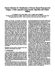
2.4.Experiment ExperimentDescription Description 2.4. Theexperiment experimentfor forthe theclassification classificationof ofhyperspectral hyperspectralimages imageswas wasimplemented implementedon onaaPHI PHIimage image The and an AVIRIS image. The airborne hyperspectral image collected by PHI covers the Fanglu Tea and an AVIRIS image. The airborne hyperspectral image collected by PHI covers the Fanglu Tea ◦ 0 00 ◦ 0 00 plantationarea areaininJiangsu Jiangsu province China, which is situated at (31 40N, 39119°22′53″ N, 119 22E).53WeE). We plantation province of of China, which is situated at (31°40′39″ used used an image with a size of 200 × 150 pixels and 65 spectral channels in the experiment. The image an image with a size of 200  150 pixels and 65 spectral channels in the experiment. The image was was collected on October Thecovered area where theimage imagecontains covers contains types ofcover, ground cover, collected on October 2002. 2002. The area by the 7 types of7 ground namely namelycaraway, paddy, caraway, wild-grass, pachyrhizus, tea, bamboo, and water. The spatial resolution of paddy, wild-grass, pachyrhizus, tea, bamboo, and water. The spatial resolution of the PHI the PHI image is 2 m. The AVIRIS image named Indian Pines covers the agricultural demonstration image is 2 m. The AVIRIS image named Indian Pines covers the agricultural demonstration zone in zone in Northwest of the Weanuse an image a size of 145 × 145 pixelsand and224 224spectral spectral Northwest Indiana Indiana of the US. WeUS. use image with with a size of 145 pixels  145 channels.ItItwas was collected collected on on June June 1992. 1992. The The area thebyimage coverscontains contains1616types typesofofground ground channels. area where covered the image cover, namely, alfalfa, corn-min (corn seeding), corn, grass/trees, grass/pasture, grass/pasture-moved cover, namely, alfalfa, corn-min (corn seeding), corn, grass/trees, grass/pasture, grass/pasture-moved (trimmed grass/pasture), grass/pasture),hay-windrowed, hay-windrowed,oats, oats,soybeans-notill soybeans-notill(no-till (no-tillsoybeans), soybeans),soybeans-min, soybeans-min, (trimmed soybean-clean (cleaned soybeans), wheat, woods, bldg-grass-tree-drives, stone-steel and soybean-clean (cleaned soybeans), wheat, woods, bldg-grass-tree-drives, stone-steel towerstowers and corncorn-notill. The spatial resolution of the AVIRIS image was 20 m. We used the AVIRIS image to notill. The spatial resolution of the AVIRIS image was 20 m. We used the AVIRIS image to test the test the feasibility ISBDD then the PHItoimage toapplicability test the applicability of ISBDD. feasibility of ISBDDofand thenand used theused PHI image test the of ISBDD. We call the hyperspectral image a data cube because it consists of two dimensions inthe thespatial spatial We call the hyperspectral image a data cube because it consists of two dimensions in dimension and one dimension in the spectral dimension. Figure 3 shows the data cube of the two dimension and one dimension in the spectral dimension. Figure 3 shows the data cube of the two imagescollected collectedby byAVIRIS AVIRISand andPHI, PHI,and andFigure Figure44shows showsthe thedistribution distributionof ofground groundcover coverin inthe thetwo two images images. Figure 4a is the ground truth image of the Indian Pines and Figure 4b is the ground survey images. Figure 4a is the ground truth image of the Indian Pines and Figure 4b is the ground survey imageof ofthe theFanglu FangluTea Tea plantation. plantation. The The two two images images can can describe describe the the distribution distribution of of ground ground cover cover.in In image Figure 4a, different color represents different types of ground cover, and the black color in the ground the two images. In Figure 4a, different colors represent different types of ground cover, and the black truth in image of Indiantruth Pinesimage represent area wherePines the ground coverareas is unknown. color the ground of the Indian represents where the ground cover is The spectral characteristic of seven types of ground cover in the Indian Pines are shown in unknown. Figure 5. The training and testing samples are selected from the image, and theirare specific information The spectral characteristic of seven types of ground cover in the Indian Pines shown in Figure is shown in Table 1. In this case, the training samples without interference for a certain type of ground 5. The training and testing samples are selected from the image, and their specific information is cover indicate that the labels of all pixels in the training samples are consistent with the label of shown in Table 1. In this case, the training samples without interference for a certain type of grounda certain type ofthat ground over. The samples with interference a certainwith classthe indicate that cover indicate the labels of alltraining pixels in the training samples arefor consistent label of a the training samples pixels whose labels are inconsistent with label of a certain type of certain type of groundcontain over. The training samples with interference for the a certain class indicate that

the training samples contain pixels whose labels are inconsistent with the label of a certain type of ground cover. In the stage of sample selection, we choose the pixels that have the inconsistent label as the interference for a type of ground cover. We choose interfered pixels and non-interfered pixels

Sensors 2018, 18, 780

6 of 14

ground cover. In the stage of sample selection, we choose the pixels which has the inconsistent label 6 of 14 as the interference for a type of ground cover. We choose pixels with interference and pixels without interference based on the ground image Pines of the and Indian andsurvey the ground image of the based on the ground truth image oftruth the Indian thePines ground imagesurvey of the Fanglu Tea Sensors 2017, 17, x FOR PEER REVIEW 6 of 14 Fanglu Tea plantation. Sensors 2017, 17, x FOR PEER REVIEW 6 of 14 plantation. Sensors 2017, 17, x FOR PEER REVIEW

based on ground the ground image of Indian the Indian Pines the ground survey image of Fanglu the Fanglu based on the truthtruth image of the Pines and and the ground survey image of the Tea Tea plantation. plantation.

Figure cube ofof images Figure3.3.Data Data cube imagescollected collectedbybyAVIRIS AVIRISand andPHI. PHI. Figure 3. Data of images collected by AVIRIS Figure 3. Data cubecube of images collected by AVIRIS and and PHI.PHI.

Figure 4. Distribution of ground coverininthe thetwo two images collected byby AVIRIS PHIPHI. Figure 4. Distribution ground cover images collected AVIRIS and Figure Distribution ofofground ground cover two images collected by AVIRIS and and PHI Figure 4. 4. Distribution of coverininthe the two images collected by AVIRIS and PHI

Figure 5. Spectral characteristic 16types types ofground ground covers covered inIndian thethe Indian Pines. Figure 5. characteristic 16 of covers covered in Indian Pines. Figure 5. Spectral Spectral characteristic of of 16of types of ground covers covered in the Pines.

Figure 5. Spectral characteristic of 16 types of ground covers covered in the Indian Pines.

Sensors 2017, 17, x FOR PEER REVIEW

7 of 14

Sensors 2018, 18, 780

7 of 14

Table 1. Number of training samples and testing samples for the Indian Pines.

Class ID

Training Samples Table 1. Number of training samples and testing samples for the Indian Pines.

1 2 31 42 53 64 5 76 87 98 9 10 10 11 11 12 12 13 13 14 14 15 15 16 16

Class ID

Testing Without Interference With Interference Samples Training Samples Alfalfa 25 32 18 Testing Samples Class Name Corn-min 28 35 81 Without Interference With Interference Corn 30 38 54 Alfalfa 25 32 18 Grass/trees 40 161 Corn-min 28 31 35 81 Corn 30 38 54 Grass/pasture 25 30 80 Grass/trees 31 20 40 16112 Grass/pasture-moved 25 Grass/pasture 25 30 80 Hay-windrowed 65 Grass/pasture-moved 20 50 25 1264 Oats 25 Hay-windrowed 50 20 65 6410 Oats 20 29 25 10 Soybeans-notill 37 155 Soybeans-notill 29 37 155 Soybeans-min 39 53 184 Soybeans-min 39 53 184 Soybean-clean 38 48 75 Soybean-clean 38 48 75 Wheat 30 40 Wheat 30 40 6060 Woods 48 156 Woods 38 38 48 156 Bldg-grass-tree-drives 30 30 25 6060 Bldg-grass-tree-drives 25 Stone-steel towers 35 45 16 Stone-steel towers 35 45 16 Corn-notill 30 38 178 Corn-notill 30 38 178 Class Name

Thespectral spectralcharacteristic characteristicofofthe theseven seventypes typesofofground groundcover coverininFanglu FangluTea Teaplantation plantationarea areaare are The shown in Figure 6. The training samples and testing samples are selected from the hyperspectral shown in Figure 6. The training samples and testing samples are selected from the hyperspectral image,and andthe thespecific specificinformation informationisisshown shownin inTable Table 2. 2. image,

Figure 6. Fanglu Tea plantation. Figure 6. Spectral Spectral characteristic characteristicof ofseven seventypes typesofofground groundcover covercovered coveredininthe the Fanglu Tea plantation.

Table and testing testing samples samples for for the the Fanglu Fanglu Tea Tea plantation. plantation. Table2.2.Number Number of of training training samples samples and Class Class ID ID 1(W2)

1(W2) 2(C4) 2(C4) 3(V13) 3(V13) 4(S2) 4(S2) 5(V2) 5(V2) 6(T7) 6(T7) 7(T6)

7(T6)

ClassName Name Class Water

Water Paddy Paddy Caraway Caraway Wild-grass Wild-grass Pachyrhizus Pachyrhizus Tea Tea Bamboo

Bamboo

Training Samples Testing Training Samples Testing Samples Samples Without Interference With Interference Without Interference With Interference 92 120 954 92 120 954 195 255 976976 195 255 105 138 295295 105 138 105 135 105 135 382382 66 82 66 82 211211 105 135 411 105 135 411443 135 180 135 180 443

Sensors 2018, 18, 780

8 of 14

The maximum likelihood (MLC) algorithm is a classical classification algorithm for remotely 2017, 17, x FOR PEER REVIEW 8 of 14 sensed Sensors images, and the support vector machine (SVM) method has been a popular and effective classification algorithm in recent years [22]. We compare the classifier based on MLC and SVM The maximum likelihood (MLC) algorithm is a classical classification algorithm for remotely algorithm with the classifier based on ISBDD algorithm. To fullyhas verify abilityand of the ISBDD sensed images, and the support vector machine (SVM) method been the a popular effective classifier, the DD classifier is utilized. The kernel function of the SVM classifier is the radial basis classification algorithm in recent years [22]. We compare the classifier based on MLC and SVM function. We select thethe tolerant penalty the SVMToclassifier. To verify the performance algorithm with classifier basedparameter on ISBDD of algorithm. fully verify the ability of the ISBDD of classifier, thepixels DD classifier is utilized. The kernel function of to thea SVM classifier the radial basisare the ISBDD model, with interference, which do not belong certain type ofisground cover, function. We select the tolerant penalty parameter of the SVM classifier. To verify the performance introduced to the training samples. Thereby, we use the training samples with interference to train of the ISBDD model, interfered pixels, which do without not belong to a certain are typea of ground cover, are the ISBDD and DD classifiers. The training samples interference subset of the training introduced to the training samples. Thereby, we use the training samples with interference to train samples. The MLC and SVM classifiers are applied to the hyperspectral image using the training the ISBDD and DD classifiers. The training samples without interference are a subset of the training samples without interference and the training samples with interference. samples. The MLC and SVM classifiers are applied to the hyperspectral image using the training The training samples of the two hyperspectral images are divided into five subsets, and the samples without interference and the training samples with interference. number of training samples in each subset equal. Five images roundsare of experiment and The training samples of the two is hyperspectral divided into are fiveconducted, subsets, and thethe final classification result issamples the average of the fiveisresults. The rounds design of of experiment a randomized experiment number of training in each subset equal. Five are block conducted, and can reduce the impact of random and avoid of the of results. The results the final classification result isfactors the average of the the five over-fitting results. The design a randomized blockare experiment theaccuracy, impact ofkappa random factors and avoid the over-fitting the results. The evaluated based oncan thereduce overall coefficient and accuracies of each of class. results are evaluated based on the overall accuracy, kappa coefficient and accuracies of each class.

3. Results 3. Results

3.1. AVIRIS Image 3.1. AVIRIS Image

We use the AVIRIS image to test the feasibility of ISBDD. Figure 7 shows the classified images of We useFigure the AVIRIS image to the feasibility of by ISBDD. Figureclassifiers, 7 shows the classified imagesDD the Indian Pines. 7a–f shows thetest images classified the MLC SVM classifiers, of the Indian Pines. Figure 7a–f shows the images classified by the MLC classifiers, SVM classifiers, and ISBDD classifiers. DD and ISBDD classifiers.

Figure 7. Classified images of the Indian Pines.

Figure 7. Classified images of the Indian Pines.

Sensors 2018, 18, 780

9 of 14

The classification performance can be measured by the classification accuracy of each type of ground cover, the overall accuracy, and the kappa coefficient. The classification accuracy of each type of ground cover can be used to evaluate the classification accuracy of each ground cover, and the overall accuracy can be used to evaluate the performance of a classifier on the entire image. The kappa coefficient can be used to evaluate the consistency of the classification results and the actual distribution. Table 3 shows the average classification accuracy comparison for the purpose of evaluating the performance of the four classifiers. The maximum accuracy is highlighted in bold. Table 3. Average classification accuracy comparison of the four classifiers. Method

MLC

SVM

MLC (Without Interference)

SVM (Without Interference)

DD

ISBDD

Alfalfa (%) Corn-min (%) Corn (%) Grass/trees (%) Grass/pasture (%) Grass/pasture-moved (%) Hay-windrowed (%) Oats (%) Soybeans-notill (%) Soybeans-min (%) Soybean-clean (%) Wheat (%) Woods (%) Bldg-grass-tree-drives (%) Stone-steel towers (%) Corn-notill (%) Overall accuracy (%) Kappa coefficient

85.56 56.22 97.14 60.40 81.00 63.33 99.87 24.00 32.39 78.16 100.0 95.67 98.10 11.00 100.0 40.95 68.17 0.65

100.0 67.55 98.57 75.30 100.0 100.0 90.67 92.00 57.32 88.78 100.0 100.0 99.05 34.33 100.0 35.81 77.74 0.76

81.11 66.71 97.14 79.06 87.17 11.67 99.87 8.00 28.31 88.57 100.00 97.33 98.33 7.33 100.00 18.86 69.92 0.67

100.00 96.22 98.57 99.73 100.00 100.00 89.87 100.00 56.34 85.30 100.00 100.00 99.29 39.67 98.40 47.43 84.75 0.84

100.0 77.20 24.29 91.41 100.0 100.0 77.74 88.00 77.32 77.96 93.21 100.0 93.33 50.67 29.60 60.57 80.55 0.79

100.0 91.19 75.71 95.70 100.0 100.0 89.87 100.0 76.62 94.90 100.0 100.0 100.0 59.00 99.20 65.52 89.02 0.88

Figure 7 and Table 3 show that the DD and ISBDD classifiers perform better than the MLC and SVM classifiers when the training samples contain interference. The ISBDD classifier performs best in the classification accuracy of each type of ground cover because it has the highest classification accuracy in 10 of the 16 types of ground cover. The capacity of the DD and ISBDD classifiers to deal with the interference problem benefits from their MIL framework. The ISBDD classifier performs better than the MLC and SVM classifiers even if its training samples contain interference, whereas the training samples of the MLC and SVM classifiers do not contain interference. However, the DD classifier is not effective in this situation because the ISBDD classifier employs a novel training strategy in the training process. The result proves that the use of ISBDD is feasible for handling the interference problem. 3.2. PHI Image We use the AVIRIS image to test the applicability of ISBDD. The classified images of the Fanglu tea plantation are shown in Figure 8. Figure 8a–f shows the images classified by the four classifiers.

Sensors 2018, 18, 780 Sensors 2017, 17, x FOR PEER REVIEW

10 of 14 10 of 14

Figure8.8.Classified Classifiedimages imagesofofthe theFanglu FangluTea Tea plantation. Figure plantation.

Table 4 shows the average classification accuracy comparison for the purpose of evaluating the Table 4 shows the average classification accuracy comparison for the purpose of evaluating the performance of the four classifiers. The maximum precision is highlighted in bold. performance of the four classifiers. The maximum precision is highlighted in bold. Table 4. Average classification accuracy comparison of the four classifiers. Table 4. Average classification accuracy comparison of the four classifiers.

Method

Method

Water (%)

Water (%) Paddy Paddy (%)(%) Caraway (%) (%) Caraway Wild-grass (%) Wild-grass Pachyrhizus (%)(%) Tea (%) Pachyrhizus (%) Bamboo (%) Tea (%)(%) Overall accuracy Kappa coefficient Bamboo (%)

MLC

MLC

92.24

92.24 69.45 69.45 98.37 98.37 79.58 79.58 88.72 95.08 88.72 94.40 95.08 85.74 0.83 94.40

MLC (Without MLC (Without SVM Interference) Interference) 95.66 91.72

SVM

95.66 80.00 80.00 98.10 98.10 72.09 72.09 90.05 97.13 90.05 96.61 97.13 89.20 0.87 96.61

91.72 82.09 82.09 100.00 100.00 92.98 92.98 96.97 98.30 96.97 90.52 98.30 90.85 0.89 90.52

SVM (Without SVM (Without Interference) Interference)

94.32

94.32 98.07 98.07 99.46 99.46 94.56 94.56 97.91 98.74 97.91 92.69 98.74 96.26 0.95 92.69

DD

DD

93.27

93.27 71.74 71.74 99.52 99.52 96.65 96.65 96.78 99.37 96.78 94.72 99.37 89.46 0.87 94.72

ISBDD ISBDD

97.72

97.72 99.78 99.78 98.85 98.85 92.20 92.20 95.26 98.73 95.26 96.89 98.73 97.65 0.97 96.89

97.65 Overall accuracy (%) 85.74 89.20 90.85 96.26 89.46 0.97 the Kappa coefficient 0.95SVM is the0.87 Figure 8 and Table 4 show0.83 that the0.87 classification0.89 accuracy of MLC and lowest when training samples contain interference. However, when the training samples are pure, the classification Figure 8 and Table 4 show that the classification accuracy of MLC and SVM is the lowest accuracy of these classifiers is high, especially for the SVM. The ISBDD classifier performs best inwhen the the trainingaccuracy samplesofcontain interference. However, when samples are accuracy pure, the classification each type of ground cover because it hasthe thetraining highest classification accuracy classifiers is high, the SVM. The inclassification three of the seven typesofofthese ground cover. The overallespecially accuracy for of ISBDD is also theISBDD highest,classifier while performs best inaccuracy the classification of that eachoftype ground coverinterference). because it hasThe theresults highest the classification of DD is accuracy lower than the of SVM (without classification accuracy in three of the seven types of ground cover. The overall accuracy of ISBDD is demonstrate the effectiveness of ISBDD. alsoThe the classification highest, while the classification of DDimages is lower than that of SVM (without results of the two accuracy hyperspectral demonstrate thethefeasibility and interference). results model demonstrate the training effectiveness of ISBDD. applicability of The the ISBDD when the samples contain interference. When the training The classification results of the two hyperspectral images demonstrate the feasibility and applicability of the ISBDD model when the training samples contain interference. When the training

Sensors 2018, 18, 780 Sensors 2017, 17, x FOR PEER REVIEW

11 of 14 11 of 14

samples do not contain interference, the MLC classifier and the SVM classifier can achieve samples are not contain interference, the MLC classifier and the SVM classifier can achieve satisfactory satisfactory classification accuracy. However, when the training samples contain interference, the classification accuracy. However, when the training samples contain interference, the advantage of the advantage of the ISBDD model is apparent. ISBDD model is apparent. 4.4.Discussion Discussion 4.1. 4.1.Influence InfluenceofofInterference InterferenceIntensity Intensity The Thepurpose purposeofofthe theDD DDand andISBDD ISBDDmodel modelisisto todeal dealwith withproblem problemof ofinterference, interference,wherein whereinthe the proportion of interfered pixels can modulate the performance of the classifiers. Figure 9 shows the proportion of pixels with interference can modulate the performance of the classifiers. Figure 9 shows impact of theof proportion of interfered pixels in interference the training samples on classification using the impact the proportion of pixels with in the training samples accuracies on classification the four classifiers forfour the Indian Pines The x-axis is the ratio interfered to pixels nonaccuracies using the classifiers forimage. the Indian Pines image. Theofx-axis is the pixels ratio of interfered pixels in the training samples, indicating the intensity of interference. The y-axis shows the with interference to pixels without interference in the training samples, indicating the intensity of overall accuracy. interference. The y-axis shows the overall accuracy.

Figure 9. The of intensity of interference on classification accuracy for the Pines.Pines. Figure 9. impact The impact of intensity of interference on classification accuracy for Indian the Indian

Figure 9 shows that the overall accuracy of the ISBDD classifier is higher than that of the other Figure 9 shows that the overall accuracy of the ISBDD classifier is higher than that of the other classifiers. In cases where the ratio is larger than 0.5, the overall accuracy of the MLC and SVM classifiers. In cases where the ratio is larger than 0.5, the overall accuracy of the MLC and SVM classifier declines sharply, whereas the overall accuracy of the DD and ISBDD classifier declines classifier declines sharply, whereas the overall accuracy of the DD and ISBDD classifier declines slowly. slowly. However, the decline range of overall accuracy from 0 to 0.9 of the ISBDD classifier is almost However, the decline range of overall accuracy from 0 to 0.9 of the ISBDD classifier is almost the same the same as that of the MLC classifier, and these results demonstrate the advantage of ISBDD in as that of the MLC classifier, and these results demonstrate the advantage of ISBDD in dealing with dealing with the interference problem. the interference problem. Figure 10 illustrates the impact of the intensity of interfered pixels in training samples on Figure 10 illustrates the impact of the intensity of pixels with interference in training samples classification accuracy when the four classifiers are used for the Indian Pines image. The x-axis shows on classification accuracy when the four classifiers are used for the Indian Pines image. The x-axis the ratio of the interfered pixels to non-interfered pixels in the training samples. The y-axis shows the shows the ratio of the pixels with interference to pixels without interference in the training samples. overall accuracy. The y-axis shows the overall accuracy. Figure 10 shows that the overall accuracy of the ISBDD classifier is higher than that of the other Figure 10 shows that the overall accuracy of the ISBDD classifier is higher than that of the other classifiers. The DD classifier does not perform better than the SVM or the MLC classifier when the classifiers. The DD classifier does not perform better than the SVM or the MLC classifier when the ratio of interfered pixels and non-interfered pixels is smaller than 0.2. However, when the ratio is ratio of pixels with interference and pixels without interference is smaller than 0.2. However, when the larger than 0.4, the overall accuracy of the MLC and SVM classifier declines sharply, whereas the ratio is larger than 0.4, the overall accuracy of the MLC and SVM classifier declines sharply, whereas overall accuracy of the DD and ISBDD classifier declines slowly. The result shows that the MLC the overall accuracy of the DD and ISBDD classifier declines slowly. The result shows that the MLC classifier and the SVM classifier is more sensitive to interference than the ISBDD classifier. classifier and the SVM classifier is more sensitive to interference than the ISBDD classifier.

Sensors 2018, 18, 780 Sensors 2017, 17, x FOR PEER REVIEW

12 of 14 12 of 14

Figure 10. The impact of intensity of interference on classification accuracy for the Fanglu tea Figure 10. The impact of intensity of interference on classification accuracy for the Fanglu tea plantation. plantation.

4.2. Application Prospects and Future Work 4.2. Application Prospects and Future Work An increasing number of satellites equipped with hyperspectral camera are being launched for An increasing number of satellites equipped with hyperspectral camera are being launched for the purpose of crop survey, military target detection, and so on. The research and application of the purpose of crop survey, military target detection, and so on. The research and application of pattern recognition, such as face detection, is also gaining popularity. All these fields are concerned pattern recognition, such as face detection, is also gaining popularity. All these fields are concerned with supervised classification, in which the interference problem is inevitable when selecting the with supervised classification, in which the interference problem is inevitable when selecting the training samples. The ISBDD can be used in supervised classification to handle the problem of training training samples. The ISBDD can be used in supervised classification to handle the problem of samples with interference. The training strategy of ISBDD provides the model the powerful capability interfered training samples. The training strategy of ISBDD provides the model the powerful to complete the classification task though the training samples that contain interference. capability to complete the classification task though the training samples that contain interference. However, the high accuracy cost of the ISBDD classifier is that its computational complexity is However, the high accuracy cost of the ISBDD classifier is that its computational complexity is higher than that of the DD classifier. Suppose that w is the width of a hyperspectral image, and h is higher than that of the DD classifier. Suppose that w is the width of a hyperspectral image, and h is the height of a hyperspectral image, then the w × h pixels exist completely in the hyperspectral image. the height of a hyperspectral image, then the w h pixels exist completely in the hyperspectral Assuming that a total of N pixels exist in the positive bags and the image contains c types of ground image. Assuming that a total of N pixels exist in the positive bags and the image contains c types of cover, then in the training process, most computing resources are used to determine the DD value. ground cover, then in the training process, most computing resources are used to determine the DD Thus, the ratio of the computational complexity of the ISBDD classifier to that of the DD classifier can value. Thus, the ratio of the computational complexity of the ISBDD classifier to that of the DD be described as follows: classifier can be described as follows: w×h×c R= (10) w hN c (10) R In general, the numerator of Formula (10)N is greater than the denominator. Thus, the computational of the ISBDD classifier considerably higher. efficiency ofThus, the ISBDD In general,complexity the numerator of Formula (10)is is greater than the The denominator. the classifier should be improved because, in many situations, efficiency is crucial. One of the solutions for computational complexity of the ISBDD classifier is considerably higher. The efficiency of the ISBDD improving efficiency is to utilize the multi-thread technique and parallel computing, given that the classifier should be improved because, in many situations, efficiency is crucial. One of the solutions computing process for each pixel in the ISBDD classifier is independent. for improving efficiency is to utilize the multi-thread technique and parallel computing, given that

the computing process for each pixel in the ISBDD classifier is independent. 5. Conclusions 5. Conclusions The ISBDD model, which employs a novel training strategy, is proposed in this paper. The major contribution of this work is in exploring a model with high classification accuracy to handle The ISBDD model, which employs a novel training strategy, is proposed in this paper. The major the problem of training samples with interference in the classification of hyperspectral image. In contribution of this work is in exploring a model with high classification accuracy to handle the the proposed model, instead of learning a feature vector to represent the training bags, pixels are problem of interfered training samples in the classification of hyperspectral image. In the proposed classified directly according to training bags. The ISBDD model is compared with several classical model, instead of learning a feature vector to represent the training bags, pixels are classified directly hyperspectral image classification models, including the diverse density model. Results demonstrated according to training bags. The ISBDD model is compared with several classical hyperspectral image that the classifier based on the ISBDD model performs better than that based on other algorithms. classification models, including the diverse density model. Results demonstrated that the classifier based on the ISBDD model performs better than that based on other algorithms. Specifically, the

Sensors 2018, 18, 780

13 of 14

Specifically, the overall accuracy of the ISBDD classifier is approximately 8% higher than that of the DD classifier. The overall accuracy of the proposed classifier is much higher than the SVM and MLC classifiers when the training samples contain interference. The results show that the ISBDD classifier can handle the interference problem effectively. In addition, it can be used in classification scenarios, especially when an accurate classification is highly required. However, the computational complexity of the ISBDD model is higher than that of the DD classifier because several DD values are computed for each pixel. Thus, the multi-thread technique and parallel computing can be utilized to increase the efficiency. Acknowledgments: This work was supported by the National High Technology Research and Development Program (863 Program) (Grant No. 2012YQ05250 and No. 2016YFF0103604), National Key Technologies R&D Program (Grant No. 2016YFB0500505), National Natural Science Foundation of China (Grant No. 41402293), Program for Changjiang Scholars and Innovative Research Team (Grant No. IRT0705), China Scholarship Council (Ref No. 201606025034) and the UK Science and Technology Facilities Council (STFC) through the PAFiC project (Ref: ST/N006801/1). Author Contributions: Na Li and Huijie Zhao conceived and designed the algorithm; Zhaopeng Xu and Xinchen Huang performed the experiments; Na Li and Zhaopeng Xu analyzed the results; Zhenhong Li, Jane Drummond and Daming Wang provided comments on the algorithm and experiments. Conflicts of Interest: The authors declare no conflict of interest.

References 1.

2.

3. 4. 5. 6. 7. 8.

9. 10. 11. 12. 13.

14.

Garaba, S.P.; Zielinski, O. Comparison of remote sensing reflectance from above-water and in-water measurements west of Greenland, Labrador Sea, Denmark Strait, and west of Iceland. Opt. Express 2013, 21, 15938–15950. [CrossRef] [PubMed] Filippi, A.M.; Archibald, R.; Bhaduri, B.L.; Bright, E.A. Hyperspectral agricultural mapping using support vector machine-based endmember extraction (SVM-BEE). Opt. Express 2009, 17, 23823–23842. [CrossRef] [PubMed] Babaeian, E.; Homaee, M.; Montzka, C.; Vereecken, H.; Norouzi, A.A. Towards retrieving soil hydraulic properties by hyperspectral remote sensing. Vadose Zone J. 2015, 14. [CrossRef] Klein, M.E.; Aalderink, B.J.; Padoan, R.; De Bruin, G.; Steemers, T.A. Quantitativen Hyperspectral Reflectance Imaging. Sensors 2008, 8, 5576–5618. [CrossRef] [PubMed] Jia, X.; Kuo, B.C.; Crawford, M.M. Feature mining for hyperspectral image classification. Proc. IEEE 2013, 101, 676–697. [CrossRef] Qi, B.; Zhao, C.; Youn, E.; Nansen, C. Use of weighting algorithms to improve traditional support vector machine based classifications of reflectance data. Opt. Express 2011, 19, 26816–26826. [CrossRef] [PubMed] Li, N.; Cao, Y. An improved classification approach based on spatial and spectral features for hyperspectral data. Spectrosc. Spectr. Anal. 2014, 34, 526–531. Li, N.; Zhao, H.J.; Huang, P.; Jia, G.R.; Bai, X. A novel logistic multi-Class supervised classification model based on multi-fractal spectrum parameters for hyperspectral Data. Int. J. Comput. Math. 2015, 92, 836–849. [CrossRef] Tao, D.; Jia, G.; Yuan, Y.; Zhao, H. A digital sensor simulator of the pushbroom offner hyperspectral imaging spectrometer. Sensors 2014, 14, 23822–23842. [CrossRef] [PubMed] Dietterich, T.G.; Lathrop, R.H.; Lozano-Pérez, T. Solving the multiple instance problem with axis-parallel rectangles. Artif. Intell. 1997, 89, 31–71. [CrossRef] Maron, O.; Lozano-Pérez, T. A framework for multiple-instance learning. Adv. Neural Inf. Process. Syst. 1998, 200, 570–576. Du, P.; Samat, A. Multiple instance learning method for high-resolution remote sensing image classification. Remote Sens. Inf. 2012, 27, 60–66. Wada, T.; Mukai, Y. Fast Keypoint Reduction for Image Retrieval by Accelerated Diverse Density Computation. In Proceedings of the 2015 IEEE International Conference on Data Mining Workshop, Atlantic City, NJ, USA, 14–17 November 2015; pp. 102–107. Bolton, J.; Gader, P. Application of Multiple-Instance Learning for Hyperspectral Image Analysis. IEEE Geosci. Remote Sens. Lett. 2015, 8, 889–893. [CrossRef]

Sensors 2018, 18, 780

15.

16.

17. 18.

19.

20. 21. 22.

14 of 14

Bolton, J.; Gader, P. Multiple instance learning for hyperspectral image analysis. In Proceedings of the 2010 IEEE International Geoscience and Remote Sensing Symposium (IGARSS), Honolulu, HI, USA, 25–30 July 2010; pp. 4232–4235. Bolton, J.; Gader, P. Spatial multiple instance learning for hyperspectral image analysis. In Proceedings of the 2010 2nd Workshop on Hyperspectral Image and Signal Processing: Evolution in Remote Sensing, Reykjavik, Iceland, 14–16 June 2010; Volume 8, pp. 1–4. Vanwinckelen, G.; Fierens, D.; Blockeel, H. Instance-level accuracy versus bag-level accuracy in multi-instance learning. Data Min. Knowl. Discov. 2016, 30, 313–341. [CrossRef] Xu, L.; Guo, M.Z.; Zou, Q.; Liu, Y.; Li, H.F. An Improved Diverse Density Algorithm for Multiple Overlapped Instances. In Proceedings of the Fourth International Conference on Natural Computation (ICNC ’08), Jinan, China, 18–20 October 2008. Fu, J.; Yin, J. Bag-level active multi-instance learning. In Proceedings of the Eighth International Conference on Fuzzy Systems and Knowledge Discovery (FSKD), Shanghai, China, 26–28 July 2011; Volume 2, pp. 1307–1311. Chen, M.S.; Yang, S.Y.; Zhao, Z.J.; Fu, P.; Sun, Y.; Li, X.; Sun, Y.; Qi, X. Multi-points diverse density learning algorithm and its application in image retrieval. J. Jilin Univ. 2011, 41, 1456–1460. Ordóñez, C.; Cabo, C.; Sanz-Ablanedo, E. Automatic Detection and Classification of Pole-Like Objects for Urban Cartography Using Mobile Laser Scanning Data. Sensors 2017, 17, 1465. [CrossRef] [PubMed] Kozoderov, V.V.; Dmitriev, E.V. Testing different classification methods in airborne hyperspectral imagery processing. Opt. Express 2016, 24, A956–A965. [CrossRef] [PubMed] © 2018 by the authors. Licensee MDPI, Basel, Switzerland. This article is an open access article distributed under the terms and conditions of the Creative Commons Attribution (CC BY) license (http://creativecommons.org/licenses/by/4.0/).