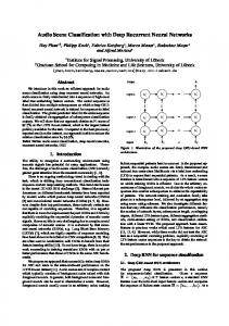
Training Small Networks for Scene Classification of Remote ... - MDPI
Recommend Documents
Apr 6, 2016 - automotive scenarios where labelled data is similarly scarce or ... for rarer but important classes such as pedestrians and cyclists, which can ...
Apr 6, 2016 - automotive scenarios where labelled data is similarly scarce or fragmented and ... for rarer but important classes such as pedestrians and cyclists, ...... Vision-based offline-online perception paradigm for autonomous driving.
Scene Classification via Triplet Networks. Yishu Liu and Chao Huang. AbstractâScene classification is a fundamental task for auto- matic remote sensing image ...
Mar 2, 2017 - Scene Classification with General Features Learned ... of benchmarks[15â18]. .... information and test its performance for different remote sensing .... By integrating the two directions discussed above, deep residual network (ResNet)
Email: [email protected], [email protected]. Telephone: +358-8-533 2796, Fax: +358-8-533 2796. AbstractâClassification of textures in scene images is very.
Mar 5, 2018 - Flow chart of the DD and ISBDD models. 2.4. ..... Filippi, A.M.; Archibald, R.; Bhaduri, B.L.; Bright, E.A. Hyperspectral agricultural mapping using ...
propose a partial discriminative training (PDT) scheme for neural net- works .... generally transformed to multiple binary classification tasks, and different meth-.
May 4, 2018 - a supervised classification method that is based on an interval type-2 .... Gaussian mixture models (GMM) of the training samples, is used for ...
Our proposal is to use a classification system based on features extracted from the ..... explained based on the existence of evidence of ticket of the projectile for ...
This paper discusses two novel artificial neural network architectures applied to ... These approaches are 1) a spiking-neural-network model for the partitioning ...
97.7% on the LITIS Rouen dataset, which is the largest dataset publicly available for ... Index Terms: audio scene classification, deep neural networks, recurrent ...
Mar 14, 2017 - gained great attention of the research community [1, 2]. There is an ..... [17] A. Graves, A. rahman Mohamed, and G. Hinton, âSpeech recogni-.
Mar 14, 2018 - where the minimum internal difference, MInt(C1, C2), is defined as ..... car class is the lowest due to cars containing fewer pixels, easily leading ...
May 7, 2013 - Depth maps are crucial for three-dimensional (3D) imaging and display, which have ... In addition, with the development of distributed networks, remote monitoring and ... compressed and transmitted to the terminal side for dynamic 2D ..
Nov 11, 2013 - Smeeckaert, J., Mallet, C., David, N., Chehata, N., Ferraz, A.,. Large-scale water classification of coastal areas using airborne topographic lidar ...
Remote Sensing Scene Classification and Explanation ... - MDPI › publication › fulltext › Remote-S... › publication › fulltext › Remote-S...by SC Hung · 2020 · Cited by 2 · Related articlesSep 4, 2020 — Example images of RSSCN7 dataset: (a) grass;
Learning a Kernel Function for Classification with Small Training Samples. Tomer Hertz. [email protected]. Aharon Bar
be referred to as Window Resizing and abbreviated as WR. We .... âall historyâ and is abbreviated as ALL. .... Machine Intelligence, 11(10):1087â1101, 1989.
A training data selection method for multi-class data is proposed. This method ... 1. 1 + exp(ânetk). (3). To train the MLNN, Back-propagation algorithm is used.
Mar 18, 2016 - This paper develops a supervised collaborative kernel coding .... based on the dictionary coefficients and learned linear classifier, a label ...
digital cameras, camcorders, mobile phones with built-in cameras; and storage of personal ... semantic concept in this method as it uses only the counts of visual words ... representation scheme for the images and it is compulsory for initializing.
supported for programming languages such as C, C++, and Java, used for the 3D object ... horizontal and the vertical axi
Project page and open source code: http://cvjena.github.io/cn24/. Abstract. In this paper, we present convolutional patch networks, .... as a directed graph.
Training Small Networks for Scene Classification of Remote ... - MDPI
May 7, 2018 - Features extracted by methods are utilized to train shallow classifiers such as Support ... To improve the classification accuracy, various low-level local descriptors ... Most are based on deep convolutional neural network (CNN) models, such as ...... Liu, Y.; Huang, C. Scene classification via triplet networks.
remote sensing Article
Training Small Networks for Scene Classification of Remote Sensing Images via Knowledge Distillation Guanzhou Chen ID , Xiaodong Zhang *, Xiaoliang Tan, Yufeng Cheng Yuanfu Gong and Qing Wang
Abstract: Scene classification, aiming to identify the land-cover categories of remotely sensed image patches, is now a fundamental task in the remote sensing image analysis field. Deep-learning-model-based algorithms are widely applied in scene classification and achieve remarkable performance, but these high-level methods are computationally expensive and time-consuming. Consequently in this paper, we introduce a knowledge distillation framework, currently a mainstream model compression method, into remote sensing scene classification to improve the performance of smaller and shallower network models. Our knowledge distillation training method makes the high-temperature softmax output of a small and shallow student model match the large and deep teacher model. In our experiments, we evaluate knowledge distillation training method for remote sensing scene classification on four public datasets: AID dataset, UCMerced dataset, NWPU-RESISC dataset, and EuroSAT dataset. Results show that our proposed training method was effective and increased overall accuracy (3% in AID experiments, 5% in UCMerced experiments, 1% in NWPU-RESISC and EuroSAT experiments) for small and shallow models. We further explored the performance of the student model on small and unbalanced datasets. Our findings indicate that knowledge distillation can improve the performance of small network models on datasets with lower spatial resolution images, numerous categories, as well as fewer training samples. Keywords: knowledge distillation; scene classification; convolutional neural networks (CNNs); remote sensing; deep learning
1. Introduction With the rapid development of remote sensing (RS) techniques, a large number of algorithms have been proposed to automatically process massive earth observation data. Scene classification is the one of fundamental procedures of RS images analysis and of much importance in many RS applications, such as land-use/land-cover (LULC) [1–4], agriculture [5–8], forestry [9,10], and hydrology [11]. The core task of scene classification is to identify the land-cover type of remotely sensed image patches automatically. Numerous supervised machine learning algorithms have been used in scene classification. These algorithms can be categorized into the following three types [12]: low-level, mid-level and high-level methods. Low-level methods first extract low-level hand-crafted features, including SIFT (scale invariant feature transform) [13,14], HOG (histogram of oriented gradients) [15], structural texture similarity [16], LBP (local binary patterns) [17], Gabor descriptors [18], etc. Features extracted by methods are utilized to train shallow classifiers such as Support Vector Remote Sens. 2018, 10, 719; doi:10.3390/rs10050719
www.mdpi.com/journal/remotesensing
Remote Sens. 2018, 10, 719
2 of 20
Machines (SVMs) [19] or K-Nearest Neighbor algorithms (KNNs) [20] to identify the categories of scene images. These scene classification methods based on low-level features are efficient on some structures and arrangements, but cannot easily depict the highly diverse and non-homogeneous spatial distributions in images [21].Mid-level methods build scene representations by coding low-level local attributes. The bag-of-visual-words (BoVW) model is one of the most frequently used approaches [22]. To improve the classification accuracy, various low-level local descriptors are combined as complemented features in the standard BoVW model [23], Gaussian mixture model (GMM) [24], and other pyramid-based models [25–27] for scene classification. In addition, topic models are introduced to combine visual semantic information to encode higher order spatial information between low-level local visual words [28–32]. High-level methods are based on deep learning (DL) models. DL models achieve the state-of-the-art in image recognition, speech recognition, semantic segmentation, object detection, natural language processing [33–36], and RS image scene classification. Many classic DL models in the field of computer vision (CV) have been shown to be effective in RS scene classification [12,37–44]. Most are based on deep convolutional neural network (CNN) models, such as AlexNet [45], CaffeNet [46], VGGNet [47], deep residual networks (ResNet) [48] and DenseNets [49]. Among these approaches, the CNN-based high-level models outperform the state-of-the-art for scene classification tasks in remote sensing [50]. They can deal with scenes that are more complex and achieve higher overall accuracy by learning deep visual features from large training datasets, in contrast to shallow models and low-level methods that rely on manual feature extraction [51]. However, deep CNNs contain more parameters to train, thus they cost more computational resources and time on training and predicting. For example, a 102-convolutional-layer CNN model, which contains 42.4 M parameters, costs 14 ms to classify a 224 × 224 × 3 scene image while a simple 4-convolutional-layer CNN model costs 8.77 ms and only contains 1 M parameters, as detailed in Section 3.1 of this paper. This is an unacceptable cost of time and storage space in special situations, such as embedded devices [52–54] or during on-orbit processing [55]. In contrast, a small and shallow model is fast and uses little space, but will not yield accurate and precise results when trained directly on ground truth data [33]. Under these circumstances, model compression techniques become imperative. Generalized model compression improves the performance of a shallow and fast model by learning a cumbersome, but better performing model, or by simplifying the structure of the cumbersome network. There are three mainstream types of model compression algorithms: network pruning, network quantization and Teacher-Student Training (TST). Network pruning is a technique that reduces the size of networks by removing neurons or weights that are less important based on certain standard [52,56–58], while network quantization attempts to reduce the precision of weights or features [59–61]. In contrast, TST methods impart knowledge from a teacher model into a student model by learning distributions or outputs of some specific layers [62–70]. TST is easily confused with transfer learning. In transfer learning, we first train a base model on a certain dataset and task, and then transfer the learned features to another target network to be trained on different target dataset and task [71,72]. A common use of transfer learning in the field of remote sensing is to fine-tune an ImageNet-pretrained model on a remote sensing dataset [2,40,73]. In a TST process, however, the teacher and student models are trained on the same dataset. Knowledge distillation (KD) is one kind of TST method, first defined in [63]. In that paper, authors distill knowledge from an ensemble of models into a single smaller model via high-temperature softmax training. In this paper, we introduce the KD into remote sensing scene classification for the first time to improve the performance of small and shallow network model. We then conducted experiments on several public datasets to verify the effectiveness of KD and make a quantitative analysis to explore the optimum parameter settings. We will also discuss performance of KD on different types of datasets. In addition, we tested whether knowledge can still be distilled in the absence of a certain type of training samples or in the absence of sufficient training data sets. For convenience in our work, we simplified the KD training process by only learning from one cumbersome model. The rest of this
Remote Sens. 2018, 10, 719
3 of 20
paper is organized as follows. Section 2 will describe the teacher-student training method and our knowledge distillation framework. In Section 3, results and analysis of experiments on several datasets are detailed. Our conclusion and future work are discussed in Section 4. 2. Method As a special case of teacher-student training (TST), knowledge distillation (KD) imitates high-temperature softmax output from the cumbersome teacher model, serving as our training framework. In this section, we first describe the different TST methods, and introduce the KD training methods we adopted in our research. 2.1. Teacher-Student Training TST is one of the mainstream model compression methods. In TST processing, a cumbersome pre-trained model is regarded as a teacher, the untrained small and shallow model is a student. The student model not only learns hard target from the ground truth data, but also matches its output to the output of the teacher model. This is because the output of a softmax layer (soft target) contains more information than one-hot labeled dataset (hard target). A general TST process first trains the cumbersome model directly on dataset and then train the student model by minimizing the following loss function using mini-batch stochastic gradient descent (MSGD) [74] method: L TST ( X ) = λ · H1 (S( X ), YGT ) + H2 (S∗ ( X ), T ∗ ( X ))
(1)
where X denotes a batch of input data, S( X ) is the softmax output of student model, YGT is the ground truth label corresponding to the input X, and S∗ ( X ) and T ∗ ( X ) are the output of a certain layer in student model and teacher model, λ is a non-negative constant. The first term in this loss function is a ground truth constraint. If λ = 0, the supervised information is only provided by the teacher model, instead of the ground truth data. If λ goes higher, the output probability distribution of the trained student model is more like the teacher model. H1 ( X,Y ) and H2 ( X,Y ) in Equation (1) can be any common loss functions, such as mean squared error (MSE) or categorical crossentropy (CE):
CE( x, y) = −
1 m
1 m
m
d
∑ ∑ (xik − yik )2
(2)
∑ ∑ [xik log (yik ) + (1 − xik ) log (1 − yik )]
(3)
MSE( x, y) = m
i =1 k =1
d
i =1 k =1
where m denotes the batch size, d denotes the size of input vector x, and xik indicates the kth element of the ith input samples. The simplest and the naive method in TST matches the output probability distribution of the last softmax layer (MS) in the student model to the teacher model. In this case, S∗ ( X ) = S( X ) and T ∗ ( X ) is the softmax output of the teacher model. Thus, the loss function of MS mode can be defined as: L MS ( X ) = λ · CE(S( X ), YGT ) + CE(S( X ), T ( X ))
(4)
To better impart knowledge from teacher to student, Bucilua, C., et al. [62] proposed the matching logits (ML) method. Logits are the inputs to the final softmax layer of a network. Here, the discrepancy among categories in the logits form is more significant than the probabilities form. As a result, the CE of the second term in the loss function are replaced by MSE because the value of a logit can be any real number. The loss function in ML mode now becomes: L ML ( X ) = λ · CE(S( X ), YGT ) + MSE(Slogits ( X ), Tlogits ( X ))
(5)
Remote Sens. 2018, 10, 719
4 of 20
where Slogits ( X ) and Tlogits ( X ) are the logits output of their model. In that work, the authors conducted several experiments and verified that the ML mode could improve small models by learning from model ensembles in simple machine learning tasks. In addition to these methods as mentioned, various researchers in the field have proposed other means for TST training. Huang, Z., et al. [69] proposed an idea of matching the distributions of neuron selectivity patterns (NST) between two networks, where a new loss function through minimizing the maximum mean discrepancy (MMD) is designed to match these distributions. In [70], the authors compressed wide and shallow networks into thin but deeper networks, the FitNet, by learning intermediate-level hints from teacher’s hidden layers. Yim [68] transfers the knowledge distilled from the flow between layers, computed by the inner product between features, and generated into the FSP matrix. Different from the previous methods, Chen, T., et al. [64] accelerates the training of a larger network by transferring knowledge from a network to the new larger network. Lopez-Paz, D., et al. [66] combines knowledge distillation with privileged information [75], deriving into a generalized distillation. 2.2. Knowledge Distillation Framework 2.2.1. Knowledge from Probability Distribution The last output layer of neural networks is the softmax layer that transforms the logits zi into a probability pi via: pi = so f tmax (zi ) =
exp(zi ) ∑ j exp(z j )
(6)
However, the normal softmax output always leads to an approximate one-hot vector. An example is shown in Table 1 and Figure 1, which indicates that normal softmax (temperature = 1) made the probability of C2 class tends to one and others tend to zero. The entropy of the output also tends to zero. In practice, a remote sensing scene image consists of several categories of pixels. Thus, information for non-maximum probability categories provides additional supervision for training. 1.0 0.9 0.8 0.7 0.6 0.5 0.4 0.3 0.2 0.1 0.0
T=1
T=100 C1
C2
T=200 C3
C4
C5
T=500
C6
Figure 1. An example of categorical probability distributions of high-temperature softmax output with different temperature. C1∼C6 denote six categories. The input logit data are listed in the last row of Table 1. When T = 1 (normal softmax), the probability of C2 tends to 1 and others tend to 0. If T goes higher, the categorical distribution tends to be more consistent.
Remote Sens. 2018, 10, 719
5 of 20
Table 1. An example of high-temperature softmax output with different temperature. Temperature
C1
C2
C3
C4
C5
C6
Entropy 1
1 100 200 500
0.0000 0.0523 0.1338 0.1687
1.0000 0.8566 0.5416 0.2951
0.0000 0.0022 0.0275 0.0896
0.0000 0.0320 0.1046 0.1529
0.0000 0.0160 0.0741 0.1331
0.0000 0.0409 0.1183 0.1606
0.0000 0.8764 1.9934 2.4898
logits
−304.63
−25.01
−620.91
−353.81
−422.91
−329.22
1
Log2-based entropy.
To improve the discrimination ability and generalizability of a model, Hinton, G., et al. [63] introduced high temperature softmax function instead of normal softmax or logits. High temperature softmax function was first used in the field of reinforcement learning [76], denoted as: pi =
exp(zi /T ) ∑ j exp(z j /T )
(7)
where T is the temperature. The normal softmax is a special case if T = 1. Softmax with high temperature could increase the entropy of the categorical vector which helps to learn more knowledge from the probability distribution of a complex scene. An example of categorical probability distributions of high-temperature softmax output with different temperature is shown in Table 1 and Figure 1. C1∼C6 denote six categories, and the example input logit data are listed in the last row of the table. When T = 1 (normal softmax), the probability of C2 tends to 1 and others tend to 0. If T goes higher, the entropy of the categorical distribution becomes higher. It can be inferred from this example that if the student model learns high-temperature softmax output from the teacher model, it will distill more knowledge of categorical probability distribution. The experiments in Section 3 will verify this inference. 2.2.2. KD Training Process By introducing the high-temperature softmax into our framework in former subsection, we divide the whole training process of knowledge distillation into two procedures. First, train the teacher model directly on dataset, which is shown in Figure 2a. The target is to let T ( X ), the softmax output of the teacher model, fit the ground truth YGT . Then, distill the knowledge via high-temperature softmax, as shown in Figure 2b. The student model outputs two branches: high-temperature softmax outputs distill knowledge from the teacher model and the normal softmax outputs learn to match the ground truth label. Thus, the total loss of KD process LKD ( X ) is: LKD ( X ) = λ · CE(S( X ), YGT ) + CE(ST ( X ), TT ( X ))
(8)
where ST and TT ( X ) denote the T-temperature softmax output of the student model and the teacher model respectively. In extreme conditions, such as lacking of training samples, the teacher’s high-temperature output can even provide supervision to the student model without any ground truth data (set λ = 0). In prediction or production environment, the trained student model only outputs normal softmax result, as shown in Figure 2c. As the higher-temperature softmax output from the teacher model contains different information than the ground truth dataset, our KD framework provides the student model with more categorical information in scene classification tasks.
Remote Sens. 2018, 10, 719
6 of 20
Input 𝑋
Input 𝑋
Teacher model
Input 𝑋
Student model High temperature softmax
High temperature softmax
Softmax
Student model
Teacher model 𝑆𝑇 𝑋
𝑇𝑇 𝑋
Softmax
CE loss: 𝐶𝐸 𝑇𝑇 𝑋 , 𝑆𝑇 𝑋
𝑇 𝑋
CE loss: 𝐶𝐸 𝑆 𝑋 , 𝑌𝐺𝑇
1
Ground Truth 𝑌𝐺𝑇
𝑆 𝑋
Softmax
Ground Truth 𝑌𝐺𝑇
𝜆
sum
CE loss: 𝐶𝐸 𝑇 𝑋 , 𝑌𝐺𝑇
Prediction
Total loss
(a)
𝑆 𝑋
(b)
(c)
Figure 2. (a) Train the teacher model directly on dataset; (b) The process of KD training. The student model output two branches: high-temperature softmax output distill knowledge from the teacher model and the normal softmax output learn to match the ground truth label; (c) In prediction mode or production environment, the trained student model only output normal softmax result.
3. Experimental Results and Analysis In this section, to test the performance of our distillation framework, we conducted several experiments on four remote sensing scene classification datasets: AID dataset [51] (Figure 3a), UCMerced dataset [22] (Figure 3b), NWPU-RESISC dataset [77] (Figure 3c) and EuroSAT dataset [2] (Figure 3d). The general information of each dataset is listed in Table 2.
(a)
(b)
(c)
(d)
Figure 3. Sample images in (a) AID dataset; (b) UCMerced dataset; (c) NWPU-RESISC dataset; and (d) EuroSAT dataset
Remote Sens. 2018, 10, 719
7 of 20
Table 2. General information of datasets. Dataset
Resolution
Size
Category Count
Training Samples
Validation Samples
Test Samples
AID UCMerced NWPU-RESISC EuroSAT
0.5–8 m 0.3 m 0.2–3 m 10–60 m
600 × 600 256 × 256 256 × 256 64 × 64
30 21 45 10
5000 1050 15,750 16,200
2507 525 7875 5400
2493 525 7875 5400
For each dataset, we first train a large deep network model and a small shallow one by direct training methods. Then we train the small model by our proposed KD methods. For comparison, other model compression methods including ML were also processed, and we analyzed in detail the experimental results (The implementation of the framework was based on Keras 2.1.1 [78] and TensorFlow 1.4.0 [79]). 3.1. Experiments on AID Dataset To evaluate the performance and robustness of our proposed KD framework for remote sensing image scene classification, we first designed and conducted several experiments on the AID dataset. 3.1.1. Dataset Description The AID dataset is a large-scale public data set for aerial scene classification, provided by [51]. It contains 10,000 manually labeled remote sensing scene images from around the world. All images in the AID dataset were collected from Google Earth (https://www.google.com/earth/). Each is 600 × 600 pixels with RGB three spectral bands. The task in our experiments was to classify all scene images into thirty categories. The specific categories are: airport, bare land, baseball field, beach, bridge, center, church, commercial, dense residential, desert, farmland, forest, industrial, meadow, medium residential, mountain, park, parking, playground, pond, port, railway station, resort, river, school, sparse residential, square, stadium, storage tanks, and viaduct. The dataset was divided into three parts for each category: training data (around 50%), validation data (around 25%) and test data (around 25%). Considered from computational resources, all images were re-sampled from 600 × 600 × 3 to 224 × 224 × 3 pixels. In total, there were 5000 images in the training dataset, 2507 as validation data and 2493 in the test dataset. In the experiments, overall accuracy (OA), kappa coefficient (K) [80], precision (P), recall (R) and F1-score (F1) of the test dataset were adopted as the accuracy assessment metrics. By introducing the confusion matrix, a table with two rows and two columns that reports the number of true positives (tp), false positives ( f p), false negatives ( f n), and true negatives (tn), we can define these assessment metrics as follows. Overall accuracy (OA) is defined as the number of correctly predicted images divided by the total number of predicted images, denoted as: OA =
Ntrue N
(9)
while Ntrue denotes the number of correctly predicted images, and N stands for the total number of predicted images. Precision (P) and recall (R) for one-class classification are then defined as: P=
tp tp ,R = tp + f p tp + f n
(10)
and F1-score is the harmonic mean of the precision and recall, which can be calculated by: F1oneclass =
2 P·R = 2· 1/R + 1/P P+R
when it turns to multi-class situation, we use weighted F1-score as our metric:
(11)
Remote Sens. 2018, 10, 719
8 of 20
K
F1 =
∑ w(k) · F1koneclass , w(k) =
k =1
nk N
(12)
while weight w(k) is determined by the number of samples of each category, F1koneclass is correspondingly calculated in each category. Kappa coefficient (K) is another metric that measures inter-rater agreement for categorical items, in multi-class situation, K is defined as: K=
OA − Pe 1 − Pe
(13)
where Pe is the hypothetical probability of chance agreement, calculated as: Pe =
1 · nk1 nk2 N2 ∑ k
(14)
where k denotes the number of categories, and nki is the number of times rater i predicted category k. 3.1.2. Structure of Networks and Direct Training We choose the classic 101-layer deep residual network (ResNet-101) [48] as the teacher model (The structure of ResNet-101 can be found at https://github.com/KaimingHe/deep-residualnetworks and http://ethereon.github.io/netscope/#/gist/b21e2aae116dc1ac7b50). For comparison, we designed a shallow and simple CNN with four convolutional layers and only one fully connected layer. To prevent over-fitting, we add a Dropout layer [81] between the convolutional layers and fully connected layers. The specific structure of the student model is detailed in Appendix A.1. Both two models were trained by the common back-propagation (BP) algorithm [82] with a batch size of 24. We adopted Adadelta [83] as the weights updating optimization method. Each model was trained for 100 epochs. All the experimental results on AID dataset were processed on a desktop PC with Intel Core i7 6700K (4C8T), 32GB RAM and Nvidia GeForce GTX1080 Ti (11264MB memory). After training one epoch, the validation OA (VOA) will be recorded and the model achieved the highest VOA was used to make a final accuracy assessment on the test dataset. In our experiments, we used the following data augmentation policies for generalization purpose: • • •
random scaling in the range [0.8, 1.2]; random rotation by [−30, 30] degrees; random vertically and horizontally flipping.
3.1.3. KD Training and Results To analyze the knowledge distillation (KD) methods discussed in Section 2, we conducted a series of experiments by training the student model via KD with different T (1, 5, 10, 20, 50 and 100) and λ (1 and 0.1) parameters. For comparative purposes, we also did experiments by directly training and matching logits (ML) training the student model on the training dataset. The complete results are listed in Table 3 (The items in bold in each table mean the optimum results of all.). In addition to accuracy assessment metrics, we also recorded the FPS (frames per second) values in Table 3. There were three key findings as shown in Table 3: 1.
2.
KD training is effective. It could increase OA by approximately 3%, compared to the direct training way. However, ML training did not seem to work or even reduce the OA. For further analysis, we draw the validation loss curves and VOA curves of these three types of training methods, which are shown in Figure 4a,b. From training curves, we could find that direct training leads to faster convergence (50 epochs) but falls into local optima while KD training could always reduce the loss. The student model learned more knowledge from the teacher model via higher temperature softmax output. Different from T, the effect of λ parameter is not clear. When T is 1, 5, 50,
Remote Sens. 2018, 10, 719
9 of 20
or 100, the bigger λ the better OA achieved. However, if T is set to 10 or 20, the smaller λ value performed better. To further analyze λ, we drew four subfigures in Figure 5 to demonstrate the relationship between our four metrics and the temperature T. The curves shows that the trend of VOA are similar to other metrics whether λ = 0.1 or λ = 1 on AID dataset. From a macro point of view, KD training methods could improve the performance of a network model, in terms of OA, K or F1. In test data evaluation, it even surpassed the deep teacher model by 60% higher speed and using only 2.4% model parameters.
3.
Table 3. Results of Knowledge Distillation training experiments on AID dataset.
normal training KD training (T=10, =0.1) ML training ( =100)
0.80 VOA
loss (log)
2 × 100
normal training KD training (T=10, =0.1) ML training ( =100)
0.85
100
0.75 0.70 0.65
6 × 10
1
0
20
40
epochs
(a)
60
80
0.60
0
20
40
epochs
60
80
(b)
Figure 4. The training curves of the student model in AID experiments. From training curves, we could find that direct training (blue curves) leads to faster convergence but falls into local optima after 50 epochs, while KD training (orange curves) could always reduce the loss. (a) validation loss curve in logarithmic coordinate system; (b) validation OA curve.
Remote Sens. 2018, 10, 719
10 of 20
(a) VOA
(b) OA
(c) K
(d) F1
Figure 5. KD training results of different temperature and λ on AID dataset. These four subfigures demonstrated the relationship between four metrics and the temperature T, according to Table 3. The curves shows that the trend of VOA are similar to other metrics whether λ = 0.1 or λ = 1 on AID dataset.
3.1.4. KD Training on Small Dataset If a student model could learn knowledge from a teacher model via KD training on the complete dataset, it should also work on a small part of the dataset. To verify this idea, we implemented extra experiments of KD training on a small part of AID dataset. We took 20% training samples (1000 images) and 20% validation data (507 images) of the original AID dataset and evaluated accuracy on the complete test dataset. The results are shown in Table 4. As shown, small dataset lead to a shorter training time (It includes validation time.) but poorer training results. However, the KD training was still better than direct training under such conditions. In addition, if we decreased λ, the weight of the first term in the loss function (Equation (8)), the generalizability of the student model would be greatly enhanced. Table 4. Results of training the student model on part of AID dataset Dataset
Training Method
VOA
OA
K
F1
Training Time per Epoch (s)
100%
direct training
0.8466
0.8295
0.8234
0.8299
128.1
20%
direct training KD training (T = 10, λ = 0.1) KD training (T = 10, λ = 1.0)
0.7219 0.7298 0.7416
0.5872 0.6554 0.6221
0.5728 0.6432 0.6089
0.5929 0.6567 0.6234
32.0
3.1.5. Remove One Category Instead of training on a small dataset, we then removed all image samples of the “airport” category in training data and validation data in this experiment. The test results after KD training (T = 10 and λ = 0.1) 100 epochs, are shown in Table 5.
Remote Sens. 2018, 10, 719
11 of 20
Table 5. Results of Knowledge Distillation training experiments on AID dataset without Airports. Direct Training
Category Name
KD Training without Airport
Fine-Tuned on Unlabeled Data
P
R
F1
P
R
F1
P
R
F1
airport
0.7359
0.8667
0.7959
0.9130
0.2333
0.3717
0.7234
0.7556
0.7391
average
0.8421
0.8295
0.8299
0.8461
0.8363
0.8306
0.8588
0.8420
0.8438
From the results, in the absence of “airport” samples, the KD training process still achieved better F1-score than direct training on complete dataset. From the point of view of the distilled model, it has never seen “airport” before. However, it got high precision (0.913), although the recall is very low (0.2333). If we continued to fine-tune the student model only 10 epochs on the unlabeled data (2493 images with 90 airports, all labels were removed when fine-tuning) via KD, the F1-score of Airport class increased from 0.3717 to 0.7391 and the average F1-score increased by approximately 1.7%. 3.1.6. The Relationship between the Optimal Temperature and the Number of Categories In KD training process, the temperature (T) is a significant factor. When T = 1, the output probability vector tends to an one-hot vector. However, if T approaches infinity, the output probability of all categories tends to the same, which made the student model hard to learn from the teacher model. Intuitively, the more categories, the more information the probability vector contained in the outputs of a model. Therefore, it is easy to speculate that the optimal temperature for KD training is negatively related to the number of categories. To evaluate the relationship between the optimal temperature and the number of categories, we conducted extra KD training experiments on three subsets of the AID dataset. These three AID subsets contain 25, 20, and 15 categories separately, constructed by removing 5, 10, and 15 categories in the original AID dataset. In experiments, the λ is a constant with a value of 0.1 and the range of temperature T is [1, 100]. The structure model and the teacher model are the same as before, except their output softmax layers (The output of the last softmax layer has the same size as the number of categories). Results of these experiments are shown in Table 6. According to the metrics (OA, K, and F1-score), the optimal temperature for KD training is 10 for the complete AID dataset, 50 for the 25-category subset, 100 for the 20-category and 15-category subset. It is obvious that the optimal T increased as number of categories decreased on AID dataset, which verified our speculation. Table 6. Results of Knowledge Distillation training experiments with different numbers of category and temperatures on AID dataset. Student Model
T
direct training
KD training
teacher model
1 5 10 20 50 100
30 Categories
25 Categories
20 Categories
15 Categories
OA
K
F1
OA
K
F1
OA
K
F1
OA
K
F1
0.830
0.823
0.830
0.840
0.833
0.840
0.870
0.863
0.870
0.878
0.869
0.876
0.829 0.836 0.858 0.838 0.831 0.831
0.823 0.831 0.853 0.833 0.825 0.825
0.828 0.835 0.859 0.835 0.831 0.830
0.837 0.837 0.846 0.841 0.851 0.839
0.830 0.830 0.839 0.835 0.845 0.832
0.837 0.833 0.846 0.841 0.850 0.839
0.863 0.872 0.868 0.871 0.870 0.873
0.856 0.865 0.861 0.864 0.863 0.866
0.863 0.872 0.867 0.870 0.871 0.873
0.884 0.869 0.879 0.880 0.871 0.890
0.875 0.860 0.870 0.871 0.861 0.882
0.883 0.869 0.879 0.880 0.870 0.890
0.852
0.847
0.854
0.870
0.865
0.871
0.880
0.874
0.880
0.894
0.886
0.893
3.1.7. Evaluating Our Proposed KD Method on AID Dataset We detailed a series of experiments to evaluate KD training framework on AID dataset. As shown by the results, we found that KD could increase OA than direct training and ML training, and achieved the optimum performance when T = 10 and λ = 0.1. We then did same experiments on only 20% of
Remote Sens. 2018, 10, 719
12 of 20
training data in the AID dataset. It also showed that KD training was still better than direct training. From these results, we infer that our framework could still distill knowledge of a certain category even there is no sample from that category. In addition, the student model got better results by continuous fine-tuning on unlabeled samples via unsupervised KD training. This further verifies that the knowledge of the probability distribution within classes can be effectively distilled. Moreover, we found the optimal temperature for KD training is negatively related to the number of categories on AID dataset. 3.2. Additional Experiments To evaluate the effectiveness and applicability of KD framework, we conducted additional experiments on three different datasets of remote sensing scenes: UCMerced dataset, NWPU-RESISC dataset and EuroSAT dataset. 3.2.1. Experiments on UCMerced Dataset The UCMerced dataset is a widely-used remotely sensed image scene dataset, which consists of a total of only 2100 image patches each of size 256 × 256 with a ground sample distance (GSD) of 0.3 m and covering 21 land-cover classes [22]. Images in UCMerced dataset were extracted from the USGS National Map Urban Area Imagery collection for various urban areas around the country. We split UCMerced dataset into three parts: 1050 images for training, 525 images for validating and 525 images for testing, respectively. Due to a relatively small number of training samples, we adopt two four-convolutional-layer CNN models as the teacher model and the student model to avoid overfitting. The specific structures of two models are shown in Appendix A.2. The other training settings are the same as the AID experiments discussed in Section 3.1. As we can see from Table 7, KD training seems to be effective on UCMerced dataset as almost all KD experiment results point to be better than the direct training result of the student model. In accordance with all the metrics, KD training achieves its optimal performance when T = 100 and λ = 1. Similar to our experiment results on small AID dataset, KD method is still practicable to small datasets. Table 7. Results of Knowledge Distillation training experiments on UCMerced dataset.
3.2.2. Experiments on NWPU-RESISC Dataset NWPU-RESISC is a large-scale benchmark dataset for remote sensing scene classification, covering 45 scene classes with 700 images in each class. Images within each class are with a size of 256 × 256 pixels in the red-green-blue(RGB) color space, while the spatial resolution of those images vary from
Remote Sens. 2018, 10, 719
13 of 20
about 30 to 0.2 m per pixel. The 31,500 images, extracted by experts from Google Earth, cover more than 100 countries and regions all around the world. 15,750 of them are training samples, 7875 of them are validation samples, and the rest 7875 images are test samples. The teacher model and the student model are the same as the experiments on AID dataset, except the output layers. Results of KD training experiments on NWPU-RESISC dataset are recorded in Table 8. Performances of KD training methods with different settings of T and λ seem to be close on NWPU-RESISC dataset, it performs better when T = 5 and λ = 0.1. Different from those datasets with fewer categories, NWPU-RESISC contains 45 classes, including land-use and land-cover classes, which is challenging with high within-class diversity and between-class similarity. KD method proves to be effective on NWPU-RESISC dataset with 45 categories. Table 8. Results of Knowledge Distillation training experiments on NWPU-RESISC dataset.
3.2.3. Experiments on EuroSAT Dataset EuroSAT dataset is another widely-used scene classification dataset based on medium-resolution satellite images covering 13 different spectral bands, and consisting of 10 different land-use and land-cover classes. It contains 27,000 images, each image patch measures 64 × 64 pixels, with a ground sample distance (GSD) varying from 10 to 60 m. Data in EuroSAT dataset is gathered from satellite images of cities in over 30 European countries. Like previous experiments, EuroSAT dataset was split into three parts: 16,200 images for training, 5400 images for validating and 5400 images for testing, respectively. In experiments, we only exploited red, green, blue three spectral bands as the input of networks. The teacher model and the student model (Appendix A.1) are the same as the experiments on AID dataset, except the output layers. Table 9 shows the results of KD training experiments on EuroSAT dataset. All of these models easily achieve outstanding OA over 90%, and KD training model reaches optimum when T = 100 and λ = 1. Compared with datasets such as AID and NWPU-RESISC, KD methods still seem to work well on EuroSAT dataset that contains smaller-patch-size and lower-spatial-resolution images. 3.2.4. Discussions Through conducting additional experiments on three other different datasets of remote sensing images with different settings of T and λ, we evaluate the effectiveness of KD method and find that it ends up with different results on different datasets. In general, KD method is practicable to datasets with lower spatial resolution images, numerous categories, as well as fewer training samples.
Remote Sens. 2018, 10, 719
14 of 20
Table 9. Results of Knowledge Distillation training experiments on EuroSAT dataset.
4. Conclusions In this work, we introduced knowledge distillation framework to improve the performance of small neural networks in the field of remote sensing scene image classification. The core concept behind this framework is to let the small model learn the categorical probability distribution from the pre-trained and well-performed cumbersome model via matching high-temperature softmax output. To evaluate this framework, we conducted several experiments on the AID datasets. The experimental results showed that the KD framework was effective and increased overall accuracy (3% in AID experiments, 5% in UCMerced experiments, 1% in NWPU-RESISC and EuroSAT experiments) for small models and knowledge could be well distilled via high-temperature softmax. In experiments on AID dataset, we also found that the KD training framework helped to train networks on small or unbalanced datasets. In addition, based on the experimental results on AID dataset, we initially concluded that if the dataset contains fewer categories, the KD framework needs a larger temperature-value T to achieve better results. Moreover, to test the effectiveness and applicability of our framework, we conducted experiments on three different datasets of remote sensing scenes: UCMerced dataset, NWPU-RESISC dataset and EuroSAT dataset. The results of these additional experiments show that KD method can improve the performance of small network models on datasets with lower spatial resolution images, numerous categories, as well as fewer training samples. In the future, we plan to investigate how to integrate KD framework with other model compression methods. Another interesting opportunity for future work is to apply KD framework to other fields of remote sensing, such as semantic segmentation and object detection. Author Contributions: G.C. designed the whole framework and experiments. He also wrote the paper. X.Z. guided the algorithm design. X.T., Y.C. help organize the paper and performed the experimental analysis. F.D., K.Z. help write python scripts of our framework. Y.G. and Q.W. contributed to the discussion of the design. G.C. drafted the manuscript, which was revised by all authors. All authors read and approved the submitted manuscript. Acknowledgments: This work is supported in part by the funding from the LIESMARS Special Research Funding and in part by the Fundamental Research Funds for the Central Universities. The authors would like to thank Gui-Song Xia from State Key Laboratory for Information Engineering in Surveying, Mapping and Remote Sensing (LIESMARS), Wuhan University for providing the awesome remote sensing scene classification dataset AID. The authors would also like to thank the developers in the Keras and Tensorflow developer communities for their open source deep learning frameworks. Conflicts of Interest: The authors declare no conflict of interest.
Remote Sens. 2018, 10, 719
15 of 20
Appendix A. The Model Structures Used in This Paper Appendix A.1. The Student Models in Experiments on AID, NWPU-RESISC, and EuroSAT Datasets The structure of the student CNN model in experiments on AID dataset is shown in Table A1, which has 1,012,830 parameters inside. It contains four convolutional layers, maxpooling layers, a dropout layer and a fully-connected layer. The student models in experiments on NWPU-RESISC and EuroSAT datasets are the same as it, except the last softmax layer. The output of the last softmax layer has the same size as the number of categories. Table A1. The structure of the student CNN model in experiments on AID dataset. Layer type Input Conv2D MaxPooling2D Conv2D MaxPooling2D Conv2D MaxPooling2D Conv2D MaxPooling2D Flatten Dropout Dense Softmax
Appendix A.2. The Teacher Model and the Student Model in Experiments on UCMerced Dataset The structure of the teacher model and the student model in experiments on UCMerced dataset are shown in Tables A2 and A3 respectively. The teacher model flattens the 2D feature maps into 1D features by fully-connected layers, while the student model exploits the Global Average Pooling (GAP) policy [84] to save parameters. Table A2. The structure of the teacher CNN model in experiments on UCMerced dataset. Layer Type Input Conv2D MaxPooling2D Conv2D MaxPooling2D Conv2D MaxPooling2D Conv2D MaxPooling2D Flatten Dropout Dense Softmax Total
Table A3. The structure of the student CNN model in experiments on UCMerced dataset. Layer Type Input Conv2D MaxPooling2D Conv2D MaxPooling2D Conv2D MaxPooling2D Conv2D MaxPooling2D Dropout Conv2D GlobalAveragePooling2D Softmax Total
Estoque, R.C.; Murayama, Y.; Akiyama, C.M. Pixel-based and object-based classifications using high- and medium-spatial-resolution imageries in the urban and suburban landscapes. Geocarto Int. 2015, 30, 1113–1129, doi:10.1080/10106049.2015.1027291. [CrossRef] Helber, P.; Bischke, B.; Dengel, A.; Borth, D. Eurosat: A novel dataset and deep learning benchmark for land use and land cover classification. arXiv 2017, arXiv:1709.00029. Zhang, X.; Wang, Q.; Chen, G.; Dai, F.; Zhu, K.; Gong, Y.; Xie, Y. An object-based supervised classification framework for very-high-resolution remote sensing images using convolutional neural networks. Remote Sens. Lett. 2018, 9, 373–382, doi:10.1080/2150704X.2017.1422873. [CrossRef] Chen, G.; Zhang, X.; Wang, Q.; Dai, F.; Gong, Y.; Zhu, K. Symmetrical Dense-Shortcut Deep Fully Convolutional Networks for Semantic Segmentation of Very-High-Resolution Remote Sensing Images. IEEE J. Sel. Top. Appl. Earth Obs. Remote Sens. 2018, 11, 1633–1644, doi:10.1109/JSTARS.2018.2810320. [CrossRef] Gualtieri, J.A.; Cromp, R.F. Support vector machines for hyperspectral remote sensing classification. In Proceedings of the 27th AIPR Workshop: Advances in Computer-Assisted Recognition, Washington, DC, USA, 14–16 October 1998; International Society for Optics and Photonics: Bellingham, WA, USA, 1999; Volume 3584, pp. 221–233. Duro, D.C.; Franklin, S.E.; Dubé, M.G. A comparison of pixel-based and object-based image analysis with selected machine learning algorithms for the classification of agricultural landscapes using SPOT-5 HRG imagery. Remote Sens. Environ. 2012, 118, 259–272, doi:10.1016/j.rse.2011.11.020. [CrossRef] Cheriyadat, A.M. Unsupervised Feature Learning for Aerial Scene Classification. IEEE Trans. Geosci. Remote Sens. 2014, 52, 439–451, doi:10.1109/TGRS.2013.2241444. [CrossRef] Peña, J.; Gutiérrez, P.; Hervás-Martínez, C.; Six, J.; Plant, R.; López-Granados, F. Object-Based Image Classification of Summer Crops with Machine Learning Methods. Remote Sens. 2014, 6, 5019–5041. [CrossRef] Lu, D.; Li, G.; Moran, E.; Kuang, W. A comparative analysis of approaches for successional vegetation classification in the Brazilian Amazon. GISci. Remote Sens. 2014, 51, 695–709. [CrossRef] De Chant, T.; Kelly, M. Individual object change detection for monitoring the impact of a forest pathogen on a hardwood forest. Photogramm. Eng. Remote Sens. 2009, 75, 1005–1013. [CrossRef] Dribault, Y.; Chokmani, K.; Bernier, M. Monitoring Seasonal Hydrological Dynamics of Minerotrophic Peatlands Using Multi-Date GeoEye-1 Very High Resolution Imagery and Object-Based Classification. Remote Sens. 2012, 4, 1887–1912, doi:10.3390/rs4071887. [CrossRef] Hu, F.; Xia, G.S.; Hu, J.; Zhang, L. Transferring Deep Convolutional Neural Networks for the Scene Classification of High-Resolution Remote Sensing Imagery. Remote Sens. 2015, 7, 14680–14707, doi:10.3390/rs71114680. [CrossRef]
Remote Sens. 2018, 10, 719
13. 14.
15.
16.
17. 18. 19. 20. 21. 22.
23.
24.
25.
26.
27.
28. 29. 30. 31. 32.
33. 34.
17 of 20
Lowe, D.G. Distinctive image features from scale-invariant keypoints. Int. J. Comput. Vis. 2004, 60, 91–110. [CrossRef] Yang, Y.; Newsam, S. Comparing SIFT descriptors and Gabor texture features for classification of remote sensed imagery. In Proceedings of the 15th IEEE International Conference on Image Processing (ICIP 2008), San Diego, CA, USA, 12–15 October 2008; IEEE: Piscataway, NJ, USA, 2008; pp. 1852–1855. Dalal, N.; Triggs, B. Histograms of oriented gradients for human detection. In Proceedings of the 2005 IEEE Computer Society Conference on Computer Vision and Pattern Recognition (CVPR’05), San Diego, CA, USA, 20–25 June 2005; IEEE: Piscataway, NJ, USA, 2005; Volume 1, pp. 886–893. Risojevi´c, V.; Babi´c, Z. Aerial image classification using structural texture similarity. In Proceedings of the 2011 IEEE International Symposium on Signal Processing and Information Technology (ISSPIT), Bilbao, Spain, 14–17 December 2011; pp. 190–195. Ojala, T.; Pietikainen, M.; Maenpaa, T. Multiresolution gray-scale and rotation invariant texture classification with local binary patterns. IEEE Trans. Pattern Anal. Mach. Intell. 2002, 24, 971–987. [CrossRef] Risojevi´c, V.; Momi´c, S.; Babi´c, Z. Gabor descriptors for aerial image classification. In International Conference on Adaptive and Natural Computing Algorithms; Springer: Berlin, Germany, 2011; pp. 51–60. Cortes, C.; Vapnik, V. Support-vector networks. Mach. Learn. 1995, 20, 273–297. [CrossRef] Altman, N.S. An introduction to kernel and nearest-neighbor nonparametric regression. Am. Stat. 1992, 46, 175–185. Yang, Y.; Newsam, S. Geographic image retrieval using local invariant features. IEEE Trans. Geosci. Remote Sens. 2013, 51, 818–832. [CrossRef] Yang, Y.; Newsam, S. Bag-of-visual-words and Spatial Extensions for Land-use Classification. In Proceedings of the 18th SIGSPATIAL International Conference on Advances in Geographic Information Systems (GIS ’10), San Jose, CA, USA, 2–5 November 2010; ACM: New York, NY, USA, 2010; pp. 270–279. Chen, L.; Yang, W.; Xu, K.; Xu, T. Evaluation of local features for scene classification using VHR satellite images. In Proceedings of the 2011 Joint Urban Remote Sensing Event (JURSE), Munich, Germany, 11–13 April 2011; IEEE: Piscataway, NJ, USA, 2011; pp. 385–388. Perronnin, F.; Dance, C. Fisher kernels on visual vocabularies for image categorization. In Proceedings of the 2007 IEEE Conference on Computer Vision and Pattern Recognition (CVPR’07), Minneapolis, MN, USA, 17–22 June 2007; IEEE: Piscataway, NJ, USA, 2007; pp. 1–8. Yang, Y.; Newsam, S. Spatial pyramid co-occurrence for image classification. In Proceedings of the 2011 IEEE International Conference on Computer Vision (ICCV), Barcelona, Spain, 6–13 November 2011; IEEE: Piscataway, NJ, USA, 2011; pp. 1465–1472. Lazebnik, S.; Schmid, C.; Ponce, J. Beyond bags of features: Spatial pyramid matching for recognizing natural scene categories. In Proceedings of the 2006 IEEE Computer Society Conference on Computer Vision and Pattern Recognition, New York, NY, USA, 17–22 June 2006; IEEE: Piscataway, NJ, USA, 2006; Volume 2, pp. 2169–2178. Chen, Y.; Zhao, X.; Jia, X. Spectral-Spatial Classification of Hyperspectral Data Based on Deep Belief Network. IEEE J. Sel. Top. Appl. Earth Obs. Remote Sens. 2015, 8, 2381–2392, doi:10.1109/JSTARS.2015.2388577. [CrossRef] Bosch, A.; Zisserman, A.; Muñoz, X. Scene classification via pLSA. In Proceedings of the 9th European Conference on Computer Vision—ECCV 2006, Graz, Austria, 7–13 May 2006; pp. 517–530. Lienou, M.; Maitre, H.; Datcu, M. Semantic annotation of satellite images using latent Dirichlet allocation. IEEE Geosci. Remote Sens. Lett. 2010, 7, 28–32. [CrossRef] Kusumaningrum, R.; Wei, H.; Manurung, R.; Murni, A. Integrated visual vocabulary in latent Dirichlet allocation–based scene classification for IKONOS image. J. Appl. Remote Sens. 2014, 8, 083690. [CrossRef] Zhong, Y.; Cui, M.; Zhu, Q.; Zhang, L. Scene classification based on multifeature probabilistic latent semantic analysis for high spatial resolution remote sensing images. J. Appl. Remote Sens. 2015, 9, 095064. [CrossRef] Zhong, Y.; Zhu, Q.; Zhang, L. Scene classification based on the multifeature fusion probabilistic topic model for high spatial resolution remote sensing imagery. IEEE Trans. Geosci. Remote Sens. 2015, 53, 6207–6222. [CrossRef] LeCun, Y.; Bengio, Y.; Hinton, G. Deep learning. Nature 2015, 521, 436–444, doi:10.1038/nature14539. [CrossRef] [PubMed] Bengio, I.G.Y.; Courville, A. Deep Learning; Book in preparation for MIT Press.
Remote Sens. 2018, 10, 719
35. 36. 37. 38.
39.
40. 41.
42. 43.
44. 45.
46.
47. 48.
49.
50. 51.
52.
53.
18 of 20
Gu, J.; Wang, Z.; Kuen, J.; Ma, L.; Shahroudy, A.; Shuai, B.; Liu, T.; Wang, X.; Wang, G.; Cai, J.; et al. Recent advances in convolutional neural networks. Pattern Recognit. 2017, 77, 354–377. [CrossRef] Schmidhuber, J. Deep learning in neural networks: An overview. Neural Netw. 2015, 61, 85–117. j.neunet.2014.09.003. [CrossRef] [PubMed] Mnih, V. Machine Learning for Aerial Image Labeling. Ph.D. Thesis, University of Toronto, Toronto, ON, Canada, 2013. Chen, Y.; Lin, Z.; Zhao, X.; Wang, G.; Gu, Y. Deep Learning-Based Classification of Hyperspectral Data. IEEE J. Sel. Top. Appl. Earth Obs. Remote Sens. 2014, 7, 2094–2107, doi:10.1109/JSTARS.2014.2329330. [CrossRef] Marmanis, D.; Wegner, J.D.; Galliani, S.; Schindler, K.; Datcu, M.; Stilla, U. Semantic segmentation of aerial images with an ensemble of CNSS. ISPRS Ann. Photogramm. Remote Sens. Spat. Inf. Sci. 2016, 3, 473–480. [CrossRef] Nogueira, K.; Penatti, O.A.B.; Santos, J.A.D. Towards better exploiting convolutional neural networks for remote sensing scene classification. Pattern Recognit. 2017, 61, 539–556. [CrossRef] Zhang, X.; Chen, G.; Wang, W.; Wang, Q.; Dai, F. Object-Based Land-Cover Supervised Classification for Very-High-Resolution UAV Images Using Stacked Denoising Autoencoders. IEEE J. Sel. Top. Appl. Earth Obs. Remote Sens. 2017, 10, 3373–3385, doi:10.1109/JSTARS.2017.2672736. [CrossRef] Liu, Y.; Huang, C. Scene classification via triplet networks. IEEE J. Sel. Top. Appl. Earth Obs. Remote Sens. 2017, 11, 220–237. [CrossRef] Li, W.; Fu, H.; Yu, L.; Gong, P.; Feng, D.; Li, C.; Clinton, N. Stacked Autoencoder-based deep learning for remote-sensing image classification: a case study of African land-cover mapping. Int. J. Remote Sens. 2016, 37, 5632–5646, doi:10.1080/01431161.2016.1246775. [CrossRef] Zhang, M.; Hu, X.; Zhao, L.; Lv, Y.; Luo, M.; Pang, S. Learning Dual Multi-Scale Manifold Ranking for Semantic Segmentation of High-Resolution Images. Remote Sens. 2017, 9, 500. [CrossRef] Krizhevsky, A.; Sutskever, I.; Hinton, G.E. Imagenet classification with deep convolutional neural networks. In Advances in Neural Information Processing Systems; MIT Press Ltd.: Cambridge, MA, USA, 2012; pp. 1097–1105. Jia, Y.; Shelhamer, E.; Donahue, J.; Karayev, S.; Long, J.; Girshick, R.; Guadarrama, S.; Darrell, T. Caffe: Convolutional architecture for fast feature embedding. In Proceedings of the 22nd ACM international conference on Multimedia, Orlando, FL, USA, 3–7 November 2014; ACM: New York, NY, USA, 2014; pp. 675–678. Simonyan, K.; Zisserman, A. Very deep convolutional networks for large-scale image recognition. arXiv 2014, arXiv:1409.1556. He, K.; Zhang, X.; Ren, S.; Sun, J. Deep residual learning for image recognition. In Proceedings of the 2016 IEEE Conference on Computer Vision and Pattern Recognition (CVPR), Las Vegas Valley, NV, USA, 26 June–1 July 2016; pp. 770–778, doi:10.1109/CVPR.2016.90. [CrossRef] Huang, G.; Liu, Z.; Weinberger, K.Q.; van der Maaten, L. Densely connected convolutional networks. In Proceedings of the IEEE Conference on Computer Vision and Pattern Recognition, Honolulu, HI, USA, 21–26 July 2017; Volume 1, p. 3. Zhang, L.; Zhang, L.; Du, B. Deep Learning for Remote Sensing Data: A Technical Tutorial on the State of the Art. IEEE Geosci. Remote Sens. Mag. 2016, 4, 22–40, doi:10.1109/MGRS.2016.2540798. [CrossRef] Xia, G.S.; Hu, J.; Hu, F.; Shi, B.; Bai, X.; Zhong, Y.; Zhang, L.; Lu, X. AID: A benchmark data set for performance evaluation of aerial scene classification. IEEE Trans. Geosci. Remote Sens. 2017, 55, 3965–81. [CrossRef] Chen, W.; Wilson, J.; Tyree, S.; Weinberger, K.; Chen, Y. Compressing neural networks with the hashing trick. In Proceedings of the 32nd International Conference on Machine Learning, Lille, France, 6–11 July 2015; pp. 2285–2294. Zhao, W.; Fu, H.; Luk, W.; Yu, T.; Wang, S.; Feng, B.; Ma, Y.; Yang, G. F-CNN: An FPGA-based framework for training Convolutional Neural Networks. In Proceedings of the 2016 IEEE 27th International Conference on Application-specific Systems, Architectures and Processors (ASAP), London, UK, 6–8 July 2016; pp. 107–114, doi:10.1109/ASAP.2016.7760779. [CrossRef]
Remote Sens. 2018, 10, 719
54.
55.
56. 57. 58. 59. 60. 61.
62.
63. 64. 65.
66. 67. 68.
69. 70. 71. 72.
73. 74. 75. 76.
19 of 20
Howard, A.G.; Zhu, M.; Chen, B.; Kalenichenko, D.; Wang, W.; Weyand, T.; Andreetto, M.; Adam, H. Mobilenets: Efficient convolutional neural networks for mobile vision applications. arXiv 2017, arXiv: 1704.04861. Cao, C.; De Luccia, F.J.; Xiong, X.; Wolfe, R.; Weng, F. Early on-orbit performance of the visible infrared imaging radiometer suite onboard the Suomi National Polar-Orbiting Partnership (S-NPP) satellite. IEEE Trans. Geosci. Remote Sens. 2014, 52, 1142–1156. [CrossRef] He, Y.; Zhang, X.; Sun, J. Channel Pruning for Accelerating Very Deep Neural Networks. In Proceedings of the 2017 IEEE International Conference on Computer Vision (ICCV), Venice, Italy, 22–29 October 2017. Molchanov, P.; Tyree, S.; Karras, T.; Aila, T.; Kautz, J. Pruning convolutional neural networks for resource efficient transfer learning. arXiv 2016, arXiv:1611.06440. Han, S.; Mao, H.; Dally, W.J. Deep compression: Compressing deep neural networks with pruning, trained quantization and huffman coding. arXiv 2015, arXiv:1510.00149. Zhou, S.; Wu, Y.; Ni, Z.; Zhou, X.; Wen, H.; Zou, Y. DoReFa-Net: Training low bitwidth convolutional neural networks with low bitwidth gradients. arXiv 2016, arXiv:1606.06160. Courbariaux, M.; Hubara, I.; Soudry, D.; El-Yaniv, R.; Bengio, Y. Binarized neural networks: Training deep neural networks with weights and activations constrained to +1 or −1. arXiv 2016, arXiv:1602.02830. Rastegari, M.; Ordonez, V.; Redmon, J.; Farhadi, A. XNOR-Net: ImageNet classification using binary convolutional neural networks. In Proceedings of the European Conference on Computer Vision (ECCV’16), Amsterdam, The Netherlands, 8–16 October 2016; Springer: Berlin, Germany, 2016; pp. 525–542. Bucilua, C.; Caruana, R.; Niculescu-Mizil, A. Model compression. In Proceedings of the 12th ACM SIGKDD International Conference on Knowledge Discovery and Data Mining (KDD ’06), Philadelphia, PA, USA, 20–23 August 2006; ACM: New York, NY, USA, 2006; pp. 535–541, doi:10.1145/1150402.1150464. [CrossRef] Hinton, G.; Vinyals, O.; Dean, J. Distilling the knowledge in a neural network. arXiv 2015, arXiv:1503.02531. Chen, T.; Goodfellow, I.; Shlens, J. Net2net: Accelerating learning via knowledge transfer. arXiv 2015, arXiv:1511.05641. Ba, J.; Caruana, R. Do Deep Nets Really Need to be Deep? In Advances in Neural Information Processing Systems 27; Ghahramani, Z., Welling, M., Cortes, C., Lawrence, N.D., Weinberger, K.Q., Eds.; Curran Associates, Inc.: Red Hook, NY, USA, 2014; pp. 2654–2662. Lopez-Paz, D.; Bottou, L.; Schölkopf, B.; Vapnik, V. Unifying distillation and privileged information. arXiv 2015, arXiv:1511.03643. Hu, Z.; Ma, X.; Liu, Z.; Hovy, E.; Xing, E. Harnessing deep neural networks with logic rules. arXiv 2016, arXiv:1603.06318. Yim, J.; Joo, D.; Bae, J.; Kim, J. A Gift from Knowledge Distillation: Fast Optimization, Network Minimization and Transfer Learning. In Proceedings of the IEEE Conference on Computer Vision and Pattern Recognition, Honolulu, HI, USA, 21–26 July 2017; pp. 4133–4141. Huang, Z.; Wang, N. Like What You Like: Knowledge Distill via Neuron Selectivity Transfer. arXiv 2017, arXiv:1707.01219. Romero, A.; Ballas, N.; Kahou, S.E.; Chassang, A.; Gatta, C.; Bengio, Y. Fitnets: Hints for thin deep nets. arXiv 2014, arXiv:1412.6550. Pan, S.J.; Yang, Q. A survey on transfer learning. IEEE Trans. Knowl. Data Eng. 2010, 22, 1345–1359. [CrossRef] Yosinski, J.; Clune, J.; Bengio, Y.; Lipson, H. How transferable are features in deep neural networks. In Proceedings of the Conference on Neural Information Processing Systems, Montreal, QC, Canada, 8–13 December 2014; pp. 3320–3328. Marmanis, D.; Datcu, M.; Esch, T.; Stilla, U. Deep learning earth observation classification using ImageNet pretrained networks. IEEE Geosci. Remote Sens. Lett. 2016, 13, 105–109. [CrossRef] Li, M.; Zhang, T.; Chen, Y.; Smola, A.J. Efficient Mini-Batch Training for Stochastic Optimization; ACM Press: New York, NY, USA, 2014; pp. 661–670, doi:10.1145/2623330.2623612. [CrossRef] Vapnik, V.; Izmailov, R. Learning using privileged information: similarity control and knowledge transfer. J. Machine Learn. Res. 2015, 16, 55. Sutton, R.S.; Barto, A.G. Reinforcement Learning: An Introduction; MIT Press: Cambridge, MA, USA, 1998; Volume 1.
Remote Sens. 2018, 10, 719
77. 78. 79. 80. 81. 82. 83. 84.
20 of 20
Cheng, G.; Han, J.; Lu, X. Remote Sensing Image Scene Classification: Benchmark and State of the Art. Proc. IEEE 2017, 105, 1865–1883. doi:10.1109/JPROC.2017.2675998. [CrossRef] Chollet, F. Keras; GitHub: San Francisco, CA, USA, 2015. Abadi, M.; Barham, P.; Chen, J.; Chen, Z.; Davis, A.; Dean, J.; Devin, M.; Ghemawat, S.; Irving, G.; Isard, M. TensorFlow: A system for large-scale machine learning. arXiv 2016, arXiv:1605.08695. Thompson, W.D.; Walter, S.D. A reappraisal of the kappa coefficient. J. Clin. Epidemiol. 1988, 41, 949–958. [CrossRef] Srivastava, N.; Hinton, G.E.; Krizhevsky, A.; Sutskever, I.; Salakhutdinov, R. Dropout: A simple way to prevent neural networks from overfitting. J. Mach. Learn. Res. 2014, 15, 1929–1958. Lecun, Y.; Bottou, L.; Bengio, Y.; Haffner, P. Gradient-based learning applied to document recognition. Proc. IEEE 1998, 86, 2278–2324. [CrossRef] Zeiler, M.D. ADADELTA: An adaptive learning rate method. arXiv 2012, arXiv:1212.5701. Lin, M.; Chen, Q.; Yan, S. Network in network. arXiv 2013, arXiv:1312.4400. c 2018 by the authors. Licensee MDPI, Basel, Switzerland. This article is an open access
article distributed under the terms and conditions of the Creative Commons Attribution (CC BY) license (http://creativecommons.org/licenses/by/4.0/).