May 18, 2003 - Figure 1: The 3-move version of the Centipede game with players A and B. I write x > x t to indicate that node x I is a successor of x. The edges ...
Iterated Backward Inference: An Algorithm for Proper Rationalizability Oliver Schulte School of C o m p u t i n g Science a n d D e p a r t m e n t of Philosophy Simon Fraser University Vancouver, C a n a d a oschulte~cs.sfu.ca M a y 18, 2003
Abstract An important approach to game theory is to examine the consequences of beliefs that agents may have about each otlmr. This paper investigates respect for public preferences. Consider an agent A who believes that B strictly prefers an option a to an option b. Then A respects B's preference if A assigns probability 1 to the choice of a given that B chooses a or b. Respect for public preferences requires that if it is ,common belief that B prefers a to b, then it is common belief that all other agents respect that preference. Along the lines of Blume, Brandenburger and Dekel [3] and Asheim [1], I treat respect for public preferences as a constraint on lexicographic probability systems. The main result is that given respect for public preferences and perfect recall, players choose in accordance with Iterated Backward Inference. Iterated Backward Inference is a procedure that generalizes standard backward induction reasoning for games of both perfect and imperfect information. From Asheim's characterization of proper rationalizability [1] it follows that properly rationalizable strategies are consistent with respect for public preferences; hence strategies eliminated by Iterated Backward Inference are not properly rationalizable.
1
Introduction and Overview
Game theory provides a general formalism for representing strategic interactions. The question arises what we can predict about the behaviour of the agents in a given situation. A solution concept gives a formal answer to this question, by associating a set of game plays--the "solution set"--with a given game matrix or game tree. An important line of research examines epistemic assumptions that vahdate a given solution concept (cf. [14]). What conditions imply that the predictions of the solution concept are correct? This paper examim~ the imphcations of respect for public preferences. Blume et al. introduced the concept of respect for preferences [3, Def. 4] to characterize Myerson's "proper equilibrium" [8]. Let us assume that each agent's choices are based on a lexicographic probability system (LPS) p = (pl, .., pk), where each pi is a probability measure over the choices of other agents. According to Blume, Brandenburger, and Dekel, "the first component of the LPS [i.e., pl] can be thought of as representing the player's primary theory..." [3, page 82]. In a lexicographic probabihty system, the probability of an event E may be defined even conditional on an event E ~ that the agent believes not to obtain. If PB is the LPS of agent. B, then for any choice of an agent A between two options a and b, we may Copyright held by the author
15
consider the conditional LPS pB]{a, b}. According to Blume et hi., B respects the preferences of A if [phi {a, b}] (a) = 1 whenever A strictly prefers option a to b. Intuitively, the "primary hypothesis" of B is that A chooses a, given that A chooses either a or b and prefers a. For example, suppose that agent A has three options, $300, $200, $100. Then if A prefers $200 to $100, respect for preferences requires that [p~[{$200, $100}]($200) = 1. Asheim [1] introduced a weaker condition: according to his definition, B respects the preferences of A if [p~[{a, b}](a) = 1 whenever B believes (with certainty - see Section 4) that A strictly prefers option a to b. We may think of the definition of Blume et al. as a special case where B's beliefs about A's preferences are true--as they well may be at equilibrium. Respect for public preferences requires common belief that [p~[{a, b}] (a) = 1 whenever it is common belief among all agents that A strictly prefers option a to b. An event is common belief among the agents if all agents believe that it obtains, all agents believe all agents believe that it obtains, etc. Preferences that are common belief are "public" in the sense that all agents are aware of them. Assuming that agents know their own preferences, then if A believes that she prefers a to b, this is indeed the case, and hence public preferences are true preferences. This paper is a formal investigation of what respect for public preferences implies about agents' behaviour. More specifically, I derive consequences of the following assumptions:
Respect for Public P r e f e r e n c e s If it is common belief that player A strictly prefers option a over b, then it is common belief that [p~]{a, b}](a) = 1 for each player B ~ A. Full Lexicographic Rationality It is common belief that each player maximizes lexicographic expected utility, with respect to an LPS with full support. A lexicographic probability system p has full support if every nonempty event receives positive probability at some measure in p. I specify an iterated elimination procedure that computes consequences of these assumptions, which I term Iterated Backward Inference (IBI). In two special cases, IBI coincides with other well-known algorithms. First, in a game of perfect information with a unique backward induction solution, the result of IBI is that solution. Second, suppose we represent a strategic form game as a game tree with two information sets, one for each player with moves corresponding to strategies. Then IBI coincides with the Dekel-Fudenberg procedure [4]: First, eliminate all weakly dominated strategies. Then iteratively eliminate all strictly dominated strategies. Thus IBI generalizes at once both standard backward induction and the Dekel-Fudenberg procedure. Applying Asheim's characterization of Schuhmacher's concept of proper rationalizability [1], [11], it is easy to show that properly rationalizable strategies are consistent with Respect for Public Preferences. Hence if IBI eliminates a strategy s/, then si is not properly rationalizable. So IBI can be used to find strategies that are not properly rationalizable. The paper is organized as follows. Sections 2 and 3 define standard game-theoretic notions such as game trees and strategies, and review definitions pertaining to lexicographic probability systems. Sections 4 and 5 formalize a number of epistemic assumptions, particularly Respect for Public Preferences. The remainder of the paper investigates the consequences of these assumptions. Sections 6 and 7 define Iterated Backward Inference, establish its correctness and show existence for finite games--that is, in finite games some strategy profile is guaranteed to survive IBI.
2
Preliminaries: G a m e Trees a n d S t r a t e g i e s
This section gives the standard definition of sequential games or game trees. A tree V is a directed graph with a root node r such that for every node v in the tree, there is exactly one path from r to v.
16
|3
12
i1 ~ 1 - ~ leave take
e
I! take
L
i
Payoffs given as
1
0
Figure 1: The 3-move version of the Centipede game with players A and B. I write x > x t to indicate t h a t node x I is a successor of x. The edges in the graph are labelled with "actions". The set of actions available at a node x is denoted by A(x). Nodes in the tree correspond to sequences of actions. The definition of a finite game tree is as follows. D e f i n i t i o n 1 A finite s e q u e n t i a l g a m e T is a tuple (N, (X, E),player, {Ii}, {ui}) whose components are the following.
1. A finite set N (the set of p l a y e r s ) . 2. A finite tree (X, E) labelled with actions. 3. A function player that assigns to each nonleaf node in X a member of N . 4. For each player i E g an i n f o r m a t i o n p a r t i t i o n I~ defined on ( x E X : player(x) = i}. An element Ii of Ii is called an i n f o r m a t i o n s e t of player i. We require that if x, x I are members of the same information set Ii, then A ( x ) = A(x'). Let A~ =df u{A(x) : x e X and player(x) = i } denote the set of actions of player i. 5. For each player i ~ N a p a y o f f . f u n c t i o n ui : Z --~ R that assigns a real number to each leaf node. Though the general notion of an extensive form game permits "chance" moves by "nature", Definition 1 does not include chance moves. Another simplification t h a t I make throughout the paper is to consider only 2-player games, t h a t is, I take N = (1, 2}. It is straightforward to generalize the results in this paper to games with chance moves and any finite number of players, but doing so gives rise to technical complications t h a t do not illuminate the main issues. I illustrate Definition 1 in two extensive form games, the three-move version of the well-known Centipede Game (Figure 1) and a game due to Kohlberg (:Figure 2) [7]. There are 7 nodes in the Centipede Game. The terminal nodes comprise leave • leave • leave and all sequences ending in take (* denotes concatenation). Each of the three information sets 11,12, 13 is a singleton, which makes the Centipede game a game of p e r f e c t i n f o r m a t i o n . Kohlberg's game is a game of imperfect information because 14 contains two nodes. If i denotes a player, I write - i for the opponent of player i; so - 1 = 2 and - 2 ---- 1 when 1, 2 refer to players. A s t r a t e g y for player i is a function si : (x E H : player(x) = i} --~ Ai, such t h a t (1) s~(x) e A ( x ) for all nodes x belonging to player i, and (2) if I ( x ) = I(x'), t h e n si(x) = si(x'). I write S~(T) for the s e t o f s t r a t e g i e s of player i in T. A strategy pair (sl, s2) of players 1 and 2 respectively determines a unique terminal history denoted by play(s1, s2). I extend the utility functions ui to strategy pairs by defining Ui(Sl, s2) =tiff ui(play(sl, s2)). I assume throughout the paper t h a t
17
i1
i
13
2
Payoffs given as
....4- o
io LO_
Figure 2: An extensive form game due to Kohlberg 1/2 tt tl It ll
12 1,0 1,0 3,1 2,4
t2 1,0 1,0 0,2 0,2
Table 1: The strategic form of the Centipede Game every node is reachable by some pair of strategies. That is, I assume that for all nodes x E H, there is a strategy pair (sl, s2) such that x is reached along play(s1, s2) (cf. [6, See. 2.1]).
To illustrate, in the Centipede Game there are two strategies for player 2, which I denote by 12 and t2 where 12(0 * leave) = leave, and t2(0 * leave) = take. Thus if T denotes the Centipede Game, then S2(T) = {12, t2}. Player 1 has four strategies, specifying choices at 11 and 13. We may use the tuples in {l, t} × {l, t} to denote these strategies, such that for example It(O) = leave, and lt(O • leave • leave) = take. The play sequence resulting from the strategy pair (lt, t2) is 0 * leave • take; in our notation play(lt, t2) = 0 * l e a v e , take. Thus ul(It, t2) = 0, and u 2 ( l t , t2) = 2. A matrix whose rows correspond to strategies for player 1 and columns to strategies for player 2 gives the n o r m a l f o r m , or s t r a t e g i c form, of a game tree. Table 1 shows the strategic form of the Centipede game. In Kohlberg's game, each player has four strategies. Table 2 shows the normal form of Kohlberg's game. I/II yT yB nT nB
UL 0,2 0,2 0,2 0,2
UR 0,2 0,2 0,2 0,2
DL 2,0 2,0 4,1 0,0
DR 2,0 2,0 0,0 1,4
Table 2: The strategic form of Kohlberg's game
18
p~/X
tt
tl
0 0 o o 1/2 i 1/2
It
U
1/2
1/2 o o
o
Table 3: A lexicographic probability system P2 representing the beliefs of player 2 about the strategies of player 1 in the Centipede Game A crucial question in the developments below is how player i ranks the strategies of her opponent - i given the information in some information set I. To describe this formally, I m a p information sets into sets of strategies as follows. First, define [I] = {(sl, s2) :playisl, s2) intersects I}. W i t h respect to player i's uncertainty space S_/, the information in I corresponds to the set of strategies [ I ] _ / o f player - i t h a t are consistent with I; formally I define [I]_/ = { s _ / : 3si.(si, s_~) E [I]}. To illustrate, in the Centipede game of Figure 1, [I 2] = {(//,/2), (It,/2), (ll, t2), (It, t2)}, so [I211 = {U, It} and [I212 = {12, t2}. Following [6, Sec. 2.1], I define I > I ' iff there is x E I,x' E I' such t h a t x > x', and I > I ' i f f I > I ' or I = I ~. Thus I > I ~ holds if some play sequence reaches I ~ and then I. For example, in the Kohlberg game of Figure 2, we hw~e t h a t IJ > 14 for all information s e t s / J ~ 14.
3
Preliminaries: Lexicographic Expected Utility
Let X be a finite set of points. A lexicographic probability s y s t e m over X is a finite sequence p = (pl, p2, ..-, pk), where each p/ is a probability measure over X. As indicated, for a given LPS p I write p/ for the j - t h probability measure in the sequence p. The l e n g t h of p is denoted by ]p]. I also write p(j) for the s u p p o r t of pJ, t h a t is p(j) = {x E Z : pJi x) > 0}. An LPS p has full s u p p o r t iff U{p(i) : 1 < i < IpI} = X. Thus if p has full support, then every point x is in the support of some probability measure in p. Following [3, Definition 2], I write x _>p z' if m i n ( j : x E p(j)} < min{j : x' E p(j)}, and x >p x ~ if the inequality is strict. Informally, x >p x' means t h a t the agent considers x more plausible t h a n x', in t h a t x is consistent with a "lower-order" belief t h a n x'. To illustrate these definitions, Table 3 shows an LPS P2 t h a t might represent player 2's beliefs about l's strategies in the Centipede Game, where tt >p2 It >p2 ll. The LPS P2 has full support. Let S be a set of acts, and let u : S × X ~ R be a utility function. The expected utility of an act s with respect to probability p and utility u is denoted by EU(s, p, u) and defined as EU(s, p, u) =dS ~xExp(x) × uis , x). The lexicographic expected utility of an act s with respect to an LPS p is a vector of real numbers (expected utilities) defined as LEU(s, p, u) = (EU(s, pl, u), EU(s, p2, u), ..., EU(s, pk, u) ) where k = IP]. For two vectors u, u ~ of real numbers, let u _> u' denote the lexicographic ordering of the two vectors. T h e n an act s m a x i m i z e s lexicographic expected u t i l i t y given p, u iff LEU(s, p, u) > LEU(s', p, u) for an s' e~ S. A preference ordering ~ over S is r e p r e s e n t e d by a pair (p, u) iff for all options s, s' we have t h a t s ~ s' .: :. LEU(s, p, u) > LEU(s', p, u). To illustrate, Table 4 shows the lexicographic expected utility of the strategies 12 and t2 for Player 2 in the Centipede game, given P2In this example, LEUil2 , Ps, u2) = ( 0, 1, 2.5), and EU(t2, P2, u2) = (0, 2, 2), so if (P2, u2) represent the preferences of Player 2, t h e n t2 ~ 12. I next define the conditional LPS piP given a nonempty event P. As usual, if p is a probability measure over X, and P C X an event such t h a t support(p) M P ~ 0, the conditional probability piP is defined by [pIP](x) = p(x)/p(P) if x E P, and [piP](x) = 0 otherwise. Intuitively, to obtain the conditionalized probability system piP, we first delete all probability measures p / s u c h t h a t support(pi)M P = 0, and condition the remaining probability measures on P. For example, conditioning P2 on {It, U} yields psi{It, ll} displayed in Table 5. If piP does not have full support, the conditional probability
19
p~/X
tt
0 0 1/2
tl 0 0
1/2
It 1/2 1 0
EU(12, P2, ~ u2)
11 1/2 0 0
2.5 1 0
EF(t2, P2, u2) 2 2 0
Table 4: The lexicographic expected utility of player 2's strategies in th e Centipede game with utility function u2 for player 2, given LPS P2 from Table 3
[p l{lt, ll}]/X
tt
tl
It
[p IUt, ll}]
0
0
1/2
1/2
[p~[{lt, ll}]
0
0
1
0
II
Table 5: The result of conditioning P2 in Table 3 on {It, ll}
piP may not be well-defined. According to decision theorists, an attractive feature of lexicographic probability systems with full support is that conditional probabilities are well-defined for any event [2]. The formal definition of pip is as follows. 1. o(1) = min{1 < k < [p[ : p(k) A S # 0}. (p[p)l = (pOO))[p.
If p has full support, o(1) is well-defined.
And
2. o(n + 1) = min{o(n) < k < IP[ : p(k) gl S ~ 0}. If there is no such n, then IPPI = n. Otherwise (pip)n+1 = (pO(n+l))]p. I introduce a new operation p . P = [p[P] (1), which assigns to each event P the support of the first probability measure in piP. I refer to this operation as the r e v i s i o n o f p on P. For example, in the LPS P2 above, we have that P2 * {lt, ll} = {It} (see Table 5). A revision on P can be thought of as representing the "primary theory" or "first-order beliefs" of the agent given the information P. Remark. As Stalnaker has noted [15, fn.12], lexicographic probability systems are closed related to structures that feature in the well-known A G M belief revision theory [5], [12]. Each LPS induces a revision operator + defined by p(1) + P =dl P * P; if we interpret this operation as a revision of the agent's "primary theory" p(1) on the information P, it is easy to verify that the revision satisfies the well-known A G M axioms for minimal belief change. A difference is that in the A G M theory, a belief revision operator is a binary function from "current beliefs" K and "new information" P to new beliefs; in contrast, the revision associated with an LPS is a unary function of information P. (Hans Rott discusses advantages and disadvantages of unary vs. binary belief revision operators [10].)
4
General Epistemic Assumptions
Consider a 2-player game G = ($1, S2, ul,u2}, with sets of options $1 and $2, and utility functions ul, u2 defined on $1 x $2. Let W be a set of states of the world. A given state of the world w associates the following elements with each player i: 1. a strategy choice choice~ E Si 2. a preference ordering k-~ over the options Si _ >w 3. a LPS p~ over S_~, and hence a weak ordering >~over S-i; I write more concisely > - iw --dl--p~.
20
4. a belief operator B~. If A is an assertion about the game G, then By(A) expresses the fact that in w, player i believes A. One may take the belief operator Bi as given or interpret it in various ways, for example such that Bi(A) represents probability 1 belief in A [13], or that Bi(A) is the "first-order belief" of an agent in a lexicographic probability system, for example an LPS over a type space [1], or that Bi (A) corresponds to "certain belief" [1] (see below). The theorems in this paper hold for any concept of belief that satisfies our axioms. In what follows, I consider the implications of various conditions on the epistemic elements listed above. D e f i n i t i o n 2 Basic Epistemic Principles
1. (Lexicographic rationality) Pi, ui represent ~_i. 2. (Full Support) Pi has full support. 3. (Preference Maximization) If choicei = si, then Vs~.si ~i si.l 4. (Preference Introspection) If Bi(si ~- s~), then si ~ s~. I use the standard notion of c o m m o n b e l i e f (see Section 1), which I denote by CB. Throughout this paper, I assume that common belief is closed under implication and that mathematical and logical truths are common belief. I also assume that all aspects of the game, or game tree, are common belief among the players.
5
Respect for PubUc Preferences and Proper Rationalizability
This section formalizes my key assumption, respect for public preferences. Let us consider again an agent A with three options, $300, $200, $100. Suppose that an agent B believes that A's preference ranking is $300 ~ $200 >~ $100. Then we may require that the first-order probability measure of B's lexicographic belief system conditional on the event {$200, $100} assigns probability 1 to $200. It is easy to see that this requirement is equivalent to the following axiom. A x i o m 3 For each agent i, if Bi(s_i ~ st_i), then s-i >i s~_i. A weaker assumption is that this requirement holds only for preferences that are public, in the sense that they are common belief among the agents. My next axiom asserts that for pubhc preferences, it is common belief that the Preferred option is ranked above the dispreferred one. A x i o m 4 (Respect for Public Preferences) For each agent i, if CB(si ~i s~), then CB(si >-i s~). Given our assumptions about common belief, it is possible to derive Axiom 4 from common belief in Axiom 3. L e m m a 5 Common belief in Axiom 3 implies Axiom 4. The remainder of this paper investigates the consequences of Respect for Public Preferences, given the general epistemic assumptions laid out in Section 4. Before I start this investigation, I clarify the relationship between my epistemic assumptions and previous work, particularly Schuhmacher and
21
Asheim~s results on proper rationalizability. Reading the remainder of this section can be omitted without loss of continuity. Axiom 3 is very closely related to Asheim's definition of "respecting preferences" [1, Sec. 4.1]. I outline Asheim's definition to clarify the precise relationship; for more details see [1]. The definition is given in a semantic framework with types. A state of the world is a tuple (Sl,S2, tl,t2) where si is a pure strategy for player i and ti is a type of player i from the set Ti of types of player i. In Asheim's framework, there are only finitely many types for each player [1, Def.1]. For each type ti E T~ there is a preference relation ~-t~over the pure strategies of player i, and an LPS pt~ over the points in S-i × T-i. Define the events [ti] = {(si, ti) : si c Si} and [si] = ((si,ti) : ti E Ti}. For a given lexicographic system p over points X, define certain belief Bp by Bp(E) iff supp(p) A E = 0. In other words, E is certain belief given p iff E receives probability 0 in every measure in p. The dual possibility operator Pp associated with an LPS p is given by Pp(E) .'. ;. ~Bp(E). Asheim introduces a cautiousness condition for players' beliefs. The event that player i is cautious is defined by: (sl, s2, zl, z2) E caui ¢=~ for all types t-i E T-i, if Ppz, ([t-i]), then Ppz, ({(s-i, t-i)}) for all s-i E S-i. So player i is cautious if for each type t-i that i considers epistemically possible, player i considers all strategies s-i E S - i (i.e., all pairs (s-i, t-i) ) epistemically possible. In this notation, Asheim's definition of the event that player i respects preferences corresponds to: (Sl, 82, Zl, Z2) E respi ~ for all pairs (s-i, t-i), (s~ i, t-i) E S - i × T-i, if ppz, ([LID and s-i ~t_, sl_i, then (s-i, t-i) >pZ~ (s'_ i, t-i). To illustrate, suppose that player 1 considers epistemically possible a type t2 of player 2 (i.e., P#i (It2])), and that type t2 prefers strategy s2 to s~. Then player 1 ranks the pair (s2, t2) higher than (s~, t2) in his LPS ptl. The intuition is very close to that behind Axiom 3: given that player 2's prefers s2 to s~ (i.e., given that his type is t2), player 1 ranks s2 higher than s~. To see how our results relate to Asheim's axioms, interpret the belief operator Bi as certain belief Bptl, and the lexicographic probability system Pi as the marginal p~ of pt~ which is defined by (p~ )J ( s-i ) =dl Et-~eT-, (Pt' )J ( s-i ) • With this interpretation, cautiousness and respect for preferences imply Axiom 3. (I omit the straightforward proof.) Respect for public preferences (Axiom 4) is weaker than respect for preferences because it applies only to preferences that are common belief among the agents. Thus even if, for example, player 1 has certain belief that player 2 prefers s2 to s~, but this fact is not common (certain) belief, then Axiom 4 does not require player 1 to respect the preference of s2 over s~ (i.e., Axiom 4 allows that s~ >pq s2). As it turns out, the weak condition of respect for public preferences is sufficient to validate Iterated Backward Inference, the elimination procedure presented in this paper. Asheim refers to the conjunction of cautiousness and respect for preferences (plus knowledge of the game structure) as proper consistency [1, Sec. 4.1]. A strategy si is properly rationalizable if si maximizes preferences in a state of the world in which there is common (certain) belief of proper consistency [1, Def. 2]. Asheim proves that this definition of proper rationalizabflity is equivalent to the previous one by Schuhmacher [1, Prop. 3], [11]. Since common belief in proper consistency entails common belief in Axiom 3, which in turn entails respect for public preferences, the upshot is that Iterated Backward Inference can be used to compute properly rationalizable strategies: if the procedure eliminates a strategy si, then si is not properly rationalizable.
6
A n I t e r a t e d E l i m i n a t i o n P r o c e d u r e for R e s p e c t for P u b l i c P r e f e r : ences
This section defines the algorithm for deriving consequences of respect for public preferences.
22
6.1
Sequential Admissibility and Entailment Inference
The iterated elimination procedure for deriving consequences of Respect for Public Preferences combines two principles: "local" dominance at an information set, and backward inference. I begin with dominance at an information set. To simplify definitions, I focus on games with peTfect recall. Intuitively, a game has perfect recall if no player forgets what they once did or knew. A formal definition may be found in any text on game theory, for example in [9, p.203]. D e f i n i t i o n 6 Let T be a game tree withperfect recall and information set Ii belonging to player i.
1. si weakly dominates s~ at Ii iff !
!
(a) si and s i are ,each consistent with Ii (i. e., si, s i E [Ii]i), and (b) there is a strategy s - i E S - i ( T ) consistent with Ii such that ui(si, s-i) > ui(s~, s-i), and (c) ui(si, s-i) > ui(s{, s-i) .for all s - i consistent with Ii. 2. si strictly dominates s~ at I~ given E-i C_S - i ( T ) iff !
(a) si and s i are ,each consistent with Ii, and (b) Ii is consistent with E - i (i. e., [/i]-i N E - i ~ ~), and (c)
>
.for all
c
n
To illustrate, in the Centipede game (Figure 1) for player 1 the strategy It weakly dominates ll at information set 11, and strictly dominates II at 13 given {12, t2}. The strategy tt strictly dominates both It and II at 11 given {t2}. For player 2, the strategy t2 strictly dominates 12 at 12 given {lt}. In Kohlberg's game (Figure 2), for player II the strategy UL strictly dominates D L at information set 11 given S/(T). At 12, the strategy y T strictly dominates n B given SIi(T), and y T strictly dominates n T given { D R } . Finally, at 14 the strategy n B strictly dominates n T given { D R } . The second component of our iterated elimination procedure draws inferences from the results of elimination at one information set I to eliminate strategies at another information set I'. Consider two information sets I, I' such that all strategies si for player i consistent with I are also consistent with I'; in symbols [I]~ C [I'].~. In this case I say that I entails I ~ for p l a y e r i. The general principle is this: if a strategy si consistent with I is considered unlikely given the information in the set I, and I entails I' for player i, then si is considered unl!ke!y given the information in the set I'. Intuitively, if si is considered unlikely given I, then there is a possibility s{ consistent with I that is considered more likely than si. Since I entails I', the possibility s it is consistent with I' and hence si is not among the most likely possibilities given I'. To give the principle a precise formulation, I interpret "si is considered unlikely at information set I" to mean that the revision on I rules out t h e s t r a t e g y si. Then in symbols, the e n t a i l m e n t i n f e r e n c e p r i n c i p l e is that if [I]i c [I']i, and si e [I]i, but s i ¢ P-i * [I]i, then s i ¢ P-i * [I']i.
(1)
Or contrapositively: If I entails I' for player i, then (p_~ * [I']i) n [I]i C P-i * [I]i. For example, in the Centipede game, if It ¢ P2 * [I311, then the entailment inference principle implies that It ~ P2 * [I211. In Kohlberg's game, if n T ~ p, * [I4]11, then the principle implies that n T ¢ P1 * [I2]Ii- On the other hand, in Kohlberg's game it is not the case that [I112 C [/212, so even if D L is considered unlikely at 11 , the principle does not allow us to infer that D L is considered unlikely at 12. For example, we may have that Pl * [I112 = {UL, U R } and Pl * [1212 = {DL, D R } . Thus Principle 1 does not in general license "forward induction" arguments.
23
Payo g,venas
i I'
Figure 3: A game tree corresponding to the strategic form of the Centipede game Lexicographic revision satisfies Principle 1. The next Lemma shows that this is due to a very general property of lexicographic probability systems. L e m m a '7 Let p be an L P S with full support, and suppose that P C_ pt. Then (p * pt) N P C p • P.
If we set [I]i = P, and [It]i = pr, it is apparent that Principle 1 is an instance of the contrapositive of Lemma 7. Standard backward inference can be seen as an instance of Principle 1. Intuitively, in backward inference a player "looks ahead" and "reasons back". Consider an information set Ii belonging to player i that follows some other information set I, which may belong to player - i (in symbols, Ii > I). It is possible to show that for games with perfect recall, in this case Ii entails I for player i. So by Principle 1, we have that if a strategy si consistent with I is considered unlikely given the information in the set Ii, t h e n it is considered unlikely given the information in the set I. In symbols, in games with perfect recall Principle 1 implies that if Ii > I, and si C [I]i, but si ~ P-i * [Ii]i, then si ~ P-i * [I]i.
(2)
I refer to Principle 2 as the b a c k w a r d i n f e r e n c e principle. Backward inference is the typical application of Principle 1. A different case in which Principle 1 applies occurs when we have two information sets I, I t such that I t > I, and all strategies consistent with information set I are consistent with / ' - - t h a t is, [I] C [I'], and hence [I]i C [I']i. This special case arises in a game with just two information sets, such as results from transcribing a game matrix directly into a game tree. For example, Figure 3 shows a game tree in which players' options are just their strategies in the Centipede game. If for example 12 ~ Pl * [I112, then 12 ~ Pl * [/212; in general, we have that Pl * [I212 C_Pl * [I112. 6.2
Iterated Backward Inference: Definition and Examples
Now I define the iterated elimination procedure, which I refer to as Iterated Backward Inference, or IBI for short. D e f i n i t i o n 8 ( I t e r a t e d B a c k w a r d I n f e r e n c e ) Let T be a game tree with perfect recall. Then define for all players i, for all information sets Ii, strategies si E Si(T), s - i E S - i ( T ) :
24
information set/ I surviving strategies /
11
12
13
F~
tt, tl, It
It
It
F~
12, t2
12, t2
12
Table 6: Iterated Backward Inference in the Centipede Game (see Figure 1) information set/ J i1 surviving strategies J
F~ F~
tt, tl, lt 12, t2
i2
tt, tl, lt 12, t2
Table 7: Iterated Backward Inference in a matrix game tree for the Centipede game (see Figure 3)
(a) si E [I]i, and (b) for all information sets Ii belonging to player i such that [Ii]i C [I]i, we have that si is not weakly dominated at Ii. 2. s~ ~ r ~ + l ( I ) , = ~
(a)
e
and
(b) for all information sets I~ belonging to player i such that [h]~ C [I]~, we have that s~ is not strictly dominated at h given F~_i(Ii). For a game tree T with root r and information set P" containing r, let F~(T) =dr F~(-G). In a finite game tree, it is clear that there is some round m after which no more elimination takes place, i.e., F ? ( T ) = F~+I(T) for all i; I write rT~(T) = ¢ r F ( T ) . To illustrate IBI, I show its computations on the games of Figures 1, 3 and 2. The columns correspond to information sets in the game and the rows show the set of strategies F9$ , F- =_ ~ . surviving at each round of elimination, for each player. Table 6 shows that the final result of the computation in the Centipede game is for Player I to take at all his information sets, and for player 2 to "Lake at his. Formally, we have that FT°(T)= {tt, tl} and F~(T) = {t2}.Table 7 shows that Iterated Backward Inference eliminates just one strategy in the matrix tree (normal form) of the Centipede game, namely ll which is weakly dominated by lt. After U is dominated, there is no strict dominance, and the procedure terminates. This example illustrates two points. First, in games with two information sets, which are essentially just another representation of the strategic form of a game, Iterated Backward Inference coincides with the Dekel-Fudenberg procedure: First eliminate all weakly dominated strategies, then iteratively eliminate strictly dominated strategies. In light of Theorem 9 below, it follows that the Dekel-Fudenberg procedure is valid for deriving consequences of Respect for Public Preferences. The second point is that Iterated Backward Inference can yield different results for game trees that have the same normal form, as the two game trees for the Centipede Game do. In each case, the output of Iterated Backward Inference is valid in the sense that Respect for Public Preferences entails that eliminated strategies will not be played. In our examples, applying IBI in the game tree of Figure 3 yields the result that Player 1 does not choose II, and applying IBI in the game tree of Figure
25
information set/ [ 11 surviving strategies yT, yB, n T UL, UR, D R
F~ F~
! yT, yB, nT
12
13
14
yT, yB, n T DL, D R
nT, nB DL~ D R nT, nB DL, D R
nT, nB DL, D R nT, nB DL, D R
yT, yB, nT
UL, UR
DL, D R
Table 8: Iterated Backward Inference in Kohlberg's game (Figure 2) 1 yields the result that Player 1 chooses neither ll nor lt. Thus in some game trees IBI provides more information than in others, in that the procedure finds more of the consequences of Respect for Public Preferences. So although our main epistemic principle, Respect for Public Preferences, pertains to the strategic form of a game, and hence is independent of any particular extensive form, the computational procedure of this paper does depend on a particular choice of game tree. Table 8 shows the computation of Iterated Backward Inference in Kohlberg's game. This example illustrates two points. First, even though Kohlberg's game is not a game of perfect information, Iterated Backward Inference yields a unique outcome prediction: that player I I will choose U immediately, resulting in payoffs (0, 2). Second, the game shows how Iterated Backward Inference incorporates backward reasoning but not forward reasoning. At information set 12, both y T and yB strictly dominate nB, so nB is eliminated at 12 at round 0, and hence by backward inference, nB is also eliminated at 11 at round 0. After nB is eliminated~ UL and UR strictly dominate D R at information set 11 in round 1, leaving U as the only choice for player II. By contrast, there are two forward induction arguments that IBI does not incorporate. First, since DL is eliminated at 11, one might take forward induction to imply that DL should be eliminated at 12 as well. Second, since nB is eliminated at i2, one might take forward induction to imply that nB should be eliminated at 13 as well.
7
Soundness~ E x i s t e n c e a n d B a c k w a r d I n d u c t i o n
This section contains the main theorems of the paper. First~ the key result: For finite games with perfect recall, if respect for public preferences obtains and lexicographic rationality with full support is common belief, then it is common belief that each player believes that play follows Iterated Backward Inference, at each information set I. Secondly existence: in finite games there are some predictions consistent with IBI. Third, IBI generalizes backward induction in perfect information games. T h e o r e m 9 Let T be a finite game tree with perfect recall and assume that Lexicographic Rationality and Full Support are common belief (see Axiom 2). Then Respect for Public Preferences (Axiom 4) implies that for all n, i, I:
1. ira strategy si is strictly dominated at an information set I given Fn_i(I), then CB(3s~ e [I]i.s~ ~-~ si), and 2. CB(p_ i * [I]i C F~(I)). Recall that choicei denotes the strategy choice of player i. It is a simple corollary from Theorem 9 that IBI makes correct predictions about the choices of the players, given common belief in revealed preference and our standard epistemic assumptions.
26
C o r o l l a r y 10 Let T be a finite game tree with perfect recall and assume that Lexicographic Rationality and Full Support are common belief. Then Respect for Public Preferences (Axiom 4), Preference Maximization and Introspection (see Definition 2) imply that choicei E F~(T) for all n. In finite games with perfect recall, IBI returns a nonempty result. P r o p o s i t i o n 11 Let T be a finite game tree with perfect recall. Then Fn(T) # 0 for all n. In finite perfect information games or repeated stage games in which backward induction yields a unique solution, IBI agrees with the backward induction solution. Thus we have the following result. P r o p o s i t i o n 12 Let T be a finite game tree with perfect information that has a unique subgame perfect equilibrium (si, s-i). Then ui(si, s-i) = ui(s~, st_i) for every strategy profile (s~, s~_i) E FC~(T) and each player i. The definition of subgame perfect equilibrium may be found in any text on game theory, for example in [9, Ch.6.2]. For further discussion of the relationship between backward induction, respect for preferences and proper rationalizability see [11] and [1].
8
Conclusion
An important approach to developing and understanding solution concepts for game theory is to examine the epistemic assumptions that underlie predictions about the outcome of a game. In this paper I considered the consequences of Respect for Public Preferences: if it is common belief that an agent A prefers option a to option b, then it is common belief that, given that A chooses either a or b, she chooses a. Following previous work by [3] and [1], I proposed to apply lexicographic probability systems and capture Respect for Public Preferences by requiring that each agent B ¢ A assigns probability 1 to A's choosing a, conditional on A choosing a or b, whenever A's preference for a over b is common belief. Iterated Backward Inference (IBI) is a procedure for computing the consequences of Respect for Public Preferences in a given game G. IBI eliminates strategies in a game tree T. The main result is that the procedure is valid given common belief in Revealed Preference, in the following sense: if T is an extensive form of the strategic game G, and IBI eliminates a strategy s, then s is not chosen in the game G. [IBI generalizes two well-known algorithms for solving games: the Dekel-Fudenberg procedure (first eliminate weakly dominated strategies, then iteratively strictly dominates ones), and standard backward induction for game trees with perfect information; IBI yields predictions that are at least as strong as those given by these two algorithms.] It follows from Asheim's characterization of proper rationalizability [1] that properly rationalizable strategies are consistent with Respect for Public Preferences. Hence IBI can be used to find strategies that are not properly rationalizable. The fact that IBI is "valid for computing consequences of common belief in Revealed Preference rests on two key facts. First, given perfect recall, lexicographic rationality enforces sequential admissibility (admissibility at reachable information sets). Second, lexicographic rationality satisfies the entailment inference principle: Consider two information sets I, I ~ such that all strategies consistent with I are consistent with I t. Then if a strategy s is considered unlikely at I, the strategy s is also considered unlikely at I ~. When I fbllows I t in a game with perfect recall, the entailment inference principle yields a backward inference principle. I mention two open questions for future research. In different game trees with the same strategic form G, Iterated Backward Inference may give different (stronger) results. We would like to apply IBI to a canonical game tree T(G) in which the procedures gives complete results, eliminating all and only those
27
strategies inconsistent with Respect for Public Preferences. The examples in this paper suggest that canonical game trees are those that in some sense have as many information sets as possible. Whether canonical game trees exist for an arbitrary game and how to construct them is the most important open question for understanding the computational aspects of Respect for Public Preferences, and perhaps of proper rationahzability as well. Respect for Public Preferences does not validate typical forward induction arguments (for example, it does not entail the forward induction solution in the well-known Burning Dollar game). One would like to know further epistemic principles that underlie forward induction arguments. Is there a "best rationalization" principle based on Respect for Public Preferences that validates forward induction?
9
Acknowledgements
I am indebted to Geir Asheim, Mamoru Kaneko, Cristina Bicchieri and Phil Curry for helpful discussions. Anonymous referees for TARK provided useful comments. Research on this paper was supported by a grant from the Social Sciences and Humanities Research Council of Canada. References [1] Geir Asheim. Proper rationalizability in lexicographic beliefs. International Journal off Game Theory, 30:453:478, 2001. [2] Lawrence Blume, Adam Brandenburger, and Eddie Dekel. Lexicographic probabilities and choice under uncertainty. Econometrica, 59(1):61-79, 1991. [3] Lawrence Blume, Adam Brandenburger, and Eddie Dekel. Lexicographic probabilities and equilibrium refinements. Eeonometrica, 59(1):81-98, 1991. [4] Eddie Dekel and Drew Fudenberg. Rational behavior with payoff uncertainty. Journal of Economic Theory, 52:243-267, 1990. [5] Peter G~rdenfors. Knowledge In Flux: Modeling the Dynamics of Epistemic States. MIT Press, Cambridge, Mass., 1988. [6] Mamoru Kaneko and J. Jude Kline. Behavior strategies, mixed strategies and perfect recall. International Journal of Game Theory, 24:127-145, 1995. [7] Elon Kohlberg. Refinement of nash equilibrium: The main ideas. In Game Theory and Applications. Academic Press, San Diego, 1990. [8] R. Myerson. Refinements of the nash equilibrium concept. International Journal of Game Theory, 7:73-80, 1978. [9] Martin J. Osborne and Ariel Rubinstein. A Course in Game Theory. MIT Press, Cambridge, Mass., 1994. [10] Hans Rott. Coherence and conservatism in the dynamics of belief, part i: Finding the right framework. Erkenntnis, 50:387-412, 1999. [11] F. Schuhmacher. Proper rationalizability and backward induction. International Journal of Game Theory, 28:599-615, 1999. [12] Oliver Schulte. Minimal belief change, pareto-optimality and logical consequence. 19(1):105-144, 2002.
Economic Theory,
[13] Robert Stalnaker. Knowledge, belief and counterfactual reasoning in games. Economics and Philosophy, 12:133-163, 1996. [14] Robert Stalnaker. On the evaluation of solution concepts. Theory and Decision, 37:49-73, 1996. [15] Robert Stalnaker. Belief revision in games: forward and backward induction. Mathematical Social Sciences, 36:31-56, 1998.
28