Iterative Convex Hull Volume Estimation in Hyperspectral Imagery for Change Detection Amanda K. Ziemann,a David W. Messinger,b and William F. Basenera a School b Chester
of Mathematical Sciences, Rochester Institute of Technology, Rochester, NY F. Carlson Center for Imaging Science, Rochester Institute of Technology, Rochester, NY ABSTRACT
Historically in change detection, statistically based methods have been used. However, as the spatial resolution of spectral images improves, the data no longer maintain a Gaussian distribution, and some assumptions about the data - and subsequently all algorithms based upon those statistical assumptions - fail. Here we present the Simplex Volume Estimation algorithm (SVE), which avoids these potential hindrances by taking a geometrical approach. In particular, we employ the linear mixture model to approximate the convex hull enclosing the data through identification of the simplex vertices (known as endmembers). SVE begins by processing an image and tiling it into squares. Next, SVE iterates through the tiles and for each set of pixels it identifies the number of corners (as vectors) that define the simplex of that set of data. For each tile, it then iterates through the increasing dimensionality, or number of endmembers, while every time calculating the volume of the simplex that is defined by that number of endmembers. When the volume is calculated in a dimension that is higher than that of the inherent dimensionality of the data, the volume will theoretically drop to zero. This value is indicative of the inherent dimensionality of the data as represented by the convex hull. Further, the volume of the simplex will fluctuate when a new material is introduced to the dataset, indicating a change in the image. The algorithm then analyzes the volume function associated with each tile and assigns the tile a metric value based on that function. The values of these metrics will be compared by using hyperspectral imagery collected from different platforms over experimental setups with known changes between flights. Results from these tests will be presented along with a path forward for future research. Keywords: change detection, hyperspectral
1. INTRODUCTION Change detection in spectral imagery is a particularly challenging task due to the complicated radiative transfer and physical phenomena that can be highly variable. For example, the spectral signature of vegetation can change in response to rainfall events, shadows change with illumination conditions, and atmospheric conditions change at several timescales. Several methods have been developed to address these issues, primarily incorporating statistical descriptions of the general changes in the scene.1–3 Alternatively, Carlotto (2000) describes a method for change detection in imagery based on nonlinear models of the background and applies it to SAR imagery and single band electro-optical imagery. Later, Carlotto (2005) describes an approach for identification of man-made objects and changes using clustering and analyzing distribution of pixel values in background clusters. The method is applied to one or more multispectral images. This approach models the background clusters by a multivariate Gaussian distribution, and for change detection, a reference image is segmented into clusters and changes in the cluster populations are identified. Here, we use a different approach to change detection based on a tiling scheme. One advantage of the tiling scheme is that it alleviates the need for precise, subpixel registration. However, a drawback is that it only indicates if a tile of the image has likely changed, not the specific pixel. Given that in general most change detection algorithms are used as a cue for analysts, this is not seen as a dramatic drawback to the method. In Further author information: (Send correspondence to D.W.M.) D.W.M.: E-mail:
[email protected] A.K.Z.: E-mail:
[email protected]
this method, changes between two images are detected through measurement of changes in the volume of the convex hull that encloses the data within the spectral space for that tile. The hypothesis is that minor changes in atmospheric conditions (and other effects), while they may change the overall spectra of the pixels in a tile, they will not dramatically alter the overall volume that data enclose in the spectral space. Changes due to the addition or subtraction of distinct materials will alter the overall convex hull and this can be detected through changes in the hull volume. The method for estimation of the convex hull is based on an iterative scheme6 as we do not know a priori how many endmembers we must use to define the convex hull for a given set of pixels. The method is here termed Simplex Volume Estimation (SVE) and is described below (Sec. 2). The extension to change detection is presented in Section 3. Section 4 describes the experiment that was conducted to test the method and Section 5 presents the results. We end with a summary of the work in Section 6.
2. SIMPLEX VOLUME ESTIMATION 2.1 Hull Volume For an n dimensional set of data, the convex hull enclosing the data is characterized by the n + 1 endmembers that define the corners of the simplex.7 In particular, the linear mixture model assumes these corners to be the materialistically “pure” pixels within the scene whereas the “mixed” pixels (i.e., everything else) lie inside the convex hull in the n dimensional hyperspace.8 Here, we use the properties of the enclosing convex hull to estimate the complexity of a collection of pixels relative to other collections of pixels within the image.6 These collections of pixels are delineated spatially through a tiling process that segments the image into small square regions. Then, between two images that have processed the same scene, corresponding tiles are compared. This allows for analysis on a region-by-region basis as opposed to pixel-by-pixel, and eliminates the burden of requiring precisely registered images. Here, we operate under the assumption that more materialistically diverse regions of the image will occupy a larger volume in the hyper-dimensional Euclidean space. Further, those materials will be well-separated and will characterize distinct corners of the convex hull. This is quite apparant, as large, uniform regions in an image will occupy the spectral space in a relatively tight, single-material cluster with variability driven only by spectral variations within the material itself. Alternatively, more highly cluttered regions will be comprised of multiple materials that are distinctly different from one another and are more widely separated in the hyperspace. Even though we have the ability to analyze the simplex defining a set of data, we must first answer the following question: how many endmembers do we use to represent the collection of pixels? It is impossible a priori to know the number of distinct materials in a given set. Although each pixel is initially processed as a k - dimensional vector (where k is the dimensionality of the hyperspace), the inherent dimensionality of the pixels within the set - and consequently that of the convex hull described by the pixels - is significantly lower. To circumvent the dilemma of requiring the exact dimensionality of the data, we simply calculate the convex hull volume in several different dimensions. We take an iterative approach in that for a given set of pixels, we begin with an exceptionally high number of endmembers relative to the number of pixels in the collection, and compute the convex hull volume as a function of the dimensionality (i.e.,# of endmembers) for the set of pixels. Here, we employ the Max-D algorithm9 to identify the endmembers for the set of pixels, although other methods may be used. Nevertheless, it is important to note that the Max-D algorithm returns the endmembers sorted in order of decreasing magnitude, a key component of the method presented here. A standard mathematical approach for calculating the volume spanned by a set of vectors is by taking the determinant of the matrix formed by those vectors as columns. However, this requires that the endmembers either (a) form a square matrix or (b) are reduced in dimensionality to form a square matrix. The first situation is incredibly unlikely as the endmembers are processed in hyper-dimensions while the inherent dimensionality will be much smaller, sometimes as low as 3. The reduction in dimensionality can be done, but it requires a statistical method and results in a loss of accuracy in the vector representation of a pixel. Here, we avoid these limitations by utilizing linear algebraic techniques and invoking the Gram matrix as described below.
2.2 Gram Matrix In the SVE algorithm, we invoke properties of the Gramian matrix (or Gram matrix) to compute the volume of a simplex as defined by a given set of vectors. Developed by Danish mathematician J¨orgen Pedersen Gram, the Gram matrix10 of a given set of n vectors v 1 , v 2 , ..., v n , is the n × n symmetric matrix of inner products where each entry is given by Gi,j =< v i , v j >, i, j ∈ 1, 2, ..., n. (1) Here, our inner products become dot products because we are working in the set of real numbers. This means that the relevant Gram matrix is where the {i, j}th element is given by the dot product between the ith and jth vectors, Gi,j = v i · v j , i, j ∈ 1, 2, ..., n (2) Geometrically, the square root of the determinant of the Gram matrix (known as the Gramian) is the volume of the parallelpiped spanned by the given set of vectors.11 In particular, the Gramian will go to zero when the vectors are linearly dependent. When placed in the context of spectral imaging, a Gramian of zero indicates that the number of endmembers (as vectors) used has exceeded the inherent dimensionality of the data. The parallelepiped with the given vectors as edges is based at the origin of the n dimensional Euclidean space. However, the data may not live relatively close to the origin, and so the volume of that parallelepiped will not be an entirely accurate representation of the volume of the simplex spanned by the data. This potential inaccuracy is avoided by localizing the Gram matrix to the geometric center of the data. This is done by first locating the pixel that is closest to the true mean of the dataset; call this vector x. Then, each of the remaining pixels is subtracted from this mean vector. This yields a local Gram matrix, here denoted G0 , defined by G0 (x)i,j = (x − v i ) · (x − v j ).
(3)
The local Gram Matrix will be (n − 1) × (n − 1) in size for a set of n vectors. Because the paralellepiped will be centered about the data, it yields a more precise volume estimation.
2.3 Volume Function The Gram matrix allows for the calculation of the volume spanned by a given dataset. However, the ability to properly calculate the volume is contingent upon knowing the dimensionality of the data and, similarly, the number of endmembers needed to geometrically define the simplex. Unfortunately, the inherent dimensionality of the data is not initially known. SVE circumvents this dilemma by simply iterating through the increasing dimensionality, or number of endmembers, of the data, while each time calculating the volume of the simplex defined by those endmembers. When the volume of a set of data is calculated in a dimension higher than that of the inherent dimensionality of the data, the volume has a magnitude of zero. A simplified example of this is illustrated below in Figure 1 using the volume of a cuboid. As soon as the volume given by G0 (the local Gram matrix) drops to zero in SVE, this indicates that the number of endmembers has exceeded the inherent dimensionality of the data. In other words, the volume of the parallelepiped is being calculated in more dimensions than it actually occupies. For a given set of data, these iterative calculations yield a volume function where the independent variable is the number of endmembers. An example for a hyperspectral image chip composed of exposed soil and vegetation is shown in Figure 2.
2.4 Metrics The volume function allows for the calculation of three differen metrics that are specific to a dataset. The first is the inherent dimensionality of the data, which is the number of endmembers that defines the set in the iteration immediately before the volume goes to zero. As described above, the volume function returns a value of 0 when the number of endmembers overdefines the convex hull, or in other words, when the corners of the simplex are no longer linearly independent. The second metric is the peak value in the function which, mathematically, is given by the dimensionality in the Euclidean space in which the data occupies the largest volume. The final metric is the area under the function curve which is calculated by a right-rectangular area approximation where each rectangle has a width of one unit. Through testing, the inherent dimensionality metric does not appear
(a)
(b)
Figure 1. Notional example of volume calculation in multiple dimensions. (a) Two-dimensional data with volume calculated in two dimensions. (b) Two-dimensional data with volume calculated in three dimensions.
(a)
(b)
Figure 2. An example volume function. (a) RGB chip from a hyperspectral image of an area of exposed soil and vegetation. (b) Resulting volume as function of number of endmembers.
to be very sensitive to small materialistic changes within the datasets. However, both the peak value and area under the curve appear to be quite sensitive to an increase in material diversity, as shown below. In order to illustrate this even further, we first selected a 210 pixel region of interest (ROI) that was entirely composed of vegetation (forest). Next, we isolated two pixels from another part of the image, one a red building roof and one a blue building roof. We replaced two forest pixels with these two man-made pixels and calculated the volume function for the unchanged ROI as well as the changed ROI. The results are shown in Figure 3. Note how the addition of these two very different spectra into a set of pixels dramatically changes the volume function. The number of endmembers at which the plot approaches zero increases as well as the overall magnitude of the volume of the convex hull.
3. APPLICATION TO CHANGE DETECTION SVE for change detection begins by taking in two images of the same scene, collected at different times and registered. It then tiles the images so as to isolate areas that will be compared in order to identify changes. The tiles are iterated through and a metric (related to the volume of the simplex spanned by the dataset) is calculated for each one. The changes in the metrics between the corresponding tiles in the two images are then compared. Significant differences in the metric values indicate a potential change between the images within that tile. In the results shown here we use the peak in the volume function as our metric for comparison between images. The output of the method is the input image (shown in RGB), but modified in the following way. All change metrics that are computed over the entire image are scaled to the maximum value in the image such that they lie
(a)
(b)
(c)
Figure 3. An example of the sensitivity of the volume function. (a) RGB chip from a hyperspectral image of an area of dense vegetation. (b) Resulting volume as function of number of endmembers. (c) Volume function for the original RGB chip with the addition of two pixels from a rooftops, one red, one blue.
in the range [0, 1]. In each tile, the RGB values of the input pixel are scaled by the normalized change detection metric such that the overall brightness of the tile is modified - brighter tiles are indicative of likely strong changes while darker tiles as determined to have little or no change as detected by this method. One drawback of this scheme is that the results are presented relative to all changes within the image. However, this method has been shown to be useful and results presented below are scaled according to this scheme.
3.1 Implementation The Simplex Volume Estimation method described above was implemented in the IDL / ENVI programming language and adapted to the problem of change detection in the following way: • read in two registered images • tile the images • for each image, iterate through tiles – iterate through endmembers, 3 to 15 ∗ calculate local Gram volume ∗ store in volume function – obtain volume as a function of endmembers (see Figure 3) – extract peak metric from volume function – compute difference in metric for this tile between images • identify the maximum change value for all tiles • scale all values by the maximum • output scaled RGB - brighter tiles indicate more change
4. EXPERIMENT To test this methodology for change detection in hyperspectral imagery, the algorithm was applied to two sets of reflective hyperspectal images with known changes. The first set of images was collected with the HYDICE sensor.7 The image has a spectral range covering 0.4 to 2.5 µm and has approximately 2-3 m spatial resolution. Two collections are used, separated by days and collected at different times of day but at approximately the same altitude. In one collection, several targets were placed out in the open grass field. In the next, they were moved into the trees; that portion of the image is not analyzed here.
The second set of scenes was collected by the HyMAP sensor as part of the CHARM collection in 200612 and has 126 spectral bands covering approximately the same spectral range and also with approximately 2-3 m ground sample distance (GSD). The scene is largely natural vegetation with a small semi-urban area. The two images are separated by approximately one hour, and between collections targets originally placed in the large, circular field (in the right center of the scenes) were removed. Additionally, it is highly likely that there was activity in the semi-urban area that resulted in observable changes between collections. Both images were decomposed into 30 × 30 pixel tiles for analysis. In each case, the images were in approximate surface reflectance. For each tile, 15 endmembers were extracted, although as stated above, the peak in the volume function was used as the metric of change. The image pairs were roughly registered for each case.
5. RESULTS Results from processing the two HYDICE images are shown in Figure 4. The brightness-scaled, tiled result
(a)
(b)
(c) Figure 4. Results from application of the change detection algorithm to the HYDICE imagery. (a) Image without most of the targets present. (b) Image with targets present. (c) Tiled resultant image. Brighter tiles indicate regions that are more likely to have changed.
image is shown in Figure 4(c). There are several observations to be made from this result. The large area in the middle of the image that did not change is correctly identified as such, while the changes in the targets near
the treeline register as a small, but detectable change. The largest changes are in the lower right portion of the image due to the movement of the targets and along the road where there are noticeably changes due to the movement of vehicles. Additional changes near the left edge of the image can be attributed to changes in the shadows. Results from applications of the algorithm to the HyMAP imagery are shown in Figure 5. Here, we see that
(a)
(b)
(c) Figure 5. Results from application of the change detection algorithm to the HYMAP imagery. (a) & (b) Images separated by approximately 1 hour with known changes. (c) Tiled resultant image. Brighter tiles indicate regions that are more likely to have changed. Note the prominent change in the circular field to the right of the town.
the areas in the forest (lower right) are significantly darkened indicating the lack of change in that portion of the
image. The open grass field is slightly brighter, but the most likely changes (by far) are identified as the town and the circular field - both areas of known or highly likely changes between images.
6. SUMMARY We have presented a new approach to change detection in hyperspectral imagery based on the mathematical concept of the convex hull enclosing the data in the spectral hyperspace. Here, the method is applied to a spatially tiled image, precluding the need for highly accurate registration, and the driving assumption is that changes to the pixel in the tile will be manifested as changes in the convex hull enclosing the data. The change in the convex hull is here estimated through analysis of the volume of the hull. Here, we use the Gram Matrix formulation to estimate that volume iteratively as a function of the number of endmembers used to describe the hull. This approach has also been used to estimate the relative complexity within an image6 with particular application to the problem of large area image search. The algorithm is applied to two sets of reflective hyperspectral imagery with known changes, one collected by the HYDICE sensor and one collected with the HyMAP sensor. The methodology successfully identified regions of change in both cases but was slightly more accurate in the case of the HyMAP image where there was less change due to illumination conditions. However, in each case the method was able to rule out large portions of the image with little or no change and as such, can be useful as a change detection analysis technique. The iterative Simplex Volume Estimation method (SVE) can also be used to understand the spectral structure of a collection of pixels through use of the geometric model described here. Traditionally, when performing unmixing analyses on hyperspectral imagery, statistical methods such as Principal Components Analysis (PCA) or Minimum Noise Fraction (MNF) are used to estimate the inherent dimensionality of the data. This information is in turn used to extract the appropriate number of endmembers from the data for use in a geometrical model. The iterative SVE method may provide a geometrical analysis technique to identify the correct number of endmembers required to model a given set of data and will be investigated further.
REFERENCES 1. Schaum, A. and Stocker, A., “Advanced algorithms for autonomous hyperspectral change detection,” in [33rd Applied Imagery Pattern Recognition Workshop ], 33–38, IEEE (Oct 2004). 2. Schaum, A. P. and Stocker, A., “Hyperspectral change detection and supervised matched filtering based on covariance equalization,” Proc. SPIE 5425, 77–90 (2004). 3. Theiler, J., “Quantitative comparison of quadratic covariance-based anomalous change detectors,” Appl. Opt. 47(28), F12–F26 (2008). 4. Carlotto, M., “Nonlinear background estimation and change detection for wide area search,” Optical Engineering 39, 1223 – 1229 (May 2000). 5. Carlotto, M., “A cluster-based approach for detecting man-made objects and changes in imagery,” IEEE Transactions on Geoscience and Remote Sensing 43, 374–387 (February 2005). 6. Messinger, D. W., Ziemann, A., Basener, B., and Schlamm, A., “A metric of spectral image complexity with application to large area search,” submitted to the Journal of Applied Remote Sensing (2010). 7. Manolakis, D., Marden, D., and Shaw, G., “Hyperspectral image processing for automatic target detection applications,” Lincoln Laboratory Journal 14(1), 79 – 116 (2003). 8. Gillis, D., Bowles, J., Ientilucci, E., and Messinger, D., “A generalized linear mixing model for hyperspectral imagery,” in [Algorithms and Technologies for Multispectral, Hyperspectral, and Ultraspectral Imagery XIV], Shen, S., ed., 6966, SPIE (2008). 9. Schott, J., Lee, K., Raque˜ no, R., Hoffman, G., and Healey, G., “A subpixel target detection technique based on the invariant approach,” in [Proceedings of the AVIRIS Workshop ], NASA JPL (2003). 10. Saul, L. and Roweis, S., “Think globally, fit locally: Unsupervised learning of low dimensional manifolds,” Journal of Machine Learning Research 4, 119–155 (2003). 11. Kostrikin, A. and Manin, Y., [Linear Algebra and Geometry], Gordon and Breach Science Publishers (1997). 12. Snyder, D., Kerekes, J., Fairweather, I., Crabtree, R., Shive, J., and Hager, S., “Development of a web-based application to evaluate target finding algorithms,” in [Proceedings of IGARSS 2008], IEEE (2008).