Hindawi Publishing Corporation International Journal of Antennas and Propagation Volume 2016, Article ID 7087298, 8 pages http://dx.doi.org/10.1155/2016/7087298
Research Article Iterative GA Optimization Scheme for Synthesis of Radiation Pattern of Linear Array Antenna Sarayoot Todnatee and Chuwong Phongcharoenpanich Faculty of Engineering, King Mongkut’s Institute of Technology Ladkrabang, Bangkok 10520, Thailand Correspondence should be addressed to Chuwong Phongcharoenpanich;
[email protected] Received 16 March 2016; Revised 3 June 2016; Accepted 8 June 2016 Academic Editor: Sotirios K. Goudos Copyright © 2016 S. Todnatee and C. Phongcharoenpanich. This is an open access article distributed under the Creative Commons Attribution License, which permits unrestricted use, distribution, and reproduction in any medium, provided the original work is properly cited. This research has proposed the iterative genetic algorithm (GA) optimization scheme to synthesize the radiation pattern of an aperiodic (nonuniform) linear array antenna. The aim of the iterative optimization is to achieve a radiation pattern with a side lobe level (SLL) of ≤−20 dB. In the optimization, the proposed scheme iteratively optimizes the array range (spacing) and the number of array elements, whereby the array element with the lowest absolute complex weight coefficient is first removed and then the second lowest and so on. The removal (the element reduction) is terminated once the SLL is greater than −20 dB (>−20 dB) and the elemental increment mechanism is triggered. The results indicate that the proposed iterative GA optimization scheme is applicable to the nonuniform linear array antenna and also is capable of synthesizing the radiation pattern with SLL ≤ −20 dB.
1. Introduction In addition to the fabrication simplification, an array antenna with minimal number of array elements is capable of generating a desired radiation pattern for unequally spaced and nonuniform excitation strategies. The array antenna with minimal array elements could also achieve high directivity, narrow beamwidth, and low side lobe level (SLL). The reduced number of array elements affords this kind of array antenna a wider variety of applications, in particular where the antenna dimension, weight, and the budget availability play a significant role, for example, in the radar systems, satellite communications, and mobile communications. Regarding research on the radiation pattern synthesis techniques for uniformly spaced and equally distributed excitation, Dolph-Tschebyscheff and Taylor methods were utilized to derive the antenna array excitation coefficients for the radiation pattern synthesis. The proposed technique however resulted in a large, bulky antenna [1]. On the other hand, in [2, 3], an array antenna with nonuniform range (spacing) between antenna elements was deployed to improve the radiation pattern synthesis by which the reduction in
the spatial aperture was achieved. Furthermore, in [4, 5], adjustments were made with the weight coefficients and the array ranges were to successfully improve the radiation pattern synthesis performance of the antenna. Moreover, the noniterative/iterative technique has been implemented to enhance the radiation pattern synthesis of the nonuniform array antennas. In [6, 7], a noniterative algorithmic scheme based on the matrix pencil method (MPM) was utilized with the nonuniform linear array antenna to reduce the computational time. On the iterative side, both the local and global optimization algorithms have been utilized to optimize the weight coefficients and array range. With the local iterative optimization, the search time is shorter and the resources requirement lowers vis-`a-vis the global optimization. The local optimization technique nevertheless requires that a suitable starting point be identified and, in a number of occasions, suffers from the suboptimal solution. Examples of the local optimization techniques are the steepest descent, quasi-Newton, and conjugate gradient techniques [8]. In regard to the global iterative optimization, the evolutionary algorithms (EAs) [9] were utilized to optimize
2
International Journal of Antennas and Propagation
𝜙 Δ1 −y
+ w1
d1
Δ2 + w2
d2
Δ3 + w3
Δ4
d3
+
d4
w4
ΔM−2 + w5
d5
ΔM−1 dM−1 + wM−1
dM + wM
y
−x
Figure 1: Geometry of nonuniform excitation coefficients and array range of a linear array antenna with 𝑀 elements.
the weight coefficients and array ranges for synthesis of the desired radiation pattern of the linear array antenna. In [10, 11], the simulated annealing (SA) algorithm was applied to the thinned array antenna to achieve the radiation pattern with low SLL. In [12, 13], the particle swarm algorithm (PSO) technique was applied to unequally spaced linear array for the radiation pattern synthesis with suppressed SLL and null control. In [14, 15], the genetic algorithm (GA) was employed to achieve the radiation pattern with low SLL, while in [16] the improved GA, in which the number of array elements was reduced, was proposed and subsequently applied to a linear aperiodic (nonuniform) array antenna to achieve a shortened computational time and low SLL radiation pattern. Further research has been carried out to achieve the radiation pattern with low SLL and minimal number of array elements required. In [17], a linear sparse array antenna with the suppressed SLL radiation pattern and reduced number of array elements was presented. In determining the optimally minimal number of array elements, the algorithm iteratively optimizes the array range and weight coefficients. Instead of removing the array element in an individual fashion, their proposed method removes in one iteration with a multiple of array elements. In [18, 19], the GA and numerical Moment Method (MM) techniques were applied to successfully synthesize the radiation pattern with low SLL using the reduced number of array elements. In order to optimize problems concurred in attaining the second objective for sparse nonuniform array synthesis, an iterative algorithmic scheme is proposed in this research, where the number of array elements is minimized in an iterative fashion. The ranges of array element are accordingly designed by using GA. The achievement of minimal array elements is removed by iterative algorithmic scheme being considered to have minimum contribution to weight coefficients. The fitness function (objective function) is used by the only term at minimizing the SLL. This research has proposed an iterative GA optimization scheme to synthesize the suppressed SLL radiation pattern (≤−20 dB) of an aperiodic (nonuniform) linear array antenna. In operation, the scheme iteratively optimizes the array range and the number of array elements, whereby the array element with the lowest absolute complex weight coefficient is first removed and then the second lowest and so on. The removal (the element reduction) is terminated once the SLL is greater than −20 dB (>−20 dB) and the elemental increment mechanism is triggered.
2. Method on Array Synthesis In the synthesis of radiation pattern of an array antenna, the first step is to determine the array factor (AF). The focus of this research is on the nonuniform and asymmetrical linear array antenna; this section thus assumes a nonuniform and asymmetrical linear array with 𝑀 array elements along the 𝑥 and 𝑦 directions. The AF of the linear sparse array antenna can be expressed as 𝑀
AF (𝑢𝑥 , 𝑢𝑦 ) = ∑ 𝑤𝑛 𝑒2𝜋𝜉(𝑛) ,
(1)
𝑛=1
where 𝜉 (𝑛) =
𝑑𝑥 (𝑛) 𝑢𝑥 + 𝑑𝑦 (𝑛) 𝑢𝑦 𝜆
,
(2)
𝑤𝑛 = 𝑎𝑛 + 𝑗𝛼𝑛 , where 𝑀 is the number of array elements along the 𝑥 and 𝑦 directions; 𝑑𝑥 (𝑛) and 𝑑𝑦 (𝑛) are the positions of each element along the 𝑥𝑦 plane, as shown in Figure 1; 𝑤𝑛 is the complex weight coefficient of the 𝑛th element, where 𝑎𝑛 and 𝛼𝑛 are the amplitude and phase; 𝜆 is the wavelength of the arrival signal incident wave at an azimuth of 𝜙 and elevation of 𝜃; and 𝑢𝑥 and 𝑢𝑦 are the direction cosines given by 𝑢𝑥 = sin (𝜃) cos (𝜙) ,
(3)
𝑢𝑦 = sin (𝜃) sin (𝜙) . The AF from (1) can be expressed in the matrix form as AF (𝑢𝑥 , 𝑢𝑦 ) = AF (𝑤, 𝑑, 𝑢𝑥 , 𝑢𝑦 ) ,
(4)
where 𝑤 and 𝑑 are, respectively, the complex weight coefficient and the position of element matrix variable. To calculate 𝑤, the matrix form in (4) is rewritten as in 𝑇
𝑓 (𝑤, 𝑑, 𝑢𝑥 , 𝑢𝑦 ) = 𝑔 (𝑑, 𝑢𝑥 , 𝑢𝑦 ) 𝑤,
(5)
International Journal of Antennas and Propagation
3
where 𝑤𝑛 = [𝑎1 + 𝑗𝛼1 , 𝑎2 + 𝑗𝛼2 , . . . , 𝑎𝑀 + 𝑗𝛼𝑀] , 𝑑𝑇 = [𝑑𝑥𝑇 , 𝑑𝑦𝑇 ] , 𝑑𝑥 = [𝑑𝑥 (1) , 𝑑𝑥 (2) , . . . , 𝑑𝑥 (𝑀)] ,
(6)
𝑑𝑦 = [𝑑𝑦 (1) , 𝑑𝑦 (2) , . . . , 𝑑𝑦 (𝑀)] . The matrix of function 𝑔 in the exponential form can be expressed as 𝑔 (𝑑, 𝑢𝑥 , 𝑢𝑦 ) = exp [𝑗
2𝜋 𝑑 𝑢 + 𝑑𝑦 𝑢𝑦 ] . 𝜆 𝑥 𝑥
(8)
where AFs and AFr , respectively, are the array factors of the synthesized and reference radiation patterns. For the optimization process to approach the optimal solution, an iterative scheme is applied to the SQR to improve the fit process. The optimal solution is then algorithmically deployed to optimize the element range and the number of array elements. A typical SQR encompasses the main lobe (ML) and side lobe (SL) regions. Specifically, the iteration of SQR in the ML region is carried out through to the 𝑘thiteration, which is expressed as 2 2 SQRML (𝑘) = AFs 𝑘−1 ⋅ 𝛿𝑘 − AFr ,
(9)
where 𝛿𝑘 is the updated value of array structure from the optimization process and 𝑓 (𝑤 𝑑 𝑢1 𝑢𝑦1 ) ML 𝑘 𝑘 𝑥 .. .. .. .. SQRML (𝑘) = . . . . , 𝑓ML (𝑤𝑘 𝑑𝑘 𝑢𝑁ML 𝑢𝑁ML ) 𝑥 𝑦
(10)
where 𝑁ML is the total number of sample points in the ML region. The iteration of SQR in the SL region through to the 𝑘th-iteration, in which the difference between AFs and AFr centers around zero, can be expressed as 2 2 SQRSL (𝑘) = AFs 𝑘−1 ⋅ 𝛿𝑘 − AFr ,
where 𝑁SL is the total number of sample points in the SL region. As the fitness function (fit) of optimization is to minimize the SLL of the radiation pattern, the fitness function can be expressed as
(7)
The definition of array synthesis is to design the parameters of the array, that is, the ranges and the number of array elements. The squared response error (SQR) is performed on a pattern close to the desired radiation pattern. The squared response error (SQR) between the array factors of the synthesized radiation pattern (AFs ) and reference radiation pattern (AFr ) is then calculated. The SQR is subsequently substituted in the fitness function (fit) of the optimization process, which is later discussed. The squared response error (SQR) can be expressed as 2 2 SQR = AFs − AFr ,
where 𝛿𝑘 is the updated value of array structure from the optimization process and 𝑓 (𝑤 𝑑 𝑢1 𝑢𝑦1 ) SL 𝑘 𝑘 𝑥 . .. .. .. . (12) SQRSL (𝑘) = . . . . , 𝑓SL (𝑤𝑘 𝑑𝑘 𝑢𝑁SL 𝑢𝑁SL ) 𝑥 𝑦
(11)
fit = 20log10 max [
SQR ], SQRmax
(13)
where SQRmax =
max
{𝑢𝑥 ,𝑢𝑦 }∈𝑁SL ,𝑁ML
AFs (𝑢𝑥 , 𝑢𝑦 ) − AFr (𝑢𝑥 , 𝑢𝑦 ) .
(14)
To simplify this optimization problem, only the minimization of SLL is considered in the optimization. The ML width is fixed to be within a given range according to the design specifications.
3. Optimization Problem In this research, the optimization aim is to reduce the number of array elements by iteratively optimizing the array range for the corresponding minimum weight coefficient (𝑤𝑛 ) to ultimately achieve the radiation pattern with low SLL. The iteration is carried out using the proposed iterative GA optimization scheme until arriving at the optimally minimal number of array elements at which the synthesized radiation pattern with SLL ≤ −20 dB is realized. Thus, the optimization problem can be expressed as minimize 𝑤𝑛 (15) subject to
SQRML ≤ MLd
(16)
SQRSL ≤ SLd ,
(17)
where |𝑤𝑛 | is the absolute minimum weight coefficient and MLd and SLd are the design specifications and constraints, respectively, of the main lobe (ML) and side lobe (SL). 3.1. Selective Weight Coefficient with Minimized Value. Prior to the reduction of array elements, the weight coefficients (𝑤𝑛 ) of the array elements are calculated using (18) and, in the optimization, the element with the lowest absolute complex weight coefficient (𝑤𝑛 ) is first removed and then the second lowest and so on. The removal process is terminated once the SLL is greater than −20 dB (>−20 dB) at which the elemental increment mechanism is triggered. The weight coefficient can be expressed as 𝑤𝑛 = 𝑔 (𝑑𝑛 , 𝑢𝑥𝜓𝑁 , 𝑢𝑦𝜓𝑁 ) ⋅ 𝜌𝑛 ,
(18)
4
International Journal of Antennas and Propagation
where 𝑔(𝑑𝑛 , 𝑢𝑥𝜓𝑁 , 𝑢𝑦𝜓𝑁 ) is equivalent to (7) and 𝜌𝑛 is the matrix of Generalized Method of Moments (GMM), which corresponds to [19], 𝜓𝑁 is the set of direction cosines, and 𝑛th is the number of elements along the direction. The minimum of the weight coefficient can be calculated by min [𝑤𝑛 ] − 𝑤𝑖 = 0 {0: Γmin (𝑖) = { 𝑤 : min [𝑤𝑛 ] − 𝑤𝑖 = otherwise, { 𝑖
(19)
where {𝑤𝑖 : min [𝑤𝑛 ] = { 𝑤 : 𝑖,𝑗∈𝑁 { 𝑗
𝑤𝑖 − 𝑤𝑗 < 0 𝑤𝑖 − 𝑤𝑗 > 0,
elements that generate the radiation pattern with the target suppressed SLL. In the optimization, the proposed algorithmic scheme iteratively locates the optimal array range and minimal array elements which ultimately leads to the low SLL radiation pattern (≤−20 dB). In determination of the minimal number of array elements, the element with the lowest absolute weight coefficient (𝑤𝑛 ) is first removed and then that of the second lowest and so on. The removal process ceases once the SLL is greater than −20 dB (>−20 dB), which subsequently prompts the increment of array elements. The major steps of the proposed method are summarized below.
(20)
where 𝑖 and 𝑗 are, respectively, the 𝑖th and 𝑗th positions of the weight coefficient. 3.2. Array Ranges Reconfiguration. In the reduction of array elements, the proposed GA optimization scheme is implemented in an iterative fashion with a new array structure containing the reduced number of array elements and the reconfigured array range resulting in response to each successive iteration. The number of array elements is iteratively reduced to the optimally minimal number of array elements, subject to (16) and (17). In addition, the reduced array element number contributes to a reconfiguration array range size. The array range results of the reconfiguration fewer elements can be expressed as
Step 1 (initialization). The parameter value of GA, that is, the population size, crossover, and mutation, must be specified. The initial parameters values of linear array and SLL are the target. In relation to initialization of the array ranges and population size, the array range (array spacing) relative to the population size can be expressed as Δ (𝑚, 𝑛) = Δ min (𝑚, 𝑛) + (Δ max (𝑚, 𝑛) − Δ min (𝑚, 𝑛)) 𝑚∈𝑃,𝑛∈𝑀
(23) ⋅ Θ,
where Δ max and Δ min are, respectively, the maximum and minimum boundary values and Θ is normally distributed random numbers, where 𝑚 is the 𝑚th population size and 𝑛 is the 𝑛th array elements.
(22)
Step 2 (the algorithmic scheme). Specifically, the iterative optimization starts with the array range of interval [Δ max , Δ min ] and 𝑀 array elements, both of which are substituted in (23). The array range is varied between Δ min and Δ max . The optimization goal is to identify a combination of array range and array element number that results in the radiation pattern with SLL ≤ −20 dB. The array element reduction and increment are sequentially implemented subject to the SLL target (≤−20 dB) to arrive at the optimal combination of array range and array element number. The optimization process is removed on array elements (target SLL ≤ −20 dB); the element with the lowest absolute weight coefficient is first removed and then that of the second lowest of one iteration (𝑁 = 𝑀 − 2). Note that, for the first iteration process, the optimization scheme has 𝑀 = 𝑁 (previous parameter). Consequently, the array element is reconfigured by (21) of the new ranges array elements. If the solution is unsatisfied on fewer array elements (SLL > −20 dB), the increment would rectify and restore the target optimization. The increment of array element is inserted by 𝑀 = (𝑁 + 1) and the initial array range is calculated by (22).
where 𝑖 is the 𝑖th array element of 𝑁th+1. Δ max and Δ min are, respectively, the maximum and minimum boundary value of array ranges.
Step 3 (the convergence of iteration method). The optimization process is terminated on condition of the following in the order given:
Δ 𝑖: { { { { Γdec (𝑖) = {Δ 𝑖 + Δ 𝑖+1 : { { { {Δ 𝑖+1 :
𝑖 < (𝑖remov − 1) 𝑖 = (𝑖remov − 1)
(21)
𝑖 > (𝑖remov − 1) ,
where 𝑖 is the 𝑖th array element, 𝑖remov is the 𝑖th array element of weight coefficient removed, and Δ is the range constant of element positions. 3.3. Increment Array Element. In this research, the increment of array elements is undertaken once the SLL is greater than −20 dB (>−20 dB), by which an additional number of elements are reintroduced into the array. The increment would rectify and restore the target SLL. The array range between the 𝑁th + 1 (increment array) and 𝑁th (current array) elements, which is the middle point of the maximum and the minimum boundary value of array ranges, can be calculated by Γinc (𝑖) =
Δ max + Δ min , 2
4. Iterative GA Optimization Scheme This section discusses the iterative GA optimization scheme to identify the optimal array range and number of array
(1) Satisfying solution is found; that is, the optimal array elements and SLL have been obtained. (2) The fitness function during successive generation is improved on unsatisfied solution.
International Journal of Antennas and Propagation
5 0
Parameter Number of elements ML direction (𝜙) ML region (𝜙) SL region (𝜙) Desired SLL (dB) Number of samples [NML, NSL]
Value 25 0∘ [−5∘ , 5∘ ] ∘ [−90 , −5∘ ] ∪ [5∘ , 90∘ ] −20 [960, 244]
−10
−20
−30
−40 −90 −75 −60 −45 −30 −15 0 15 𝜙 (deg.)
−18
30
45
60
75
90
Figure 3: The synthesized radiation pattern with optimally minimal array elements (14 elements) under complex weight coefficient scenario.
−19 SLL (dB)
Array factor pattern (dB)
Table 1: Initial parameters for the synthesized target array pattern.
−20 −21 −22 1
2
3
4 5 6 Number of iterations
7
8
Figure 2: Number of iterations in relation to SLL with the target SLL of ≤−20 dB.
For the first condition, the results obtained in the current parameter of the optimization process are certified as the final solution. For the second condition, the results are obtained in the previous parameter as the final design.
5. Numerical Results To validate its effectiveness, the proposed iterative GA optimization scheme is simulated using the population size, the crossover and mutation parameters, and the maximum iteration of 100, 0.8, 0.2, and 100, respectively. In addition, the minimum (Δ min ) and maximum (Δ max ) array ranges (spacing) are 0.5𝜆 and 1.0𝜆. The direction cosines of the 𝑢𝑥 and 𝑢𝑦 are sets 𝜃 = 𝜋/2 and (−𝜋/2) ≤ 𝜙 ≤ (𝜋/2). The total number of sample points is set to be 1024, by which the number of ML and SL sample points is confined to 960 and 244, respectively. 5.1. Optimal Element Number with Complex Weight Coefficients. In this scenario, the initial parameters, as tabulated in Table 1, are deployed to generate the target radiation pattern with the direction confined to 0∘ with the ML region fixed and SLL of 10∘ and −20 dB. The iteration begins with the arbitrarily elemental number of 25 elements and the maximum iteration of 8. Figure 2 depicts the SLL of each iteration run for the maximum iteration of 8. The optimal array number for the target radiation pattern (SLL ≤ −20 dB) is 14 elements, corresponding to the 8th iteration. Interestingly, at the 7th iteration the SLL is greater than −20 dB (>−20 dB) and thereby induces the elemental reduction mechanism to cease
and at the same time triggers the incremental mechanism to restore the SLL to the target (≤−20 dB). By comparison, the best SLL is −20.98 dB achieved in the 1st iteration with 25 array elements while the worst SLL is −18.47 dB (the 7th iteration and 13 array elements). Despite a poorer SLL of the 8th iteration (−20.06 dB) relative to the 1st iteration (−20.98 dB), the former is more operationally favorable due to a lower number of array elements required (i.e., 14 versus 25 elements). For the array range (spacing), the GA optimization iteratively optimizes the array spacing given the SLL target of ≤ −20 dB. The optimal array range is achieved at 323 generations of the complex weight, as presented in Table 2. Figure 3 illustrates the synthesized radiation pattern with the optimally minimal array elements of 14 elements. In the figure, the main lobe (ML) is direction confined to 0∘ (𝜙) and the synthesized radiation pattern using the proposed iterative GA optimization scheme exhibits the ML region fixed and SLL of 10∘ (𝜙) and −20 dB, respectively. The results indicate that the proposed iterative algorithmic scheme is applicable to the linear array antenna for generation of the radiation pattern with SLL ≤ −20 dB. 5.2. Optimal Element Number with Real Weight Coefficients. In this setting, the initial parameters to synthesize the radiation pattern with the direction confined to 0∘ (𝜙) with the ML region fixed and SLL of 10∘ (𝜙) and −20 dB are identical to the previous scenario (Table 1). The initial number of array elements is 25 elements and the maximum iteration is 7. In the optimization, the initial real weight coefficient interval (𝑎𝑛 ) of the proposed iterative GA scheme is between 0 and 1 (𝑎𝑛 = [0 1]) and 𝛼𝑛 = 0. In this case, the proposed method simultaneously optimizes the real weight coefficients and array range. Figure 4 portrays the SLL of individual iteration run for the maximum iteration of 7. The optimal array number for the target radiation pattern synthesis (SLL ≤ −20 dB) is 16 elements, corresponding to the 7th iteration. In the figure, at the 6th iteration the SLL is greater than −20 dB (>−20 dB), prompting the elemental reduction mechanism to terminate and concurrently triggering the incremental mechanism. By
6
International Journal of Antennas and Propagation Table 2: Results of iterative process.
Number of iterations 1st 2nd 3rd 4th 5th 6th 7th 8th
Number of generations Complex weight Real weight 13 23 14 10 27 9 19 7 14 22 42 100 100 9 54 —
Real weight −20.8042 −20.4130 −20.4289 −20.6887 −20.6345 −19.4896 −20.6765 —
0 Array factor pattern (dB)
−18
−19 SLL (dB)
SLL (dB) Complex weight −20.9865 −20.6914 −20.4294 −20.4057 −20.5846 −20.4189 −18.4745 −20.0656
−20 −21 −22 1
2
3 4 5 Number of iterations
6
7
Figure 4: Number of iterations in relation to SLL with the real weight coefficient interval and SLL of [0 1] and