Adaptive Radiation Pattern Optimization for Antenna Arrays by Phase ...

2010 NASA/ESA Conference on Adaptive Hardware and Systems

Adaptive Radiation Pattern Optimization for Antenna Arrays by Phase Perturbations using Particle Swarm Optimization Virgilio Zuniga, Ahmet T. Erdogan, Tughrul Arslan School of Engineering University of Edinburgh Edinburgh EH9 3JL, Scotland, UK {V.Zuniga, Ahmet.Erdogan, T.Arslan}@ed.ac.uk Abstract—In this paper, an optimal radiation pattern is obtained for a linear antenna array using the particle swarm optimization technique. A set of phase shift weights are generated in order to steer the beam towards any desired direction while keeping nulls in the direction of interferers. The fitness function that allows the calculations of the phase shift weights is presented. A comparison between the standard genetic algorithm and the particle swarm optimization was studied and the results show that the latter achieves a better and more consistent radiation pattern than the GA. Moreover, a number of experiments show that the PSO is capable of solving the problem using less number of fitness function evaluations in average. Keywords: linear antenna array, array factor, phase shift, radiation pattern, particle swarm optimization

Figure 1.

Particle Swarm Optimization is based on the behaviour of groups of living creatures like a swarm of bees. Their goal is to find the location with the highest density of flowers by randomly flying over the field. Each bee can remember the location where it found the most flowers, and by dancing in the air, it can communicate this information to other bees. Occasionally, one bee may fly over a place with more flowers than had been discovered by any bee in the swarm. Over time, more bees end up flying closer and closer to the best patch of the field. Soon, all the bees swarm around this point. Previous work on the field of antenna array analysis and design have been presented in [4], where the relative position of the antenna elements has been optimized by the PSO technique to obtain minimum Side-Lobe Levels (SLL) and nulls towards the undesired directions. The PSO algorithm has successfully been applied as well to design other kinds of antennas like circular antenna arrays [7] by setting the distance between the elements. However, for the case of smart antennas, the position of the antenna elements is fixed so the relative displacement can not be changed. To determine the shape of the radiation pattern, another characteristic of the array must be adjusted, for example the excitation phase of each individual element. Phase shifters connected to the antennas can be used to cancel interference by placing nulls on the directions of the interfering sources. This was proposed in [8] and was accomplished by using Memetic Algorithms.

I. I NTRODUCTION Wireless communication technologies have experienced fast growth in recent years. The latest mobile devices offer multi-bandwidth services and to enable this, new technologies have to be developed. Spatial processing is considered the last frontier in the battle for improved cellular systems and smart antennas are emerging as the enabling technique. The use of adaptive antenna arrays in mobile handsets can help eliminate co-channel interference and multi-access interference among other problems. These breed of antennas are able to radiate power towards a desired angular sector, thus, avoiding interference with undesired devices. The number, geometrical arrangement, and relative amplitude and phases of the array elements depend on the angular pattern that must be achieved. By changing the relative phases of array elements, a process called steering, an array is capable of focus towards a particular direction. Due to the amazing development of computers, the application of numerical optimization techniques to antenna design has become possible. Among these techniques, bioinspired algorithms like the Particle Swarm Optimization (PSO) [1] have been found to be effective in optimizing difficult multidimensional problems in a variety of fields [2]. This technique has proven to be successful for antenna design, as presented in [3], [4], [5] and shown to outperform, in certain cases, other optimization methods [6].

978-1-4244-5889-9/10/$26.00 ©2010 IEEE

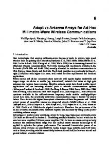
Linear array of 2N elements positioned along the x-axis.

209

In this paper, the use of the Particle Swarm Optimization technique to find the optimal radiation pattern of an adaptive antenna is proposed. By calculating the phase shift weights of a linear antenna array, the beam direction can be steered towards a desired angle. In addition, it is possible to place nulls at the direction of possible interferers. The present work compares these results with the ones obtained by using a Genetic Algorithm (GA) and shows that the PSO performs better in terms of power levels. Furthermore, for a desired array configuration, the number of fitness function evaluations performed by the PSO is shown to be less than the one from the GA. This can lead to an improvement in the overall performance of an adaptive array since its configuration must meet tough demands. First, in section II the geometry of a linear antenna array is explained and its array factor deduced. Then, in section III, an introduction to the Particle Swarm Optimization is presented. In section IV, the experiments and results of this work are discussed, and finally the conclusions are summarized in section V.

Figure 2.

and in its normalized form

II. L INEAR A NTENNA A RRAY

AFn (θ) =

Let us assume that the antenna under investigation is an array of 2N infinitesimal dipoles positioned along the x-axis equidistant from each other as shown in Figure 1. The total field of the array is equal to the field of a single element positioned at the origin multiplied by a factor which is widely referred to as the array factor. Thus, for the 2N element array, the array factor is given by [9] AF (θ) =

2N

wn e

Particle Swarm Optimization (PSO) is a biologicallyinspired optimization technique. It was first proposed by Eberhart and Kennedy in 1995 [1]. PSO is inspired by the social behaviour of bird flocking or fish schooling. In these biological systems, the collective behaviour of simple individuals in their environment leads to the solution of a given problem, for example, finding food. These individuals or particles fly the problem space which is associated with the best solution they have achieved so far. The system or swarm is initialized with a population of random solutions and searches for optima by updating generations (see Figure 2). Each particle remembers its best solution called personal best or pbest and the global best or gbest which is the best solution achieved so far by any of the individuals. At each iteration, the particles update their velocity towards the pbest and gbest locations according to the following equations

(1)

If the distance among elements is d and the reference point is the centre of the array, the array factor becomes αn ej[(n−N −0.5)ψ+βn ]

(2)

n=1

where 2N = number of antenna elements αn = amplitude weight at element n βn = phase shift weight at element n ψ = 2π λ d sin(θ) = kd sin(θ) θ = angle of interfering or desired signal

vn+1 = w ∗vn +c1 r1 (pbest,n −xn )+c2 r2 (gbest,n −xn ) (5)

In this work, only the phase shift weights are considered, so the amplitude weights are constant. And if the phase shifts are odd symmetry, the array factor can be written as AF (θ) = 2

(4)

III. PARTICLE S WARM O PTIMIZATION j(n−1)(kd cos(θ)+β)

ψ = kd cos(θ) + β

2N

N 1 cos[(n − 0.5)ψ + βn ] N n=1

This equation represents a mathematical description of the antenna radiation pattern and can be used by optimization algorithms. The PSO algorithm is able to search for optimal phase shift weights using a fitness function based on this array factor.

n=1

AF (θ) =

Particle Swarm Optimization flowchart.

N

cos[(n − 0.5)ψ + βn ]

xn+1 = xn + vn+1

(6)

where vn and xn are the particle velocity and position at the nth generation respectively. w is the inertia weight and

(3)

n=1

210

is used to control the trade-off between the global and the local exploration ability of the swarm, usually in the range of [0,1]. c1 and c2 are scaling constants that determine the relative pull of pbest and gbest , usually taken as c1 = c2 = 2.0. r1 and r2 are random numbers uniformly distributed in (0,1). Once the velocity has been calculated, the particle moves to its next location. The new coordinate is determined according to Equation 6. The swarm will continue moving until a criterion is met, usually a sufficiently good fitness or a maximum number of iterations.

The swarm size is set to 20 individuals. The inertia corresponds to the weight w and is fixed to 1.0. The correction factor are the constants c1 and c2 in the PSO velocity Equation 5. Previous work has shown that a value of 2.0 is a good choice for both parameters [11]. Initial positions are chosen at random inside the search space which is [−π; π] radians. This means that the algorithm must be configured to limit each particle position to those constrains. If a particle moves out of the the search space, its position is set to the previous value. The algorithm stops when the difference between successive fitness function values is less than the tolerance value, in this case, 1x10−6 . Given that there are two conditions to be met, the fitness consists of two functions: F (θ1 ) which will attempt to maximize the value of the array factor for the direction of user1 = -60◦ . While a second function, F (θ2 ) must minimize the array factor for the direction of user2 = 30◦ . The following fitness function is deduced

IV. R ESULTS The following example was used to demonstrate the performance of the PSO algorithm: Given a desired transmitter called user1 at the direction of -60◦ and an interferer transmitter called user2 at 30◦ , find a set of phase shifters that will configure a linear antenna array in such a way that the main lobe is directed to user1 whilst a null is presented to user2. For this problem, an array of 20 isotropic elements is defined, so N = 10 which is the dimension of the problem and the result consists of a vector x of 10 elements, each one corresponding to βn . Figure 3 shows an illustration of the desired radiation pattern.

F itness = F1 − F2

(7)

where F1

= =

2

|AF (θ1 )| 2 N 1 cos[(d − 0.5)k sin(θ1 ) + βn ] N n=1

(8)

and F2

= =

2

|AF (θ2 )| 2 N 1 cos[(d − 0.5)k sin(θ2 ) + βn ] N

(9)

n=1

Figure 3.

where θ1 and θ2 correspond to the angles of user1 and user2 respectively. A standard Genetic Algorithm (GA) is tested to compare its performance against the PSO. The Matlab function ga from the ”Genetic Algorithm and Direct Search Toolbox” is used. All parameters are left to their default values except for the population size which is set to 20, the maximum number of generations which is 500, the defined boundaries −π and π and the tolerance value that is the same as the PSO: 1x10−6 . Using the same tolerance for both algorithms ensures that they will attempt to reach a result within the same error of each other. After running the simulations, a vector of phase shift weights for each algorithm is obtained, xga and xpso as shown in Table II. The resulting radiation pattern in dβ (decibels) is shown in Figure 4. As can be seen, both algorithms successfully obtained a suitable set of phase shift weights that produce the desired radiation pattern. The main lobe is directed towards the angle of user1 = -60◦ , while a null in the direction of user2 = 30◦ is formed. It can also be noted that the PSO algorithm achieved a better radiation pattern than that obtained by the GA. The power of

Radiation pattern for desired and interfering angles -60◦ , 30◦ .

The geometry of the linear array is defined as follows: The distance d of any two adjacent elements is set to λ/2 = 2 where λ is the wavelength. k equals to (2π)/λ and represents the wavenumber. The PSO algorithm is programmed in Matlab and is based on the Standard PSO 2007 proposed by Maurice Clerc in [10]. The parameters are set as shown in Table I. Table I S ET OF PARAMETERS FOR THE PSO. Swarm size Inertia Correction factor Minimum boundary Maximum boundary Tolerance

20 1.0 2.0 −π π 1x10−6

211

the main lobe is higher for the PSO as well as the value of the null is lower. It was also observed that the PSO algorithm performed less number of fitness function evaluations than the GA. The PSO executed 1338 fitness function operations whereas the GA executed 1667.

Average number of fitness function evaluations against number of dimensions. 2400 GA PSO 2200

Average function evaluations (100 runs).

2000

Table II P HASE SHIFT VECTORS TO OBTAIN A MAIN LOBE AT -60◦ , NULL AT 30◦ . β β β β β β β β β β

xga = 1.4378 = -0.7943 = 1.0848 = 2.6372 = -0.2880 = 2.3845 = -0.1420 = 1.9148 = -0.8593 = 0.8625

β β β β β β β β β β

xpso = 1.2899 = -2.2126 = 0.5883 = 3.0162 = -0.3530 = 2.4889 = -1.2133 = 1.5080 = -1.9363 = 0.7529

1600

1400

1200

1000

800

600

5

10

Figure 5.

GA PSO −10

−15

−20

−25

−30

25

30

Average number of function evaluations against dimensions.

Table III P HASE SHIFT VECTORS FOR MAIN LOBE AT -60◦ , NULLS AT -20◦ , 40◦ .

−35

−40

Figure 4.

20

of the problem is N = 20. The rest of the parameters for both algorithms are the same as the first experiment. A set of 20 phase shift weights is obtained from the GA and PSO algorithms as shown in Table III. It is important to note that the fitness function must be modified for this problem since there is a third factor that affects its output. The new fitness function is given by Equation 10.

20−element array. Main lobe direction at −60º and nulling direction at 30º

−45 −100

15 Dimensions.

−5

Relative power pattern (dB)

1800

−80

−60

−40

−20

0 20 Theta (degrees)

40

60

80

β1 β2 β3 β4 β5 β6 β7 β8 β9 β10 β11 β12 β13 β14 β15 β16 β17 β18 β19 β20

100

Radiation pattern for desired and interfering angles -60◦ , 30◦ .

To further study this, the same experiment was run 100 times and the mean was calculated. Another factor to consider is the dimension of the problem or number of array elements. In Figure 5, the graph shows the total number of function evaluations executed by both algorithms over different dimensions. For a range of dimensions from 5 to 30, the GA performed more function evaluations than the PSO. This is important as a dynamic configuration of the array should meet the performance requirements according to the application. The total number of fitness function evaluations indicates the overall performance of the system, given that the fitness function evaluation is the most computationally intensive part of the algorithm. A second experiment was performed in which the capability of avoiding two different directions instead of one was tested. In this example, user2 is moved to the direction -20◦ , closer to the desired user1 which remains at -60◦ . A third undesired user, user3 appears in the direction 40◦ . The aim is to create nulls in user2 and user3 directions. This time, the number of antenna elements is set to 40 so the dimension

xga = 1.7244 = 0.6048 = 0.6785 = 2.3043 = 0.6309 = 1.9293 = 0.9169 = 1.2024 = 2.2653 = 0.9047 = 3.1094 = 0.9034 = 2.4115 = 0.3607 = 1.1969 = 0.3128 = 1.2371 = 2.8380 = 0.3142 = 2.8321

β1 β2 β3 β4 β5 β6 β7 β8 β9 β10 β11 β12 β13 β14 β15 β16 β17 β18 β19 β20

xpso = 1.5439 = -2.1608 = 0.4752 = 3.1413 = -0.2736 = -3.1392 = -1.2152 = 1.2778 = 3.1415 = 0.7004 = -2.9015 = -0.0983 = -3.1415 = -0.9601 = 1.4342 = -1.7718 = 0.9627 = -2.7192 = 0.0213 = 2.8388

F itness = F1 − F2 − F3

(10)

where F3 corresponds to the third condition which is a null at the direction of user3 = 40◦ . After simulating the GA and PSO algorithms, the resulting radiation pattern, shown in Figure 6, is obtained. Once more, it can be observed that both algorithms are able to optimize a set of phase shift weights that

212

40−element array. Main lobe direction at −60º and two nulling directions at −20º and 40º

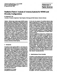
levels achieved by the GA are not as constant and oscillate between -5dβ and -10dβ. Similarly, the power radiated towards the undesired directions is generally lower in the case of the PSO compared with the ones obtained by the GA.

0 GA PSO −5


−10

−15

−20

V. C ONCLUSIONS

−25

In this paper, the Particle Swarm Optimization method was used to obtain a set of phase shift weights that configure a linear antenna array. These weights were optimized in order to maximize the power of the main lobe at a desired direction while keeping nulls towards interferers. A comparison with a Genetic Algorithm was studied and the results of 1000 experiments show that the PSO achieves better and more consistent radiation patterns than those of the GA. It was also observed that the total number of fitness function evaluations is lower for the PSO, which suggests an advantage in terms of performance as the function evaluation tends to have higher computational cost. At present, the possibility for optimizing both phase and amplitude is being investigated.

−30

−35

−40 −100

−80

−60

−40

−20

0 20 Theta (degrees)

40

60

80

100

Figure 6. Radiation pattern for desired angle -60◦ , and interfering angles -20◦ and 40◦ .

cause a main lobe and two nulls to point to the desired and interfering directions. Similar to the first experiment, the PSO algorithm performs generally better in terms of radiating power. Moreover, it can be noticed that the SideLobe Levels (SLL) which are the lobes other than the main lobe, are considerably lower for the PSO compared to those for the GA. This is often desirable as it helps to avoid other interfering signals at different directions other than the main lobe. These experiments suggest that the PSO algorithm tends to perform better than the GA algorithm in terms of higher power in the desired direction and lower power in the interfering directions. This leads to perform a third experiment to further study this: In order to observe if the PSO obtains in general better configurations, the second experiment with the same conditions was repeated 1000 times. The power at the main lobe and null directions (maximum and minimum levels) of user1, user2 and user3 for both algorithms was measured. The results of both PSO an GA algorithms are shown in Figure 7.

ACKNOWLEDGMENT The authors acknowledge the financial support from the Mexican National Council for Science and Technology (CONACyT), grant number 181512. R EFERENCES [1] J. Kennedy and R. C. Eberhart, “Particle swarm optimization,” in Proc. of the IEEE Int. Conf. on Neural Networks. Piscataway, NJ: IEEE Service Center, 1995, pp. 1942–1948. [2] R. C. Eberhart and Y. Shi, “Evolving artificial neural networks,” in Proc. 1998 Int. Conf. Neural Networks and Brain, Beijing, 1998. [3] J. Robinson, S. Sinton, and Y. Rahmat-Samii, “Particle swarm, genetic algorithm, and their hybrids: optimization of a profiled corrugated horn antenna,” in Proc. IEEE Int. Symp. Antennas Propagation, ser. vol. 1, San Antonio, TX, 2002, pp. 314–317.

Maximum and Minimum power pattern levels for the GA and PSO algorithms 0 GA PSO


−10

[4] C. Khodier, M.and Christodoulou, “Linear array geometry synthesis with minimum sidelobe level and null control using particle swarm optimization,” IEEE Transactions on Antennas and Propagation, vol. 8, no. 53, pp. 2674–2679, August 2005.

−20

−30

−40

[5] J. Robinson and Y. Rahmat-Samii, “Particle swarm optimization in electromagnetics,” IEEE Transactions on Antennas and Propagation, vol. 2, no. 52, pp. 397–407, February 2004.

−50

−60

0

Figure 7. algorithms.

100

200

300

400 500 600 Number of experiments

700

800

900

1000

[6] J. Kennedy and W. M. Spears, “Matching algorithms to problems: an experimental test of the particle swarm and some genetic algorithms on multi modal problem generator,” in Proc. IEEE Int. Conf. Evolutionary Computation, 1998.

Main lobe and nulls power values for the GA and PSO

[7] M. Shihab, Y. Najjar, N. Dib, and M. Khodier, “Design of non-uniform circular antenna arrays using particle swarm optimization,” Journal of electrical engineering, vol. 59, no. 4, pp. 216–220, 2008.

It can be observed that the power of the main lobe obtained by the PSO algorithm is generally maintained around -5dβ for almost all of the 1000 experiments while the

213

[8] C.-H. Hsu, W.-J. Shyr, and C.-H. Chen, “Adaptive pattern nulling design of linear array antenna by phase-only perturbations using memetic algorithms,” Innovative Computing, Information and Control, 2006. ICICIC, vol. 3, pp. 308–311, Aug 2006. [9] C. A. Balanis, Antenna Theory: Analysis and Design, 3rd ed. Arizona State University, 2005. [10] M. Clerc, http://clerc.maurice.free.fr/pso/, [Accessed: March 2010]. [11] R. C. Eberhart and Y. Shi, “Particle swarm optimization: Developments, aplications and resources,” in Proc. 2001 Congr. Evolutionary Computation, ser. vol. 1, 2001.

214