Gaussian noise; finally, our search strategy is multi-scale, for fast convergence, and ..... V.R. Mandava, J.M. Fitzpatrick and D.R. Pickens, III,. "Adaptive Search ...
ITERATIVE MULTI-SCALE REGISTRATION WITHOUT LANDMARKS Philippe Thévenaz, Urs E. Ruttimann and Michael Unser National Institutes of Health Bethesda MD 20892–5766, USA
ABSTRACT We present an automatic sub-pixel registration algorithm that minimizes the mean square difference of intensities between a reference and a test data set (volumes or images). It uses spline processing, is based on a coarse-to-fine pyramid strategy, and performs minimization according to a variation of the iterative Marquardt-Levenberg scheme. The geometric deformation model is a general affine transformation that one may optionally restrict to a rigid-body (isometric scale, rotation and translation), procrustean (rotation and translation) or translational case; it also includes an optional parameter for the linear adaptation of intensity. We present several PET and fMRI experiments and show that this algorithm provides excellent results. We conclude that the multi-resolution refinement strategy is faster and more robust than a comparable single-scale one.
1. INTRODUCTION Image registration plays a major role in at least two types of application: data fusion, where noise reduction is often desired, and data comparison, for the detection of significant differences. In the first case, one takes advantage of the availability of multiple instances of supposedly identical data. The registration of these instances with one another allows the extraction of common features, for example by averaging, or by more refined processes [1]. One can find successful examples of this approach in the correlation-averaging of virus particles in high-resolution electron microscopy [2]. It has also been applied in the consolidation of sparse data, for example when mapping range images of the sea floor [3]. In the second case, a new problem appears, due to the very fact that the registration process tries to align data that are possibly dissimilar. This last consideration sometimes leads to robust registration methods using an internal criterion that is not sensitive to outliers [4, 5, 6]. After registration, the task usually proceeds by the detection of dissimilar regions, given a statistically significant level of confidence in the decision with respect to the type I and type II errors [7]. Be it fully automated [8] or not [9], landmark registration is often proposed as a versatile solution. It allows for a geometric transformation whose properties can be as general as desired [10], or in the contrary be tuned to the problem by additional constraints [11, 12]. However, the solution can be no better than the initial selection of landmarks allows, which is the crucial component of this approach; moreover, it fails when sub-pixel accuracy is desired, since the landmarks are usually selected directly on the discretization grid. Registration without landmark is the preferred solution whenever applicable, since it often takes into account the whole of the available data by implementing some kind of correlation process. The resulting benefit is that the robustness of this class of techniques is much higher than that of landmark-based registration [4]. One may consider any kind of geometric transformation, be it local and computationally expensive, like a deformation field [13], or inexpensive, but restricted to a global translation [14]. In this paper, we address the problem of registration for data comparison purposes, without landmarks, and with a global affine transformation paradigm. This transformation is more general than the one used in [15]. We present a fully automatic iterative multi-scale registration with sub-pixel accuracy, extending the work in [16] by considering a full tri-dimensional (3-D) approach. In the terminology of [17], we use the raw intensity as our feature space, thus effectively exploiting all the information in the image; our search space is the
continuous set of non-singular 3-D affine transforms, which are the most general linear transformations available, and where by continuity we imply sub-pixel accuracy; our dissimilarity measure is Euclidean, which is maximum-likelihood assuming additive white Gaussian noise; finally, our search strategy is multi-scale, for fast convergence, and iterative, based on a variation of the MarquardtLevenberg (ML) algorithm for non-linear least-square optimizations [18].
2. SYSTEM 2.1. Criterion Any automatic registration method requires the optimization of an objective criterion, whose role is to measure the similarity of the test data with respect to the reference. As criterion, we select ε 2 the average square difference. Letting f R (x ) and f T (x) be respectively the reference and test data, our criterion reads ε2=
1 V
∫x∈V ( f R (x) −Qp { f T( x)} ) d x 2
(1)
where Qp { f } is the transformation of interest described by p , and where V represents the volume of interest. This criterion offers the advantage that it is well understood and lends itself well to minimization with respect to p . Its drawback is that, in the presence of severe outliers, its minimum may become less pronounced, and may not even be located where one would expect it to be. In our case (medical imaging), outliers do exist, for example when we compare two functional magnetic resonance images (fMRI) of a brain in two different states of activation. However, we do not expect these outliers to be dominant; in fact, the very need for registration arises from the fact that the differences between the two brain instances are extremely faint, and cannot be detected without their careful alignment. 2.2. Transformation As transformation of interest Qp {ƒ } , we consider the general affine transformation described by a 3 × 3 matrix A and by a translation vector b Qp {ƒ (x)} = QA ,b { ƒ( x) } = ƒ (A x + b)
(2)
This transformation includes translation, rotation around any center, skewing, shearing and scaling. We have also developed more constrained versions (e.g., rigid body, procrustean, translation only), and, as in [4], we have added to all of them a possibility for gray-scale adaptation; but we do not report on any of these extra versions here. 2.3. Multi-scale processing We will see below that our approach is iterative. We presently take advantage of this fact by introducing a change of resolution between some of the iterations. Using a coarse-to-fine strategy enables us to perform a first parameter estimation at the coarsest level of a resolution pyramid; after this first estimation is deemed satisfactory, we switch to a finer level, using the previous parameters as initial conditions for carrying the optimization on the new level. At each new level the convergence is fast, since these propagated initial conditions are close to the actual optimum. In fact, for practical purposes, the quasi-Newtonian optimization method that we use can converge in just one step if the previous estimate is sufficiently good, which is often the case for all but the coarsest level where most of the iterations are spent, but where fortunately
the data set is small. This saving reflects itself in the computation time, which is greatly reduced. Another very important advantage of using a resolution pyramid is that its embedded smoothing properties tend to regularize the problem by letting the surface ε 2(p) be also smoother at coarser scales: the image size reduction effectively removes most of the noise. With most images, it is very likely that the location of a near-absolute optimum in the coarsest level will not be missed, whereas it would possibly be, if only the finest level would be looked at. This is important since, contrary to [19], we do not make use of an optimization procedure that would be able to escape from local minima. The pyramid is computing according to [20, 21] with cubic splines. Initial parameters
{
New parameters
Delay
Geometric transformation
Comparison
AA {Tb{ ƒ (x) }} =ƒ (A(x +b )) = TAb { AA { ƒ( x)}}
These operators are distributive with respect to the addition Tb {ƒ (x) + g( x)} = Tb {ƒ(x)} +T b {g(x )} AA {ƒ (x) + g( x)} = AA {ƒ (x)} + AA {g (x) } Looking at the squared norm of the signal, we have 2
= ƒ ( x)
{
Disparity minimization
2.4. Optimization Our choice for solving ∂ε 2 (p) ∂p = 0 is ML, an iterative gradientbased algorithm for non-linear least-squares optimization problems [18]. The system is depicted in Figure 1, where we see that at each step f T (x) has to undergo Qp {ƒ } before it is compared to f R (x ). The reslicing needed in the geometric transformation is performed by resampling a cubic spline model fitted to the volume. The optimization requires the explicit knowledge of the partial derivatives ∂ f T ∂ p , which are computed by using a cubic spline fit again, along with the techniques described in [20, 21]. In section 3 we will propose an approach to further accelerate the standard ML algorithm when the transformation satisfies certain commutativity and distributivity rules. 2.5. Convergence We consider three concurrent criteria for deciding when to stop the iteration process. The first one is self-evident: we stop when a nearperfect match is met, that is, when ε 2 ≤ T , where T is some prescribed threshold. The second has to do with the observed relative gain ∆ε2 ε2 at each successful iteration step: we declare that the convergence is reached whenever this gain is below another user-selected threshold. The third one concerns itself with ∆pi pi the relative change of parameter values at every iteration step: when at least one of the parameters is alive, we keep on going; but when all are motionless we stop. If any parameter pi happens to be zero, or near zero, we substitute ∆pi pi by a similar, although possibly less effective criterion extracted from some of the parameters of the ML algorithm, guaranteed not to suffer from normalization problems, and guaranteed to converge towards zero when the number of iterations grows high enough.
3. ACCELERATED MARQUARDT-LEVENBERG 3.1. Requirements Let us decompose the operator Qp {ƒ } into a translation and a matrix operation given respectively by The composition rules for these operators are
(5)
AA{ ƒ (x) } = ƒ (x) 2
2
}
{
}
ε 2 = AI+ ∆A T ∆b {f T (x )} − AA−1 T −b { f R (x) }
Figure 1: Outline of the registration algorithm
AA {ƒ ( x)} = ƒ (A x)
(4)
2
A
(6)
3.2. Criterion revisited Using the previous expressions, we can now rewrite a criterion exactly equivalent to (1) as
Incremental update
Reference volume
Qb {ƒ (x)} = ƒ( x + b)
}
Tb { AA{ ƒ(x)}} =ƒ (Ax +b) = AA TA −1b { ƒ( x)}
Tb {ƒ (x)}
Actual parameters Test volume
Tb {T a { ƒ(x)}} =ƒ (x + a + b) = T a+b {ƒ (x) }
AB{ AA{ ƒ (x) }} = ƒ (B A x) = ABA {ƒ(x )}
(3)
2
(7)
{
}
ε2=
⋅ f T (x ) − A I+∆ A −1 A−1 T −b− A( I+∆A ) ∆b { f R (x) } ( ) I+∆A
ε2=
A ⋅ T b+A( I+∆A )∆b AA (I+ ∆A) { f T(x)} − f R (x)
1
{
}
2
(8)
2
(9)
Minimizing (7) with respect to ∆p =( ∆A ,∆b) is equivalent to the more traditional minimization of (9) with respect to p when written with ∆p = 0 . The advantage of the minimization over ∆p instead of p is that the Hessian matrix required in ML has now to be computed once only, at the parameter value ∆p = 0 ; the same is true for the derivatives (∂ f T ∂ ∆p) . ∆p= 0 It also simplifies the dependencies between the ∆pi parameters, the only cost being a slightly more complicated parameter update procedure, that is, p → p + ∆p has to be replaced by the set of rules given in (8). In essence, we now update the transformation that is applied to f R instead of f T . 3.3. Level change Since our approach is pyramidal, at each level change we not only have to compute new derivatives and Hessian, but we also need to update the parameters between levels. Consider an initial geometric transformation Tb { AA {ƒ(x)}} given by y1 = b1 +a11x 1 + a12 x2 +a13 x 3 y 2 = b2 + a 21x1 + a22 x 2 + a23x3 y3 = b3 + a31 x1 + a32 x2 + a33 x 3
(10)
Apply some scale factors ( λ 1,λ 2 ,λ 3 ) and compute a new, equivalent transformation Tb ′ { AA ′{ s( x ′)}} as in ′ x1′ + a12 ′ x′2 + a13 ′ x′3 y1′ = b1′ + a11 ′ x1′ + a22 ′ x2′ + a′23x3′ y2′ = b′2 + a 21 ′ x1′ + a32 ′ x2′ + a33 ′ x′3 y3′ = b′3 + a31
x1′ = λ 1x 1 x2′ = λ 2x 2 x3′ = λ 3x 3
y1′ = λ 1y 1 y2′ = λ 2 y2 y′3 = λ 3 y3
(11)
These four systems of three equations are satisfied by λ λ a′ = a a12 ′ = λ 1 a12 a13 ′ = λ 1 a13 2 3 b1′ = λ1 a1 11 11 λ λ ′ = λ 2 a21 a22 ′ = a22 a 23 ′ = λ2 a23 b2′ = λ 2a1 a21 1 3 b3′ = λ 3 a1 a′ = λ 3 a a′ = λ 3 a a′ = a 33 31 λ 1 31 32 λ 2 32 33
(12)
This last equation allows us to carry a description of the geometric transformation from one level of the pyramid to the next. It also needs to be applied at the change of level, when the origin of the coordinate system is displaced.
4. EXPERIMENTS 4.1. Ideal case We begin our experiment series with a noise-free case, and we further simplify the problem by considering an image instead of a volume. First, we scale by λ , rotate by θ = 5° and translate by (dx,dy) = (5,5) the Lena image using cubic spline resampling. We then use this image as our reference and try to align the original towards it. Since our registration procedure also uses cubic spline resampling, an exact match is a priori not impossible. Table 1 gives the considered parameters (including N the number of levels in the pyramid and t the relative computation time), their estimation by our registration algorithm, and the residual error ε 2 expressed in dB as a SNR between the aligned f T (x) and f R (x ). i ii N 4 4 t 0.30 0.23 d x′ 5.0010 5.0002 d y′ 5.0057 5.0002 θ ′ 5.0070 5.0003 λ ′ 0.7999 1.2500 λ 0.8 1.25 ε 2 42.05 43.29
iii iv 4 3 0.22 0.22 4.9983 4.9983 5.0018 5.0018 5.0015 5.0015 1.0000 1.0000 1 1 43.26 43.26
v vi 2 1 0.31 1.00 4.9984 4.9999 5.0016 4.9992 5.0014 5.0035 1.0000 0.9999 1 1 43.28 43.03
Table 1: Ideal registration experiment In this table, θ′ has been estimated from the general affine transformation, and λ ′ from its determinant ( λ is the correct value). We see that the fit is almost perfect, the relative error on the parameter estimation being most of the time lower than 1‰ . We even had to resort giving many digit figures for showing the accuracy of the estimates. 4.2. Noisy case We now add some white Gaussian noise to the previous test and reference images and we observe its effect on the registration. The amount of added noise is the same for f T (x) and f R (x ), is independent for each of both images, and is reported in dB. Table 2 shows the results of these experiments, with N = 4 , (dx,dy) = (5,5) , θ = 5° , and λ =1. i ii SNR 25 20 d x′ 4.9981 5.0008 dy ′ 5.0022 4.9988 θ′ 5.0005 5.0024 λ′ 0.9999 1.0000 ε2 23.86 18.46
iii iv 15 10 4.9918 4.9883 5.0170 5.0314 5.0027 5.0112 0.9999 1.0000 13.34 8.35
v 5 4.9629 5.0533 5.0447 0.9997 4.05
∆x ∆x ′ θ θ′
i 0.800 0.820 0.23 0.23
ii 1.333 1.372 0.47 0.47
iii 2.133 2.186 0.70 0.66
iv 2.667 2.735 0.93 0.87
v vi 2.933 3.003 1.17 1.40 1.09 1.37
Table 3: Two fMRI experiments We see that the agreement between the synthetic and the estimated displacements is fairly good; the same can be said of the measured and the estimated angle of rotation. Unfortunately, the precision of the mechanical device used for rotating the phantom is unknown; but the true difference θ − θ′ can be considered to lie within a tenth of a degree. We should add here that the limited range we explored was constrained by mechanical limitations. Given the identity transformation as initial guess, other experiments have shown that our registration algorithm still converges for angles as big as 30˚ . 4.4. Uncontrolled 3-D PET brain scans In the previous experiments we showed cases where the deformation model (affine transformation) was consistent with the data. In the next example, this assumption will be no more valid: consider brain volumes acquired through a Positron Emission Tomography (PET) imaging device, and take several patients into account. The goal is now to register these brains with one another. Since they belong to different subjects, they exhibit not only size differences but also shape differences, which introduces outliers in the statistics of the difference volume. Figure 2 shows a set of unregistered slices of several patients, cut at the same nominal position in the original volumes. The top left is the reference slice, and the bottom right is the average of the selected slice for all 32 patients. Figure 3 shows the same configuration after registration in 3-D.
vi 0 4.9058 5.1996 5.1102 0.9995 0.77
Table 2: Noisy registration experiment Even when the signal is in a one-to-one ratio with noise (0 dB case), the parameter estimation is still very good (the relative error is lower than 5% ). In this experiment, like in the previous one, we used the identity transformation as initial condition for the registration algorithm. 4.3. Controlled 3-D fMRI phantom For this experiment, we used a 3-D phantom acquired through the functional Magnetic Resonance Imaging (fMRI) system described in [22]. We performed two separate sets of experiments. In the first one, we reconstructed the phantom from the Fourier domain with an added linear phase (synthetic translation); in the second one, we physically rotated the phantom by a known angle. Tables 3 shows the respective results of these two experiments, where ∆x (in voxel units) stands for the synthetic displacement, ∆x ′ for its estimation through our registration procedure, and where θ (in degrees) stands for the measured physical rotation and θ′ for its estimation.
Figure 2: Unregistered slices and their average
Figure 3: Registered slices and their average
In our registration algorithm, the specification of V , from equation (1), allows one to mask out irrelevant features. Since PET images are typically noisy, we took advantage of this masking and ignored most of the background contribution, which explains the disappearance of streaks in Figure 3. Regarding the success of the registration, it is clear that most of the brain features are better resolved in the registered average volume than in the unregistered one (lower-right part of Figures 4 and 3 respectively). It tends to show that our least-squares registration criterion is robust enough to cope with outliers, i.e., deformations that cannot be modeled by an affine transformation. Another kind of outliers, not striking in the displayed figures but nevertheless present, has to do with the fact that the intensity contrast of the volumes differs from one patient to the next. Our registration algorithm can take this effect into account and determine a best linear remapping of the intensity that, when applied concurrently with the geometric affine transformation, minimizes the criterion shown in equation (1).
5. CONCLUSION We have described a fully automatic registration algorithm that uses raw intensity as feature space and considers a Euclidean least-squares criterion for the simultaneous determination of a general 3-D affine transformation and of a linear change of intensity contrast. The search strategy takes advantage of a resolution pyramid and is based on a variation of the Marquardt-Levenberg algorithm for non-linear leastsquares optimization. We perform all the processing steps with cubic spline models. We have implemented this algorithm and we have presented several experiments involving 2-D images and 3-D volumes as well. We were able to show a good performance of our algorithm through a whole range of cases (synthetic problem, synthetic problem with added noise, controlled 3-D experiment with real data, real data with geometric outliers and intensity outliers). An attractive feature of this registration algorithm is that it can easily incorporate a priori knowledge by the way of a (possibly multi-valued) mask. Another attractive feature is that the user can constrain the general affine transformation to be a rigid-body transformation, or even a procrustean transformation. Finally, the cost, in terms of computation time, is minimized through the use of a resolution pyramid.
REFERENCES [1]
[2]
[3]
[4]
[5]
[6]
M. Irani and S. Peleg, "Improving Resolution by Image Registration," Computer Vision, Graphics, and Image Processing, vol. 53, no. 3, pp. 231–239, 1991. J. Frank, A. Verschoor and M. Boubik, "Computer Averaging of Electron Micrographs of 40S Ribosomal Subunits," Science, vol. 214, pp. 1353–1355, 1981. B. Kamgar-Parsi, J.L. Jones and A. Rosenfeld, "Registration of Multiple Overlapping Range Images: Scenes without Distinctive Features," IEEE Trans. Pattern Analysis and Machine Intelligence, vol. 13, no. 9, pp. 857– 871, 1991. M. Herbin, A. Venot, J.-Y. Devaux, E. Walter, J.-F. Lebruchec, L. Dubertret and J.-C. Roucayrol, "Automated Registration of Dissimilar Images: Application to Medical Imagery," Computer Vision, Graphics, and Image Processing, vol. 47, no. 1, pp. 77–88, 1989. J.Y. Chiang and B.J. Sullivan, "Coincident Bit Counting— A New Criterion for Image Registration," IEEE Trans. Medical Imaging, vol. 12, no. 1, pp. 30–38, 1993. A. Venot, L. Pronzato and E. Walter, "Comments about the Coincident Bit Counting (CBC) Criterion for Image Registration," IEEE Trans. Medical Imaging, vol. 13, no. 3, pp. 565–566, 1994.
[7]
[8]
[9]
[10] [11]
[12]
[13]
[14]
[15]
[16]
[17]
[18]
[19]
[20]
[21]
[22]
U.E. Ruttimann, M. Unser and D. Rio, "Statistical Analysis of Image Differences by Wavelet Decompositions," in Proc. 16th Annual Int. Conf. of the IEEE Engineering in Medicine and Biology Society, Baltimore, Maryland, U.S.A., November 3-6, 1994, pp. 28a–29a. Q. Zheng and R. Chellappa, "Motion Detection in Image Sequences Acquired from a Moving Platform," in Proc. Int. Conf. Acoustics, Speech, and Signal Processing, Minneapolis, Minnesota, U.S.A., April 27-30, 1993, pp. V-201–V-204. G.Q. Maguire, Jr., M.E. Noz, H. Rusinek, J. Jaeger, E.L. Kramer, J.J. Sanger and G. Smith, "Graphics Applied to Medical Image Registration," IEEE Computer Graphics and Applications, pp. 20–28, 1991. J. Flusser, "An Adaptative Method for Image Registration," Pattern Recognition, vol. 25, no. 1, pp. 45–54, 1992. B.C.S. Tom, S.N. Efstratiadis and A.K. Katsaggelos, "Motion Estimation of Skeletonized Angiographic Images Using Elastic Registration," IEEE Trans. Medical Imaging , vol. 13, no. 3, pp. 450–460, 1994. T. Wakahara, "An Iterative Image Registration Technique Using Local Affine Transformation," Systems and Computers in Japan, vol. 21, no. 12, pp. 78–89, 1990. Y. Amit, "A Nonlinear Variational Problem for Image Matching," SIAM Journal on Scientific Computing, vol. 15, no. 1, pp. 207–224, 1994. J. Noack and D. Sutton, "An Algorithm for the Fast Registration of Image Sequences Obtained with a Scanning Laser Ophtalmoscope," Physics in Medicine & Biology, vol. 39, no. 5, pp. 907–915, 1994. R.P. Woods, S.R. Cherry and J.C. Mazziotta, "Rapid Automated Algorithm for Aligning and Reslicing PET Images," Journal of Computer Assisted Tomography, vol. 16, no. 4, pp. 620–633, 1992. M. Unser and A. Aldroubi, "A Multiresolution Image Registration Procedure Using Spline Pyramids," in Proc. SPIE, San Diego, California, U.S.A., July 15-16, 1993, pp. 160–170. L.G. Brown, "A Survey of Image Registration Techniques," ACM Computing Surveys, vol. 24, no. 4, pp. 325–376, 1992. D.W. Marquardt, "An Algorithm for Least-Squares Estimation of Nonlinear Parameters," Journal of the Society for Industrial and Applied Mathematics, vol. 11, no. 2, pp. 431–441, 1963. V.R. Mandava, J.M. Fitzpatrick and D.R. Pickens, III, "Adaptive Search Space Scaling in Digital Image Registration," IEEE Trans. Medical Imaging, vol. 8, no. 3, pp. 251–262, 1989. M. Unser, A. Aldroubi and M. Eden, "B-Spline Signal Processing: Part I—Theory," IEEE Trans. Signal Processing, vol. 41, no. 2, pp. 821–832, 1993. M. Unser, A. Aldroubi and M. Eden, "B-Spline Signal Processing: Part II—Efficient Design and Applications," IEEE Trans. Signal Processing, vol. 41, no. 2, pp. 834–848, 1993. P. van Gelderen, N.F. Ramsey, G. Liu, J.H. Duyn, J.A. Frank, D.R. Weinberger and C.T.W. Moonen, "Three Dimensional Functional MRI of Human Brain on a Clinical 1.5T Scanner," Proceedings of the National Academy of Sciences, vol. in Press, 1995.