Jun 7, 2016 - SPEECH SOURCE SEPARATION IN REAL ROOM ENVIRONMENTS. Waqas Rafique ... the proposed multivariate Student's t source prior can consis- tently achieve ... the separation performance has become a research focus. Even though the .... proper evaluation of a BSS algorithm for real environments.
IVA ALGORITHMS USING A MULTIVARIATE STUDENT’S T SOURCE PRIOR FOR SPEECH SOURCE SEPARATION IN REAL ROOM ENVIRONMENTS Waqas Rafique, Syed Mohsen Naqvi, Philip J.B. Jackson, Jonathon A. Chambers Center for Vision, Speech and Signal Processing, Department of Electronic Engineering, University of Surrey, GU2 7XH, UK {w.rafique, s.m.r.naqvi, p.jackson, j.a.chambers}@surrey.ac.uk ABSTRACT
order dependencies across frequencies and defines each vector source prior by a dependent multivariate super Gaussian distribution, instead of independent univariate distributions used by traditional FD-CBSS approaches such as the ICA method. Such modelling imposes inter-vector source independence whilst preserving the higher order intra-vector source dependencies, namely the structural dependency between the frequency components of each source. Therefore, the IVA algorithm mitigates the permutation problem in the learning process and no prior or post processing is required. Recently, selecting the appropriate multivariate source prior to improve the separation performance has become a research focus. Even though the IVA algorithm mitigates the permutation problem, its separation performance and convergence speed still needs improvement in order to apply it in real room environments. Therefore to achieve faster convergence the fast fixed point IVA (FastIVA) method was proposed which applies Newton’s Method in the learning algorithm [9]. In this paper, we adopt a multivariate Student’s t distribution as a source prior for the IVA algorithm. This source prior has heavier tails which can be useful in modelling high amplitude components in speech signals, such as in voiced sounds. Thus such a source prior is likely to yield improved separation performance as compared with the original multivariate super Gaussian distribution employed in IVA, when used as the vector source prior. Moreover, the multivariate Student’s t source prior can also be used for the FastIVA to improve convergence rate. Furthermore, both the IVA and the FastIVA algorithms using the proposed Student’s t source prior are tested with real room impulse responses, instead of previously used synthetic room impulse responses [19]. The experimental results show that, with application of the proposed source prior, consistently improved and faster separation performance can be achieved in realistic scenarios. The remainder of the paper is organised as follows: Section 2 describes the IVA and the FastIVA algorithms; the IVA and the FastIVA with the proposed Student’s t source prior are explained in Section 3; results are shown in Section 4; finally conclusions and relations to prior work are discussed in Section 5.
The independent vector analysis (IVA) algorithm employs a multivariate source prior to retain the dependency between different frequency bins of each source and thereby avoids the permutation problem that is inherent to blind source separation (BSS). In this paper, a multivariate Student’s t distribution is adopted as the source prior, which because of its heavy tail nature can better model the large amplitude information in the frequency bins. Therefore it can improve the separation performance and the convergence speed of the IVA and fast version of the IVA (FastIVA) algorithms as compared with the IVA algorithm based on another multivariate super Gaussian source prior. Separation performance with real binaural room impulse responses (BRIRs) is evaluated by detailed simulation studies when using the different source priors, and the experimental results confirm that the IVA and the FastIVA with the proposed multivariate Student’s t source prior can consistently achieve improved and faster separation performance. Index Terms— Fast fixed point independent vector analysis, multivariate Student’s t distribution, binaural room impulse responses, source separation 1. INTRODUCTION Independent component analysis (ICA) is the central tool for the blind source separation (BSS) problem [1]. The most well-known BSS problem is the cocktail party problem, in which the desired speaker must be separated from a mixture of sounds [2, 3]. In the real room environment, due to reverberations, it becomes convolutive blind source separation (CBSS) [4]. Time domain methods for CBSS are computationally complex [5]. To overcome this problem the frequency domain (FD) approach was introduced [6]. Although this method reduces the computational cost, it introduces a significant permutation problem across the frequency bins, that is inherent to the BSS problem and various methods have been suggested for its resolution [7]. Independent vector analysis (IVA) on the other hand is proposed as an algorithmic approach to solve the permutation problem in FD-CBSS [8]. This IVA method exploits higher
978-1-4673-6997-8/15/$31.00 ©2015 IEEE
474
ICASSP 2015
2. INDEPENDENT VECTOR ANALYSIS
quadratically and it is free from selecting an efficient learning rate. The objective function for FastIVA is as follows [10]:
The noise-free model in FD-CBSS is described as x(k) = H(k)s(k) ˆs(k) = W(k)s(k)
J=
(1)
i=1
(2)
= const −
log|det(W (k))| −
n X
h
0
K X
|ˆ si (k 0 )|2 )x(k)
i
k0 =1
(7) where G0 (·) and G00 (·) denote the first derivative and second derivative of G(·) respectively and (·)∗ is the complex conjugate. If this is used for all sources, an unmixing matrix W(k) can be constructed which must be decorrelated with
(3) E[logq(ˆsi )]
W(k) ← (W(k)(W(k))† )−1/2 W(k).
(8)
By carefully selecting the appropriate source prior for the FastIVA algorithm, the separation performance and the convergence speed can be improved. 3. IVA WITH STUDENT’S T SOURCE PRIOR The nonlinear score function is used to preserve the interfrequency dependency and to improve the performance of the IVA algorithm. A new statistical model that can better preserve the dependency within the source vector is still needed. It is also stated in [8] that the non-linear function is derived based on the PDF of the source, so performance of the algorithm can be improved by selecting a source prior that is more appropriate for speech signals. Therefore in this paper we have considered the multivariate Student’s t source prior, which because of its heavy tails can generally better model the spectrum of speech signals [16].
where (.)† denotes the Hermitian transpose and µi and Σ−1 i are the mean vector and inverse covariance matrix of the i-th source respectively. When the cost function (3) is minimised by the gradient descent method, the nonlinear score function for source ˆsi can be obtained as [8]: ∂logq(ˆ si (1) · · · sˆi (k)) ∂ˆ si (k)
k=1
− E (ˆ si (k))∗ G (
where E[·] denotes the statistical expectation operator, and det(·) is the matrix determinant operator. In the above equation, each source is a multivariate vector and the cost function would be minimised when the vector-sources are independent while the dependency between the components of each vector is still preserved. The inter-frequency dependency is modelled by the PDF of the source. The original IVA algorithm exploits a particular multivariate super Gaussian distribution as the source prior, which can be written as: � � q −1 † (4) q(si ) ∝ exp − (si − µi ) Σi (si − µi )
ϕ(k)(ˆ si (1) · · · sˆi (k)) = −
k=1
k0 =1
i=1
k=1
k=1
(6) where wi (k)† and λi (k) are the i-th row of the unmixing matrix W(k), and the i-th Lagrange multiplier respectively. G(.) is the nonlinear function of the summation of the desired signals in all frequency bins. The nonlinear function is derived from the source prior which can take on several different forms as discussed in [9]. For FastIVA with normalisation, the learning rule is: K K i h 0 X 00 X wi (k) ←E G ( |ˆ si (k)|2 ) + |ˆ si (k)|2 G ( |ˆ si (k)|2 ) wi (k)
where x(k) = [x1 (k), x2 (k) · · · xm (k)]T is the observed signal vector, and ˆs(k) = [ˆ s1 (k), sˆ2 (k) · · · sˆn (k)]T is the estimated signal vector both in the frequency domain and (.)T denotes vector transpose. The index k denotes the k-th frequency bin of this multivariate model. H(k) and W(k) are the mixing matrix and the unmixing matrix respectively. In this paper we assume that the number of sources m is the same as the number of microphones n, i.e. m = n The Kullback-Leibler divergence between the joint probability density function p(ˆs1 · · · ˆsn ) and the product of probability Q density functions (PDFs) of the individual source vectors q(ˆsi ) is used to derive IVA [8]. � � Y J = KL p(ˆs1 · · · ˆsn )|| q(ˆsi ) K X
n h K K i X � X � X E G( |ˆ si (k)|2 ) − λi (k){wi (k)† wi (k) − 1}
(5)
3.1. Multivariate Student’s t distribution The Student’s t distribution is now defined. A K-dimensional random source vector s = (s1 , . . . , sK )T is said to have a K-variate t distribution with degree of freedom ν, mean µ and covariance matrix Σ, if its joint PDF is given by [17]:
where ϕ(k)(ˆ si (1) · · · sˆi (k)) is a multivariate score function and is used to retain dependency across the frequency bins and k is the number of frequency bins. 2.1. IVA with the Newton Method The fast fixed point IVA algorithm is a rapidly converging form of the IVA algorithm that uses second order learning i.e. Newton’s method in the update. Newton’s method converges
f (s) = √
475
ν+K � Γ( ν+K (s − µ)T Σ−1 (s − µ) �− 2 2 ) 1 + ν νπΓ( ν2 )|Σ|1/2 (9)
The degree of freedom parameter ν can tune the variance and leptokurtic nature of the distribution. With decreasing ν, the tails of the super Gaussian distribution become heavier. Recently, the multivariate Student’s t distribution has been used to model speech signals [15]. The Student’s t distribution is a super Gaussian distribution, which has heavier tails than the Gaussian distribution and thus it is more suitable to model certain types of speech signals [16]. Due to the nature of speech signals, many useful samples can be of high amplitude. Thus the long tails can be an advantage when modelling the dependency between different frequency bins of a speech signal. This advantage of the Student’s t distribution will be exploited in the IVA algorithm by changing the source prior from a multivariate Gaussian distribution to a multivariate Student’s t distribution. The proposed multivariate student’s t distribution as the source prior takes the form �− ν+K � 2 (si − µi )† Σ−1 i (si − µi ) (10) q(si ) ∝ 1 + ν
proper evaluation of a BSS algorithm for real environments. In this paper, we have performed new evaluations using real binaural room impulse responses (BRIRs). The BRIRs that were recorded by Shinn-Cunningham, in a real classroom were used for the simulations [20]. Six different source location azimuths (15 ◦ − 90 ◦ ) relative to the second source were used. Also, for reliability all measurements were repeated on three separate occasions. The measurements shown are the average of three measurements at six different angles to obtain a better average estimate of the separation performance. The RT60 of 565ms examines the achieved performance of the algorithm in a difficult and highly reverberant real room environment.The signal-to-distortion ratio (SDR) in decibels (dB) calculated with the SiSec toolbox [21] is used to evaluate the separation performance. In all the experiments, we used the TIMIT dataset [23]. In each experiment we chose two different speech signals randomly from the TIMIT dataset and convolved them into two mixtures. We found empirically that ν = 4 was an appropriate value for the degrees of freedom parameter in the Student’s t source prior and the same value was used for all the experiments in this paper. The common parameters used in all experiments are given in Table 1.
We assume a zero mean vector µi and that Σi is an identity matrix. As such, with appropriate normalisation the nonlinear function can be used for both the gradient descent IVA and the FastIVA in the following ways.
Table 1: DIFFERENT PARAMETERS USED IN EXPERIMENTS.
• For the gradient descent IVA, the non linear score function can be derived as shown in our previous work [11]: ϕ(k)(ˆ si (1) · · · sˆi (k)) ∝
ν+K ν 1+
1 ν
STFT frame length Velocity of sound Reverberation time Room dimensions Source signal duration
sˆi (k) PK
|ˆ si (k)|2 (11) can be absorbed by the step size in The coefficient ν+K v the update equation. Thus it can be normalised to unity. k=1
1024 343 m/s 565 ms (BRIRs) 9 m x 5 m x 3.5 m 2.5 s (TIMIT)
4.1. Original IVA with the Student’s t source prior
• For the new version of the FastIVA the non linear function is again derived from the source prior. When the multivariate Student’s t distribution is used as the source prior for the FastIVA algorithm, with zero mean and unity variance assumption, it becomes: PK 1 − k0 =1 |ˆ si (k 0 )|2 ϕ(k)(ˆ si (1) · · · sˆi (k)) ∝ �2 PK 1 + k0 =1 |ˆ si (k 0 )|2 (12) Equations (11) and (12) show that the score function in both cases is a multivariate function. Therefore, these score functions can preserve the inter-frequency dependency as all the frequency bins are accounted for during the learning process. By tuning the value of ν to a lower value, the tails of the distribution become heavier and better represent the information that lies in the high amplitude speech measurements, which results in the performance improvement of the algorithm.
In this subsection a comparison between the gradient descent IVA using the original super Gaussian [8] and the Student’s t source prior is provided.
Fig. 1: The graph indicates results at different separation angles. The position of the source was varied in steps of 15 ◦ between 15 ◦ to 90 ◦ . Real BRIRs from [20] were used. Results were averaged over three mixtures. Student’s t source prior yields a considerable improvement at all separation angles.
Figure 1 shows the separation performance of two randomly chosen speech signals from the TIMIT database for both Student’s t and the original super Gaussian source priors [8]. At all six angles SDR values are averaged for both speech signals and Figure 1 confirms significant improvement in the performance of the gradient descent IVA algorithm with the Student’s t source prior.
4. EXPERIMENTAL RESULTS Prior to this paper, the IVA algorithm had generally only been evaluated with room impulse responses generated by the image method [19], which are synthetic and can not provide
476
Next, we consider the convergence speed which can be measured by counting the number of iterations that the FastIVA algorithm will require to converge as measured by changing likelihood of the algorithm; algorithm convergence is judged when the change of the norm of the weight matrix is less then 10−6 and it is shown in Figure 3.
Table 2 shows the separation performance of the IVA algorithm for five different randomly chosen sets of speech signals. All the SDR values for each set are the average of separation performance at six different angles. Table 2 confirms that the IVA algorithm using the Student’s t source prior gives consistent improvement for all sets with real room environments. Table 2: The table indicates the improvement in separation performance in terms of SDR (dB) for five speech mixtures. For each mixture the SDR values are averaged over six different positions of the sources.
Source Prior As in [8] Student’s t Improvement
Set-1 3.35 4.11 0.76
Set-2 4.03 4.85 0.82
Set-3 2.64 3.37 0.73
Set-4 3.05 4.13 1.08
Set-5 3.22 4.09 0.87
4.2. FastIVA with Student’s t source prior Fig. 3: The graph indicates the number of iterations required for the FastIVA algorithm to converge using both the original super Gaussian [8] and Student’s t source priors for real BRIRs. Our proposed source prior at most angles requires almost half the number of iterations.
In this section the proposed Student’s t source prior for the FastIVA algorithm will be compared with using the original super Gaussian source prior. To establish the improved separation performance of the proposed source prior, results are averaged over eighteen random mixtures. As benchmarks the basic FastICA [5] and intelligently initialised FastICA [18] are also included.
It is evident from Figure 3 that the FastIVA with the Student’s t source prior converges faster than the original super Gaussian source prior based algorithm. The main purpose of the FastIVA algorithm was to make the algorithm converge quickly and the proposed Student’s t source prior in most cases only needs half the number of iterations to converge. Thus the FastIVA algorithm with the proposed Student’s t source prior has a better separation performance and improved convergence speed, which is crucial when using an algorithm in real time applications. 5. RELATION TO PRIOR WORK AND CONCLUSIONS In this paper a multivariate Student’s t source prior is used for the first time in the FastIVA algorithm. The source prior for the IVA algorithm is important because the non-linear score function used to retain the inter-frequency dependency is derived based on the PDF of the source. A particular super Gaussian distribution was used as a source prior in the original IVA algorithm [8]. However, this source prior is not necessarily the best option. A more robust source prior which can better model the speech signals and exploit the information in high amplitudes is still needed. The analysis of the selection of the source prior is also discussed in [12–14]. In this paper, we used a different source prior which belongs to the family of multivariate super Gaussian distributions. Speech signals that have significant high amplitude components, such as voice sounds, can be modelled very well with the Student’s t source prior, since it has heavier tails and can thereby make use of the information lying in high amplitudes. The new experimental results using measured BRIRs show that the IVA and the FastIVA method with the new source prior can consistently achieve improved separation performance and better convergence speed in real room environments.
Fig. 2: The graph provides results for FastIVA and FastICA at different separation angles. Results are averaged over eighteen random speech mixtures. The position of the source was varied in steps of 15 ◦ between 15 ◦ to 90 ◦ . Real BRIRs from [20] were used. Our proposed Student’s t source prior yields a considerable improvement at all separation angles.
Objective evaluations for real mixtures can not portray the true quality of the separated speech signals, although they can be used to compare the separation performance of different separation methods. Therefore a perceptual measure known as perceptual evaluation of speech quality (PESQ) [22] is used and the results are shown in Table 3. Table 3: The table shows PESQ values for both source priors with BRIRs [20]. For each mixture PESQ values are averaged over six different angles.
Source Prior As in [8] Student’s t
Set-1 1.65 1.81
Set-2 2.03 2.25
Set-3 2.14 2.29
Set-4 1.92 2.09
Set-5 2.05 2.16
Table 3 indicates the PESQ score for the proposed source prior in the context of an extremely high RT60 of 565ms. This perceptual measure also confirms the improved separation performance of the FastIVA algorithm with Student’s t source prior with real room environments.
477
6. REFERENCES
[13] A. Alinaghi, Philip J.B. Jackson, Qingju Liu, Wenwu Wang, “Joint mixing vector and binaural model based stereo source separation,” IEEE Transcations on Audio, Speech and Language Processing, vol. 22, pp. 1434-1448, 2014.
[1] C. Jutten and J. Herault, “Blind Separation of sources, part I: An adaptive algorithm based on neuromimetic architecture,”Signal Processing, vol. 24, pp. 1-10, 1991. [2] C. Cherry, “Some experiments on the recognition of speech, with one and with two ears,” The Journal of The Acoustical Society of America, vol. 25, pp. 975-979, 1953.
[14] Y. Liang, S. M. Naqvi and J. A. Chambers, “Independent vector analysis with a multivariate generalized Gaussian source prior for frequency domain blind source separation,” IEEE ICASSP 2013, Vancouver, Canada, pp. 6088-6092, 2013.
[3] S. Haykin and Z. Chen, “The cocktail party problem,” Neural Computation, vol. 17, pp. 1875-1902, 2005.
[15] D. Peel and G. J. McLachlan, “Robust mixture modelling using the t distribution“, Satistics and Computing, vol 10, pp. 339-348, 2000.
[4] A. Cichocki and S. Amari, “Adaptive Blind Signal and Image Processing,” John Wiley, 2002.
[16] I. Cohen, “Speech enhancement using super-Gaussian speech models and noncausal a priori SNR estimation,” Speech Communication, vol. 47, pp. 336-350, 2005.
[5] E. Bingham and A. Hyvarinen, “A fast fixed point algorithm for independent component analysis of complex valued signals,”Int. J. Neural Networks, vol. 10, pp. 1–8, 2000.
[17] H. Sundar, C. S. Seelamantula, and T. Sreenivas, “A mixture model approach for formant tracking and the robustness of Student’s t distribution,” IEEE Transactions on Audio, Speech and Language Processing, vol. 20, pp. 2626-2636, 2012.
[6] L. Parra and C. Spence, “Convolutive blind separation of non-stationary sources,”IEEE Transactions on Speech and Audio Processing, vol. 8, pp. 320–327, 2000.
[18] S. M. Naqvi, M. Yu, and J. A. Chambers, “A multimodal approach to blind source separation of moving sources,” IEEE Journal of Selected Topics in Signal Processing, vol. 4, pp. 895-910, 2010.
[7] M. S. Pedersen, J. Larsen, U. Kjems, and L. C. Parra, “A survey of convolutive blind source separation methods,” Springer Handbook on Speech Processing and Speech Communication, vol. 8, pp. 1-34, 2007.
[19] J. B. Allen and D. A. Berkley, “Image method for efficiently simulating small-room acoustics,” Journal of the Acoustical Society of America, vol. 65, pp. 943-950, 1979.
[8] T. Kim, H. Attias, S. Lee, and T. Lee, “Blind source separation exploiting higher-order frequency dependencies,” IEEE Transactions on Audio, Speech and Language Processing, vol. 15, pp. 70-79, 2007.
[20] B. Shinn-Cunningham, N. Kopco, and T. Martin, “Localizing nearby sound sources in a classroom: Binaural room impulse responses,“ Journal of the Acoustical Society of America, vol. 117, pp. 3100-3115, 2005.
[9] I. Lee, T. Kim, and T.-W. Lee, “Fast fixed-point independent vector analysis algorithms for convolutive blind source separation,” Signal Processing, vol. 87, pp. 1859-1871, 2007. [10] T. Kim, I. Lee, and T.-W. Lee, “Independent vector analysis: definition and algorithms,” in Fortieth Asilomar Conference on Signals, Systems and Computers 2006, (Asilomar, USA), 2006.
[21] E. Vincent, C. Fevotte, and R. Gribonval, “Performance measurement in blind audio source separation,“ IEEE Transactions on Audio, Speech, and Language Processing, vol. 14, pp. 1462-1469, 2006.
[11] Y. Liang, G. Chen, S.M.R. Naqvi and J.A Chambers, “Independent vector analysis with multivariate student’s t distribution source prior for speech separation,” Electronics Letters, vol. 49, pp. 1035-1036, 2013
[22] Y. Hu and P.C. Loizou,“Evaluation of Objective Quality Measures for Speech Enhancement,“ IEEE Transactions on Audio, Speech, and Language Processing, vol.16, pp. 229-238, 2008 [23] J. S. Garofolo et al., “TIMIT acoustic-phonetic continuous speech corpus,” in Linguistic Data Consortium, (Philadelphia), 1993.
[12] I. Lee and T. W. Lee,“On the assumption of spherical symmetry and sparseness for the frequency-domain speech model,” IEEE Transcations on Audio, Speech and Language processing, vol. 15, pp. 1521-1528, 2007.
478