IVF: Characterizing the Vulnerability of Microprocessor Structures to ...

This article has been accepted for inclusion in a future issue of this journal. Content is final as presented, with the exception of pagination. IEEE TRANSACTIONS ON VERY LARGE SCALE INTEGRATION (VLSI) SYSTEMS

1

IVF: Characterizing the Vulnerability of Microprocessor Structures to Intermittent Faults Songjun Pan, Student Member, IEEE, Yu Hu, Member, IEEE, and Xiaowei Li, Senior Member, IEEE

Abstract—As CMOS technology scales into the nanometer era, future shipped microprocessors will be increasingly vulnerable to intermittent faults. Quantitatively characterizing the vulnerability of microprocessor structures to intermittent faults at an early design stage is significantly helpful in balancing system reliability and performance. Prior researches have proposed several metrics to analyze the vulnerability of microprocessor structures to soft errors and hard faults, however, the vulnerability of these structures to intermittent faults is rarely considered yet. In this work, we propose a metric intermittent vulnerability factor (IVF) to characterize the vulnerability of microprocessor structures to intermittent faults. A structure’s IVF is the probability an intermittent fault in that structure causes an external visible error (failure). We compute IVFs for reorder buffer and register file considering three intermittent fault models: intermittent stuck-at-1 and stuck-at-0 fault model, intermittent open and short fault model, and intermittent timing fault model. Experimental results show that, among the three types of intermittent faults, intermittent stuck-at-1 faults have the most serious impact on program execution. Besides, IVF varies significantly across individual structures and programs, which implies partial protection to the most vulnerable structures and program phases for minimizing performance and/or energy overheads. Index Terms—Fault tolerance, intermittent fault, intermittent vulnerability factor (IVF), performance, reliability.

I. INTRODUCTION ITH the continuous decrease of CMOS feature size and threshold voltage, microprocessors are expected to see increasing failure rates due to intermittent faults, in company with soft errors and hard faults [1]–[3]. Intermittent faults are hardware errors which occur frequently and irregularly for a period of time, commonly due to manufacturing residuals or process variation, combined with voltage and temperature fluctuations [4], [5]. Soft errors, namely transient faults, are caused

W

Manuscript received September 24, 2010; revised January 26, 2011; accepted February 26, 2011. This work was supported in part by National Natural Science Foundation of China (NSFC Program) under Grant 61076018, Grant 60633060, Grant 60803031, Grant 60831160526, and Grant 60921002, by National Basic Research Program of China (973 Program) under Grant 2005CB321604 and Grant 2011CB302503. A preliminary version of this paper was published in the Proceedings of IEEE/ACM Conference on Design, Automation, and Test in Europe (DATE), pp. 238–243, 2010. S. Pan is with the Key Laboratory of Computer System and Architecture, Institute of Computing Technology, Chinese Academy of Sciences, and the Graduate University of Chinese Academy of Sciences, Beijing 100190, China (e-mail: [email protected]). Y. Hu and X. Li are with the Key Laboratory of Computer System and Architecture, Institute of Computing Technology, Chinese Academy of Sciences, Beijing 100190, China (e-mail: [email protected]; [email protected]). Digital Object Identifier 10.1109/TVLSI.2011.2134115

by energetic particles such as alpha particles from packaging material and neutrons from the atmosphere. Hard faults reflect irreversible physical changes, mainly caused by manufacturing defects, such as contaminations in silicon devices or wear-out of materials. Conventionally, soft errors and hard faults have been considered as the major factor of program failures, and the effects of these faults have been extensively analyzed [6], [7]. Nevertheless, field collected data and failure analysis show that intermittent faults also become a major source of failures in new-generation microprocessors [8]. Without protection techniques, the microprocessor failure rates due to these faults will greatly increase with the exponential growth in the number of transistors. To improve system reliability, prior work has proposed a variety of techniques to deal with these faults from circuit level to architecture level. Optimal protection techniques should meet a predefined reliability budget while with minimal performance, area, and energy penalties. As the number of ways that different faults manifest are likely to rise, leading to a consequential increase in the complexity and overhead of the techniques to tolerate them. Traditional protection techniques, for example, dual or triple modular redundancy results in at least 100% hardware and energy overhead [9], [10]. Solutions such as full redundant multithreading (RMT) and various partial redundancy schemes based on RMT also lead to about 30% performance degradation [11]–[14]. In a recent workshop, an industry panel converged on a 10% area overhead target to handle all sources of chip errors as a guide for microprocessor designers [15], [16]. Therefore, designers should evaluate the pros and cons of different protection techniques. Heavyweight protection techniques (such as strict hardware duplication) can ensure system reliability but incur unnecessary overheads, while lightweight protection (such as partial software redundancy) techniques can reduce the protection overheads but may be hard to satisfy the desired reliability goal. Researchers have utilized several metrics to guide microprocessor reliability design. Two most widely used metrics are mean time to failure (MTTF) and failures in time (FIT). MTTF and FIT are used as metrics to describe component reliability, but are incapable of explicitly characterizing the inherent masking effect of hardware structures to a fault and the utilization of different structures. Recently, researchers have proposed several architecture level metrics to characterize the vulnerability of microprocessor structures to soft errors and hard faults. Mukherjee et al. [17] propose architecture vulnerability factor (AVF) to describe the probability that a soft error in a structure leads to an external visible error. Sridharan et al. [18], [19] propose two metrics program vulnerability factor

1063-8210/$26.00 © 2011 IEEE

This article has been accepted for inclusion in a future issue of this journal. Content is final as presented, with the exception of pagination. 2

IEEE TRANSACTIONS ON VERY LARGE SCALE INTEGRATION (VLSI) SYSTEMS

for reorder buffer and register file considering different intermittent fault models. Section IV describes our experimental methodology, while Section V presents experimental results and the implications for reliable design. Finally, we conclude this paper in Section VI. II. BACKGROUND AND RELATED WORK Fig. 1. Key parameters of intermittent faults.

(PVF) and hardware vulnerability factor (HVF) to characterize the masking effect of soft errors at architecture level and microarchitecture level, respectively. Bower et al. [20] introduce hard-fault architectural vulnerability factor (H-AVF) to help designers to compare various hard-fault tolerance methods. Since intermittent faults are very different from soft errors and hard faults, existing evaluation metrics can not accurately reflect the vulnerability of microprocessor structures to intermittent faults. With intermittent faults gradually becoming a major source of failures, a simple and quantitative metric is needed to guide reliable design for microprocessors. Having such a metric will help designers analyze which part of a microprocessor is more vulnerable to intermittent faults, and then select optimal protection techniques at an early design stage. However, characterizing the vulnerability to intermittent faults is far from mature. In this paper, we propose a metric intermittent vulnerability factor (IVF) to represent the probability that an intermittent fault in a structure will manifest itself in an observable program output. We analyze IVFs for two representative microprocessor structures: reorder buffer and register file. We then propose several IVF computation algorithms considering three intermittent fault models: intermittent stuck-at-1 and stuck-at-0 fault model, intermittent open and short fault model, and intermittent timing fault model. We exploit a cycle-accurate simulator Sim-Alpha to implement the proposed IVF computation algorithms and use SPEC CPU2000 integer benchmark suite as the workload. Our experimental results show that reorder buffer and register file are most vulnerable to intermittent stuck-1 faults among the three kinds of intermittent faults, with average IVFs for different fault configurations varying from 21% to 37% and from 21.4% to 31.5%, respectively. Besides, these two structures have the highest masking rate to intermittent stuck-at-0 faults, with the average IVFs only varying from 5.8% to 10.3% and from 1.1% to 1.6%, respectively. Moreover, we analyze the impact of IVF computation by changing microarchitecture design parameters and program phases. Based on the experimental results, we further introduce several possible intermittent fault detection and recovery techniques to improve system reliability. To the best of our knowledge, this is the first time proposing a metric to characterize the vulnerability of microprocessor structures to intermittent faults. With our proposed evaluation methodology, designers can exploit IVF to guide microprocessor reliable design and make a quantitative tradeoff between reliability and performance. The remainder of this paper is organized as follows. Section II introduces basic knowledge of intermittent faults and some related work. Section III presents the IVF computing algorithms

A. Intermittent Fault Preliminaries Intermittent hardware faults occur frequently and irregularly for a period of time, commonly due to manufacturing residuals, oxide degradation, process variations, and in-progress wear-out. Although intermittent faults and soft errors may manifest similar effects, there are several differences between them. First, from the spatial aspect, an intermittent fault occurs repeatedly at the same location, while a soft error rarely occurs in the same place. Second, from the temporal aspect, an intermittent fault will occur at burst, while a soft error is usually a single event upset or a single event transient. Third, if an affected structure has been replaced, intermittent faults will be eliminated; soft errors, however, can not be reduced by repair. There are also some differences between intermittent faults and hard faults. A hard fault exists during the lifetime of a chip and continually generates errors if the failing device is exercised, while an intermittent fault may be periodically activated and deactivated due to process and environmental variations. Intermittent faults also may turn to hard faults finally [21]. An intermittent fault has three key parameters: burst length (BL), active time (AT), and inactive time (IAT) [22]. Burst length is the lifetime of an intermittent fault; active time is the positive pulse width of one activation, while inactive time is the time between two consecutive activations. The relationship among the three parameters can be expressed as (1) where represents the number of activations in an intermittent fault. These three parameters determine the characteristics of an intermittent fault, and their values can be dissimilar for different intermittent fault configurations. Fig. 1 shows the temporal feature of intermittent faults within a period of time. Intermittent faults have adverse impact on program execution only during their active time. The time interval between two consecutive bursts is called safe time which means no intermittent fault occurs during that time, and the safe time could be varied because the occurrence of an intermittent fault is uncertain. B. Intermittent Fault Models In order to characterize the vulnerability of microprocessor structures to intermittent faults, it is important to establish appropriate logic fault models for them. The established logic fault models should represent physical intermittent abnormal phenomena that occur in real microprocessors. Based on the root causes and behaviors, intermittent faults can be classified into the following fault models [22], [24]. • Intermittent stuck-at faults (including intermittent stuck-at-1 and stuck-at-0 faults): Intermittent stuck-at faults are caused by residues in storage cells or solder joints during manufacturing. Unlike a soft error to upset

This article has been accepted for inclusion in a future issue of this journal. Content is final as presented, with the exception of pagination. PAN et al.: CHARACTERIZING THE VULNERABILITY OF MICROPROCESSOR STRUCTURES TO INTERMITTENT FAULTS

3

Fig. 2. Examples of different intermittent open and short faults. Fig. 3. Physical causes, mechanisms, and fault models for intermittent faults.

a bit, an intermittent stuck-at fault transforms the correct value on the faulty signal line intermittently to be stuck at a constant value, either a logic value “1” or a logic value “0”. Structures most vulnerable to intermittent stuck-at faults are storage structures, such as memory and register file. In this work, we assume an intermittent stuck-at fault only causes one-bit of corruption. • Intermittent open and short faults: Intermittent open and short faults are usually caused by electro-migration, stress migration, or intermittent contacts. Intermittent open faults are breaks or imperfections in circuit interconnections such as wires, contacts, transistors and so forth. Intermittent short faults are shorts in wires or shorts in transistors. If an element being intermittently shorted to power or , it is equivalent to an intermittent stuck-at ground fault. If two signal wires are shorted together, an intermittent bridging fault occurs [25]. Fig. 2 illustrates several examples of intermittent open and short faults. The circuit consists of a two-input NOR gate and a NOT gate. is an , while is an inintermittent open fault in transistor termittent open fault in wire C. is an intermittent short in wire D and is an intermittent bridging fault to fault. Intermittent open and short faults may turn to hard faults if existing for a long time. Elements most vulnerable to these faults are signal buses and I/O connections. • Intermittent timing faults: Intermittent timing faults are mainly caused by inductive noises, aging, crosstalk, or process, voltage, temperature (PVT) variations. Intermittent timing faults will result in timing violations and affect data propagation when they occur. They usually lead to write wrong data to storage cells (i.e., flip-flops miss to latch the newly computed value due to path-delay) and finally become reliability problems. Intermittent timing faults can be broadly classified into intermittent path-delay faults and intermittent transition faults. In this work, we mainly focus on intermittent path-delay faults. Besides, an intermittent timing fault may affect multiple bits of the data captured by storage structures or just a single bit in a structure. For example, a crosstalk induced delay fault may either affect multiple data lines or only one data line. We only consider the former situation that an intermittent timing fault affects multiple data lines. Fig. 3 summarizes the main physical causes, mechanisms, and fault models for intermittent faults. Each kind of fault model

has different causes, behaviors, and its own representative analysis method. Although the causes of these fault models may be different, they may have some physical causes in common. For example, the situation that an open or short in metal lines also in can lead to intermittent stuck-at faults, such as the fault Fig. 2. As we need to estimate the vulnerability of different microprocessor structures to intermittent faults, it is necessary to know the probability distribution of intermittent faults after establishing fault models. Srinivasan et al. [26] show intermittent open and short faults obey log-normal distributions during the lifetime of microprocessors, which means the failure rate is low at the beginning of a microprocessor’s lifetime and it will grow as the microprocessor ages. Intermittent stuck-at faults and intermittent timing faults mainly obey uniform distribution and are highly dependent on the applications. To facilitate the analysis, we make the following assumption in this work: intermittent faults occur with high frequency and obey uniform distribution during program execution. The high intermittent fault rate is consistent with the public consideration of future industry technologies [27]. Although we only concentrate on the uniform distribution for intermittent faults, our evaluation methodology is also suitable to analyze other statistical distributions of intermittent faults. C. Vulnerability Analysis Our work is related to several recent researches on characterizing the vulnerability of microprocessor structures to soft errors and hard faults. AVF is a widely used metric to characterize the masking effect of soft errors both from microarchitecture level and architecture level [17], [28], [29]. A structure’s AVF is the probability that a soft error in it causes an external visible error. The AVF can be calculated as the average-over-time percent of architecturally correct execution (ACE) bits in a structure. The ACE bits are those if been changed will affect the final output of a program, and on the contrary, un-ACE bits are those if been changed will not propagate to program output. For example, the AVF of a storage cell is the percentage of cycles the cell contains ACE bits; the AVF of a function unit is the percentage of cycles the unit processes ACE bits or ACE instructions. ACE bit analysis is carried out with a performance level simulator during

This article has been accepted for inclusion in a future issue of this journal. Content is final as presented, with the exception of pagination. 4

IEEE TRANSACTIONS ON VERY LARGE SCALE INTEGRATION (VLSI) SYSTEMS

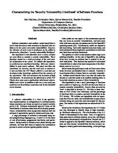
Fig. 4. (a) Schematic diagram of a baseline microprocessor. The two gray units are the structures under analyzing; (b) Reorder buffer entry [36].

program execution. The following equation describes how to compute a structure’s AVF through ACE bit analysis:

(2) where is the total bits in a hardware structure, is the execuis the number of ACE bits tion cycles of a program, and in the structure at a specific cycle . Another method to compute AVF is through statistical fault injection [30], [31]. Fault injection experiments are performed on a register transfer level (RTL) model of microprocessors. After injecting a fault, the architecture state of the fault injected simulator will be compared with a golden model to determine whether the injected fault results in an external error. After a huge number of fault injections, the percentage of faults leading to external errors is taken as AVF. Statistical fault injection is able to simulate any execution path and allows for high accuracy estimation. Most recently, Walcott et al. [32] use linear regression to identify the correlation between AVF and several key performance metrics (such as instructions per cycle and reorder buffer occupancy), and then use the predictive model to compute AVF dynamically during program execution. Duan et al. [33] propose an alternative prediction method to compute AVF across different workloads and microprocessor configurations using boosted regression trees and patient rule induction method. Prior works also demonstrate that AVF varies significantly and highly depends on microarchitecture structures and architecture programs [34]. In order to characterize the vulnerability of a program independent of microarchitecture structures, Sridharan et al. [18] propose PVF to evaluate the masking effect of soft errors at architecture level. They use A-bits (like ACE bits) and architecture resources (the structures which can be seen from the perspective of programmers, such as register file and arithmetic logic unit) to compute PVF. The equation to compute an architecture resource’s PVF can be expressed as follows:

(3)

where represents the total bits in the architecture resource, represents the total number of instructions in the program and represents the number of A-bits in instruction . PVF can be used to quantitatively estimate the masking effect of a program to soft errors and to express the behavior of AVF when executing a program. There are also several practical uses of PVF, such as choosing proper algorithms and compiler optimizations to reduce the vulnerability of a program to soft errors. Recently, Sridharan et al. [19] propose another metric HVF to analyze the vulnerability to soft errors only from microarchitecture level. AVF, PVF, and HVF, all of them are focusing on the masking effect of soft errors. Bower et al. [20] propose a metric named H-AVF for hard faults. H-AVF allows designers to compare alternative hard-fault tolerance schemes. For a given program, a structure’s H-AVF can be computed as (4) represents the total number of instructions in the prowhere represents the total number of fault sites in the strucgram, represents the number of instructions that will ture, and be corrupted due to hard faults. The purpose of H-AVF is to evaluate whether a particular sub-structure in microprocessors will benefit from hardening. It can also be used to compare hard-fault tolerance designs thus to provide a quantitative basis for comparison of alternative designs. Besides, Pellegrini et al. [35] propose a resiliency analysis system called CrashTest. CrashTest is capable of orchestrating and performing a comprehensive design resiliency analysis by examining how the design reacts to faults during program execution. This method mainly considers the impact of hard faults and soft errors on program execution. Unlike soft errors and hard faults, intermittent faults have many uncertain causes and their behaviors vary significantly. However, the vulnerability of microprocessor structures to intermittent faults is rarely considered. In this paper, we propose a metric IVF to characterize the vulnerability of microprocessor structures to intermittent faults. We compute IVFs for different microprocessor structures considering three intermittent fault models: intermittent stuck-at-1 and stuck-at-0 faults, intermittent open and short faults, and intermittent timing faults. III. IVF EVALUATION This section first describes our IVF evaluation algorithms for different intermittent fault models, and then presents the equations for IVF computation. A structure’s IVF is defined as the probability that an intermittent fault in the structure leads to an external visible error. The higher IVF, the more a structure is vulnerable to intermittent faults. In modern microprocessors, reorder buffer and register file are two of the most important hardware structures. Fig. 4(a) shows a baseline pipeline used in this work. Reorder buffer is used for out-of-order instruction execution, which allows instructions to be committed in-order. It keeps the information of in-flight instructions and allows for precise exceptions and easy rollback for control of target address mispredictions. The entry in reorder buffer is allocated in a round-robin order. Fig. 4(b) further shows typical fields contained in an entry of

This article has been accepted for inclusion in a future issue of this journal. Content is final as presented, with the exception of pagination. PAN et al.: CHARACTERIZING THE VULNERABILITY OF MICROPROCESSOR STRUCTURES TO INTERMITTENT FAULTS

reorder buffer [36]. These fields have different functions. The busy flag, issued flag, finished flag, speculative flag, and valid denotes the address of the flag are control signals, while current instruction, and rename register shows the renamed register for the destination register of an instruction. For register file, it is an array of processor registers and will be used to provide operation data during program execution. Each register in it contains 64 bits. If any of these two structures is affected by an intermittent fault, the probability resulting in a visible error is very high. We compute IVFs for these two representative structures in this work. Before IVF computation, the following two questions should be carefully answered. 1) How to determine whether an intermittent fault affects program execution? 2) In order to describe intermittent faults, how to set these three key parameters: burst length, active time, and inactive time appropriately? For the first question, to evaluate the impact of an intermittent fault on program execution, we need to determine whether the fault propagates to a storage cell and changes ACE bits during its lifetime. For intermittent stuck-at faults, as they only affect a single location, we should check whether the affected location contains an ACE bit, and then analyze whether the ACE bit is upset during the fault’s active time. Only the case when the affected location contains an ACE bit and the ACE bit is changed will affect program execution. For intermittent open and short faults, they may corrupt two adjacent bit lines. When such a fault occurs, we need to determine whether the fault propagates to a storage cell and change ACE bits. While for intermittent timing faults, they may cause timing violations and affect write operations. Only when an intermittent timing fault has been captured by a storage structure and changes ACE bits, it will affect program execution. For the second question, the parameters of an intermittent fault should follow the characteristics of an actual fault. As intermittent faults may be caused by different factors, the duration of intermittent faults could vary across a wide range of timescale. To set appropriate values for these key parameters, we analyze one kind of intermittent timing faults caused by significant voltage variation. The situation when supply voltage variation across a allowed voltage threshold is called a voltage emergency [37]. Voltage emergencies will lead to timing violations by slowing logic circuits. Fig. 5 shows an example of intermittent timing faults caused by voltage emergencies. As can be seen, intermittent timing faults caused by voltage variations usually last on the order of several to tens of nanoseconds. Prior works also show the similar duration of an intermittent fault [21]–[23]. According to the observation, we set the burst length of an intermittent fault in the range of 5 cycles to 30 cycles in our experiments. Both active time and inactive time are set to 2 cycles. The number of activations will be changed according to burst length, but the 50% duty cycle is kept constant. For an instance, if burst length is 30-cycle, the number of activations is 8. Besides, as the appearance time of intermittent faults cannot be predicted, their start time are randomly generated during program execution.

5

Fig. 5. Example of intermittent timing faults caused by voltage emergencies.

Fig. 6. ACE bits and un-ACE bits projection for IVF computing.

Based on the above analysis, the first step for IVF computing is to determine ACE bits in a structure during program execution; the second step is to check whether ACE bits are changed when an intermittent fault occurs. As reorder buffer is used to support out-of-order instruction execution, we analyze ACE bits in it by monitoring instructions when these instructions go through all stages of the pipeline. Meanwhile, register file is used to store and provide operation data for in-flight instructions, we analyze ACE bits in it based on its related operations, such as read, write, and evict. Following we present IVF computation algorithms for intermittent stuck-at faults, intermittent open and short faults, and intermittent timing faults, respectively. A. Intermittent Stuck-at Faults Intermittent stuck-at faults include intermittent stuck-at-1 faults and intermittent stuck-at-0 faults. As the analysis methods for these two kinds of faults are similar, for the sake of brevity, we take intermittent stuck-at-1 faults as an example in this section. 1) Reorder Buffer: We illustrate the IVF computation algorithm for reorder buffer at first. Unlike a soft error only existing for a single cycle, an intermittent fault will last for a while and repeatedly appear during its lifetime. Fig. 6 shows a 3-D perspective of a simplified reorder buffer. The -axis represents the number of entries in the structure, the -axis represents the number of bits in each entry, and the -axis represents the time of program execution. For the example structure, it has two entries and each entry contains two bits. The small black parallel-

This article has been accepted for inclusion in a future issue of this journal. Content is final as presented, with the exception of pagination. 6

Fig. 7. Lifetime of a register version with related operations. F , F , and F are three intermittent stuck-at faults occurring at different time.

ograms and white parallelograms are used to indicate ACE bits and un-ACE bits, respectively. For this example, we assume an intermittent stuck-at-1 fault occurs. The burst length is set to 2 cycles, while both active time and inactive time are 1 cycle. The gray part of the cube shows the possible affected region by the fault. The parallelograms in the - plane are planar representation of ACE bits and un-ACE bits for the gray part. For a specific bit, if it contains an ACE bit during the fault’s active time and its value is changed by the fault, the projection of that bit in - plane is an ACE bit, otherwise, the projection will be an un-ACE bit. As can be seen in Fig. 6, during the fault’s and contain ACE bits and will be affected active time, and contain ACE bits in the fault’s by the fault. Though inactive time, they will not be affected by the fault. To generate bit projection, we further need to analyze whether the values and will be changed. For the intermittent stuck-at-1 in fault, only if an ACE bit is supposed to be a logic value “0”, it and will actually be corrupted. Fig. 6 shows the values of during the active time. As the fault in-question is an intermittent stuck-at-1 fault, only the projection of is an ACE bit and other three bits are un-ACE bits. In this case, the probability that the fault leads to an external visible error is 25%, which means the IVF is 25%. With the above ACE bit analysis and bit projection, we can quickly determine whether an intermittent stuck-at fault affects program execution and further compute IVF for reorder buffer. 2) Register File: Unlike reorder buffer, the ACE bits analysis for register file is a little different. The ACE bits in register file are analyzed according to the related operations on each physical register. During the execution of a program, if the microprocessor decodes an in-flight instruction with a destination register, it will allocate a free physical register for the instruction, creating a new register version [38]. The lifetime of a register version is shown in Fig. 7. During the lifetime of a register version, the possible operations include allocation (A), write (W), read (R), and deallocation (D). A register version can only be written once but can be read several times during its lifetime. The lifetime of a register version is from allocation to deallocation and can be divided into three intervals: from allocation to ), and from write ( to ), from write to the last read ( to to ). Only the interval from the last read to deallocation ( write to the last read is critical time and other two intervals belong to noncritical time. During the critical time, all bits in the register are ACE bits. If an intermittent stuck-at-1 fault occurs during the critical time, these ACE bits with logic value “0” will be affected and lead to an external visible error (like fault ). If the fault occurs

IEEE TRANSACTIONS ON VERY LARGE SCALE INTEGRATION (VLSI) SYSTEMS

during noncritical time, it will always be masked (like fault ). A complicated situation is that a fault may start from a critical time region and end at a noncritical time region (like fault ). For this kind of fault, if its residency time in critical time region overlaps its active time, the fault can be handled like ; if there is no overlap, the fault will be masked. Only when an intermittent stuck-at-1 fault occurs during critical time and changes ACE bits will affect program execution. With the above analysis, the equation to compute IVF for reorder buffer and register file considering intermittent stuck-at faults can be expressed as

(5) represents the total number of bits in the structure where under analysis, represents a location in the structure, represents the burst length of an intermittent stuck-at fault, and represents whether an ACE bit in location will be changed by the fault; if it is, the value is assigned to one; otherwise, the value is assigned to zero. The numerator adds the total number of ACE bits that will be affected during the lifetime of an intermittent stuck-at fault. B. Intermittent Open and Short Faults Intermittent open and short faults have different behaviors depending on where they occur. They also can be taken as intermittent stuck-at faults or intermittent timing faults for some cases. Intermittent bridging faults, one kind of intermittent short fault, are different from intermittent stuck-at faults and intermittent timing faults. Intermittent bridging faults describe the cases when two signal wires are shorted together. They can be divided into four types: wired-AND, wired-OR, dominant-AND, and dominant-OR. For intermittent wired bridging faults, the logic value of the shorted nets is modeled as a logical AND or OR of the logic values on the shorted wires, while for intermittent dominant bridging faults, one wire is modeled to dominate the logic value on the shorted nets. The wired bridging faults were originally developed for bipolar circuits, while dominant bridging faults were for CMOS devices. Since CMOS technology is widely used for microprocessor manufacturing, we only analyze the dominant bridging faults in this work. An intermittent dominant bridging fault will corrupt two adjacent bit lines which produce two-bit of corruption. Fig. 8(a) and (b) show intermittent dominant-AND and dominant-OR bridging faults in the metal interconnect wires to reand are agorder buffer and register file, respectively. and are victim wires. The logic gressor wires, while value of the victim wire is dominated by the AND operation or OR operation of the logic value of the aggressor wire and its own value. For intermittent dominant-AND and dominant-OR faults, their controlling values are logic value “0” and logic value “1”, respectively. These two kinds of faults also have similar analysis methods, for the sake of brevity, we only take dominant-AND bridging faults as an example. The intermittent open and short faults refer to intermittent dominant-AND bridging faults if not specifically mentioned in the following analysis. When an intermittent dominant-AND bridging fault occurs, the value of the

This article has been accepted for inclusion in a future issue of this journal. Content is final as presented, with the exception of pagination. PAN et al.: CHARACTERIZING THE VULNERABILITY OF MICROPROCESSOR STRUCTURES TO INTERMITTENT FAULTS

7

Fig. 9. Intermittent timing fault results in writing a wrong data to a storage cell.

Fig. 8. Intermittent dominant-AND and dominant-OR bridging faults (a) in reorder buffer and (b) in register file.

victim wire will be changed only when the victim wire has a logic value “1” and the aggressor wire has a logic value “0”. The corrupted data of the victim wire then propagates during program execution. If the corrupt data propagates to a storage cell, we further need to determine whether the affected bit is an ACE bit or not. If it is an ACE bit, then the fault will result in an external visible error; otherwise, the fault is said to be masked. To compute IVFs of reorder buffer and register file for intermittent dominant bridging faults, we also need to analyze the data fields in them. As can be seen in Fig. 8(a), if the control bit in a reorder buffer entry has been corrupted, the instruction will be in a wrong state, and may lead to a fatal error. If the destination register tag is affected, the instruction result will be written to a wrong register. The bits in a register [shown in Fig. 8(b)], however, make no difference to the data if been affected, there is no need to further differentiate them. We only check the value containing in two adjacent lines and determine whether the fault changes ACE bits in that register. With the above analysis, the equation to compute IVF for reorder buffer and register file considering intermittent dominant bridging faults can be expressed as

(6) where represents the total number of intermittent domrepresents whether a fault propinant bridging faults, agates to reorder buffer or register file and finally affects ACE will set to one. Otherwise, will set to bits. If true, zero and the fault is said to be masked. C. Intermittent Timing Faults Unlike intermittent stuck-at faults which transform the correct value to a constant value, intermittent timing faults will affect data propagation and leads to capture wrong data to storage structure at entry level. Before present the algorithm to compute IVF for intermittent timing faults, we need to know when a fault will affect program execution. To determine the impact of an intermittent timing fault, two steps are needed: first, analyze whether the fault is captured by a storage cell; second, check whether ACE bits in the storage cell have been affected. Only when an intermittent

timing fault propagates to storage cells and changes ACE bits, it will affect the final program output. Otherwise, the fault will not manifest itself in external output and is said to be masked. In this work, we assume an intermittent timing fault only cause timing violations during its active time. If a write operation occurs during the active time of an intermittent timing fault, we assume the fault propagates to the structure. If no write operations occur or write operations only occur during inactive time, the fault is said to be masked and will not affect program execution. We use an example to further explain for this. Fig. 9 illustrates whether an intermittent timing fault will lead to capture a wrong data to a storage cell. As can be seen, write operation occurs during the active time of , the fault will propagate to a storage cell. While write operation occurs during the , the fault will not affect the data propainactive time of gation. With the above analysis, the frequency of write operations has strong correlation with the vulnerability of a structure to intermittent timing faults. During the lifetime of an intermittent timing fault, a structure with high write frequency is more vulnerable because the probability a fault propagating to the structure is very high. On the contrary, a structure with low write frequency is less vulnerable. To compute the IVF for different structures, we then need to determine whether a write operation is taken during the active time of an intermittent timing fault. For reorder buffer, the related write operations occur when the state of an instruction in it changes. For register file, the related write operations take place when an instruction commits or when a value is loaded from memory. The related write operations will be recorded for IVF computation during program execution. When a wrong data has been captured by a structure, we need to further analyze whether ACE bits in that cell have been changed by the fault. If ACE bits are upset, the fault will affect the external visible output. Otherwise, it is said to be masked at architecture level. There are mainly two scenarios that an intermittent timing fault will be masked during program execution: first, the data in a storage structure is proved to be a dead value; second, the captured data only changes un-ACE bits. If an intermittent timing fault is in either of the two scenarios, it will not affect program execution. Which scenario occurs is determined by analyzing ACE bits and un-ACE bits in different structures. For example, Fahs et al. [39] found that about 14% instructions are dead instructions during executing SPEC CPU2000 benchmarks. Dead instructions are those instructions whose results will not be used by any other instructions in the future. If the

This article has been accepted for inclusion in a future issue of this journal. Content is final as presented, with the exception of pagination. 8

IEEE TRANSACTIONS ON VERY LARGE SCALE INTEGRATION (VLSI) SYSTEMS

result of a dead instruction is changed by an intermittent timing fault, even if an incorrect data has been written to register file, the fault will not affect program execution. By analyzing ACE bits and un-ACE bits in different structures during program execution, we can determine which scenario occurs. Only an intermittent timing fault propagates to a storage cell and changes ACE bits, it will contribute to IVF computation. The equation to compute IVF considering intermittent timing faults can be expressed as

TABLE I SIMULATED MICROPROCESSOR CONFIGURATION

(7) where represents the total number of intermittent timing represents the number faults during executing a program; of intermittent timing faults propagating to the structure; represents the number of faults only affecting dead values; represents the number of faults only changing un-ACE bits. With this equation, we can compute for different microprocessor structures. D. Statistical Significance In this work, we use statistical sampling to study the characteristics of intermittent faults. To make the evaluation having statistical significance, a large number of faults should be analyzed during a simulation. After trying different number of faults, we set the fault number as 1000 to make a tradeoff between accuracy and analysis time. Besides, the burst length and the number of activations in an intermittent fault have significant impact on IVF computation. During executing different benchmarks, the two parameters will be changed to make our analysis more comprehensive, and the final IVF of a structure is the average result across all faults under analysis. With the above introduced (5)–(7), we can quickly compute IVFs for reorder buffer and register file. Furthermore, our proposed IVF estimation methodology also can be extended to other structures, such as issue queue, load/store queue, and L1/L2 caches. As the analysis of ACE bit in issue queue and load/store queue is also based on tracking the ACE bits in instructions when these instructions go through the pipeline, which is similar to the ACE analysis of reorder buffer. Besides, the analysis of ACE bit in L1/L2 caches is based on dividing the lifetime of a data block into critical time and noncritical time, which is similar to the ACE analysis of register file. Therefore, our IVF estimation methodology is also suitable for these structures. As all the above mentioned storage structures may occupy more than 60% area of modern microprocessors [40], our proposed evaluation methodology provides a generic metric for reliability estimation. IV. EVALUATION METHODOLOGY All of our experiments are conducted on the Sim-Alpha simulator [41]. Sim-Alpha is a validated execution-driven simulator for Alpha 21264 microprocessors [42]. It can execute instructions down the mis-speculated path, in the same way as an actual microprocessor would execute them. In this work, Sim-Alpha is heavily modified to support IVF computing for reorder buffer and register file. We use all the twelve SPEC

CPU2000 integer benchmarks to evaluate our method. Since the simulator cannot accurately simulate the floating-point pipeline, the floating-point benchmarks are not included in our experiments. All the benchmarks are compiled for the Alpha ISA. In order to reduce simulation time, we use Simpoint tool [43] to pick the most representative simulation point for each benchmark and each benchmark is fast-forwarded to its representative point before detailed performance simulation takes place. Each benchmark is evaluated for 100 million instructions using the full reference input set. The baseline configuration of the simulator is further summarized in Table I. As we focus on the integer pipeline, only the integer pipeline resources are shown in the table. Besides, to analyze the impact of different microarchitecture design parameters on IVF computation, we further change the number of fetch/slot/issue width, commit width, reorder buffer size, and register file size in our experiments. V. EXPERIMENTAL RESULTS In this section, we first present IVF of reorder buffer and register file considering different intermittent fault models, and then compute IVF by changing microarchitecture parameters and program phases. Finally, we introduce several IVF guided protection techniques to improve system reliability. A. IVF Computation for Different Intermittent Fault Models In our experiments, we compute IVF with different fault configurations by changing the key parameters of intermittent faults. The burst length of each intermittent fault is assigned to 6 cycles, 10 cycles, and 22 cycles, respectively. Both active time and inactive time are assigned to 2 cycles. The start time of each intermittent fault is randomly generated during program execution. 1) Intermittent Stuck-at Faults: For intermittent stuck-at faults, as the value of ACE bits will affect IVF evaluation, we in terms of intermittent stuck-at-1 fault model compute in terms of intermittent stuck-at-0 fault model, and respectively.

This article has been accepted for inclusion in a future issue of this journal. Content is final as presented, with the exception of pagination. PAN et al.: CHARACTERIZING THE VULNERABILITY OF MICROPROCESSOR STRUCTURES TO INTERMITTENT FAULTS

Fig. 10. Reorder buffer (left part) and register file (right part) AVFs considering soft errors and IVF

Fig. 11. Reorder buffer (left part) and register file (right part) IVF

Fig. 12.

IVF

9

considering intermittent stuck-at-1 faults.

considering intermittent stuck-at-0 faults.

for reorder buffer (left part) and register file (right part) considering intermittent dominant-AND bridging faults.

Figs. 10 and 11 show and for reorder buffer and register file during executing different benchmarks. The avfor reorder buffer and register file vary from 21% erage to 37% and from 21.4% to 31.5%, respectively. The average , however, vary from 5.8% to 10.3% and from 1.1% to 1.6%, respectively. As can be seen, the longer burst length, the more ACE bits been affected, which leads to a higher and . For a same burst length, the average is . This is because during executing difmuch higher than ferent benchmarks, the number of ACE bits containing logic value “0” is much more than these containing logic value “1”, especially in register file. ACE bits with logic value “0’ are vulnerable to intermittent stuck-at-1 faults, but not to intermittent and of restuck-at-0 faults. Meanwhile, both order buffer are much higher than that of register file. The reason is that the residency time of an instruction in reorder buffer is very long, from issue stage till commit stage. Register file, however, will be written very frequently, making its vulnerable time much shorter than that of reorder buffer. We also present the AVFs of reorder buffer and register file , their considering soft errors in Fig. 10. Compared to

AVFs are much lower. As an intermittent stuck-at-1 fault has longer duration than soft errors and most ACE bits contain logic value “0” in the two structures, which makes the probability an intermittent stuck-at-1 fault affecting final program execution is much higher. Therefore, intermittent stuck-at-1 faults have much more serious impact on program execution than soft errors if occur. The situation for intermittent stuck-at-0 faults, however, is just on the contrary. The reason is that soft errors can flip all the ACE bits while intermittent stuck-at-0 faults only affect these ACE bits with logic value “1”. 2) Intermittent Open and Short Faults: Fig. 12 shows for reorder buffer and register file considering intermittent dominant-AND bridging faults. As can be seen, for different burst length, the average for reorder buffer and register file vary from 14.8% to 23% and from 11.5% to 22.8%, respectively. These two structures have relatively low vulnerability to intermittent dominant bridging faults. When an intermittent dominant bridging fault occurs, only the case that the aggressor wire holds a controlling value and the victim wire holds a non-controlling value, the fault can propagate during program execution. With the same burst length, reorder buffer has a little higher

This article has been accepted for inclusion in a future issue of this journal. Content is final as presented, with the exception of pagination. 10

Fig. 13.

IEEE TRANSACTIONS ON VERY LARGE SCALE INTEGRATION (VLSI) SYSTEMS

IVF

for reorder buffer (left part) and register file (right part) considering intermittent timing faults.

than that for register file. The explanation is as follows: for reorder buffer, the control bits are more sensitive to intermittent dominant bridging faults; while for register file, however, it contains many narrow values during program execution. A value is categorized as narrow only if its leading bits are all zeros or ones. Kumar et al. [44] show about 50% of the produced results could be categorized as narrow values. For the narrow values in register file, they have higher masking rates to intermittent dominant bridging faults, which results in a lower . re3) Intermittent Timing Faults: We further present sults for reorder buffer and register file considering intermittent for reorder buffer and timing faults. Fig. 13 shows the register file during executing different benchmarks. As can be for reorder buffer and register file are seen, the average from 15.8% to 23.7% and from 19.7% to 30.6%, respectively. The longer burst length, the more write operations will be afresults. From Fig. 13, we fected, which leads to higher of register file is a little higher can tell that the average than that of reorder buffer, this is because register file provides operands for each instruction and has higher write frequency than reorder buffer. There is also a notable exception during executing two benchmarks gap and gzip. As for these two benchmarks, they have much higher cache miss rates than other benchmarks. During the time a cache miss occurs, the write operation for reorder buffer and register file will reduce dramatically, at that time. The widely which leads to a much lower used method to tolerate timing violations is to set a wider timing margin [45]. Only the intermittent timing faults occurring at critical paths and resulting in timing margin violation are what need to be considered. 4) Comparisons: Figs. 10, 12, and 13 have shown IVFs of reorder buffer and register file for three intermittent fault models. We then give a comparison of the impact of these faults. From these figures, it is easy to tell that intermittent stuck-at-1 faults have most serious impact on program execution during executing most benchmarks. For all these fault models, when the burst length of an intermittent fault increases, the probability to cause external errors is also increase, which means a structure’s IVF will increase. Besides, for a same fault model, the IVFs of reorder buffer and register file also vary significantly. Reorder buffer is more sensitive than register file to intermittent stuck-at faults and intermittent open and short faults, while less sensitive to intermittent timing faults. Utilizing the proposed IVF evaluation methodology, designers can quantitatively analyze the

masking effect of intermittent faults and guide system reliability design during the early design stage. In this work, we focus on the impact of intermittent faults, while Pellegrini et al.’s work CrashTest [35] analyzes the impact of hard faults and soft errors on program execution. Their experimental results shows that about 80% of stuck-at faults will cause errors, while only 40% of path-delay faults have adverse effects on program execution. Soft errors have the least impact on the correct functionally of the design and on average less than 10% of them cause an error. Comparing their results with our experimental results, it is easy to know that hard faults have most serious impact on program execution, followed by intermittent faults, and finally soft errors. Pellegrini et al.’s work combined with our work provides a global reliability picture for designers to understand the impact of different kinds of faults on program execution. B. IVF Computation for Different Microprocessor Configurations and Program Phases We have computed IVF for different intermittent fault models under a specified microprocessor configuration. In this subsection, we further extend our proposed methodology to address different microprocessor configurations. We choose four microarchitecture design parameters (fetch/slot/issue width, commit width, reorder buffer size, and register file size) which are believed to have impact on IVF computation. We change the size of these parameters to generate different microprocessor configurations. Tables II and III show four different microprocessor configurations for reorder buffer and register file, respectively. Of these configurations, rob_base and reg_base are the baseline configurations. We compute reorder buffer’s and register file’s IVF for each configuration shown in Tables II and III. Burst length is set to 10 cycles in the following experiments. Figs. 14–17 present our computed IVF results for different intermittent fault models. Each figure represents the result for one configuration. As can be seen, for configurations rob_c1 and reg_c1, reorder buffer’s and register file’s IVFs are much higher than the results of the baseline configuration. That is because when reduce a structure’s size, its occupancy increases greatly and the structure will be more vulnerable to intermittent faults. For configurations rob_c2 and reg_c2, on the contrary, the occupancy of a structure will reduce, which results in IVF reduction. While for configurations rob_c3 and reg_c3, though

This article has been accepted for inclusion in a future issue of this journal. Content is final as presented, with the exception of pagination. PAN et al.: CHARACTERIZING THE VULNERABILITY OF MICROPROCESSOR STRUCTURES TO INTERMITTENT FAULTS

11

TABLE II DIFFERENT MICROPROCESSOR CONFIGURATIONS FOR COMPUTING IVF OF REORDER BUFFER

TABLE III DIFFERENT MICROPROCESSOR CONFIGURATIONS FOR COMPUTING IVF OF REGISTER FILE

Fig. 14. Reorder buffer’s IVF on configuration rob_base (left) and register file’s IVF on configuration reg_base (right).

Fig. 15. Reorder buffer’s IVF on configuration rob_c1 (left) and register file’s IVF on configuration reg_c1 (right).

we reduce instruction fetch width and commit width, their IVFs also decrease significantly. This is due to both the number of in-flight instructions and the number of ACE bits in the pipeline reduces sharply during program execution. The experimental results reflect that a structure’s IVF varies across different microprocessor configurations and has high correlation with its size and the number of in-flight instructions. Besides, we can tell that intermittent stuck-at-1 faults have most serious impact while intermittent stuck-at-0 faults have minimal impact on program execution for most benchmarks. Our proposed IVF evaluation methodology can be easily extended to evaluate IVF for different microprocessor configurations and can be used to choose appropriate microarchitecture parameters during the early design stage. of reorder buffer and Furthermore, we compute register file for different program phases. All program phases are chose by Simpoint [43] and each contains 1 million inof reorder buffer structions. Figs. 18 and 19 show and register file during executing several benchmarks. As can be seen, IVF varies significantly across different program

phases and is heavily depended on the characteristics of a program. This phenomenon can be exploited to select proper protection techniques during program execution. We can use heavier protection (strict redundant multithreading) during highly vulnerable phases and lighter protection (partial or no redundant multithreading) during less vulnerable phases. With the dynamic tuning of protection, designers can achieve system reliability while minimize performance and/or energy overhead. The dynamic tuning of protection scheme also has been exploited to protect microprocessors from soft errors [32]. C. IVF Guided Reliable Design Our experimental results show that IVFs of reorder buffer and register file varies significantly, implying that these structures have different vulnerability to intermittent faults. Designers can exploit IVF information to determine which parts in microprocessors are most cost-effective to protect. For those structures with high IVFs, some heavyweight protection techniques are needed. We further introduce several possible techniques to improve system reliability.

This article has been accepted for inclusion in a future issue of this journal. Content is final as presented, with the exception of pagination. 12

IEEE TRANSACTIONS ON VERY LARGE SCALE INTEGRATION (VLSI) SYSTEMS

Fig. 16. Reorder buffer’s IVF on configuration rob_c2 (left) and register file’s IVF on configuration reg_c2 (right).

Fig. 17. Reorder buffer’s IVF on configuration rob_c3 (left) and register file’s IVF on configuration reg_c3 (right).

Fig. 18. IVF of reorder buffer for different program phases during executing twolf, vortex, and eon.

Fig. 19. IVF of register file for different program phases during executing mcf, crafty, and parser.

For intermittent stuck-at faults or intermittent open and short faults, a feasible protection scheme is to harden these high IVF structures with fault detection techniques (such as ECC or parity code). As intermittent faults occur in burst at the same location, if a fault in a storage cell has been detected for a predefined times, we can deduce that an intermittent fault has happened. At that time, a flag bit in the entry will be set to busy, and the entry will be unused for a while to avoid the influence of the intermittent fault. After then, the entry can be used again when the intermittent fault disappears, for example, when the power

delivery sub-system returns to its steady-state voltage. The partial protection technique ParShield proposed in [38] also can be used to protect register file from intermittent faults. Meanwhile, for intermittent timing faults, a prior proposed technique Razor [46] can be combined to these storage cells in critical paths of the most vulnerable structures, for example, Razor can be used to protect architecture registers as they are more vulnerable to intermittent timing faults. Besides, we can exploit architecture level masking of intermittent timing faults to improve system reliability [47]. The above introduced techniques seek to tolerate intermittent faults at fine-granularity. A coarse-granularity technique can be used to deal with intermittent faults in nowadays multi-core or many-core microprocessors. With inherent redundancy in these microprocessors, if a core sustains an intermittent fault, it should be suspended for a period of time, or operating system should transfer threads executing in the faulty core to other spare cores. Once the intermittent fault disappears later, the affected core can be used again. Besides, we also show that a structure’s IVF varies across different microprocessor configurations and program phases. This phenomenon can be exploited to select microarchitecture design parameters and tune protection schemes online. With the guide of IVF, designers can select appropriate protection techniques for these most vulnerable structures or program phases, which satisfies system reliability design goal while minimize implementation overheads. Nevertheless, combining our IVF evaluation methodology with these protection techniques is beyond the scope of this paper, we plan to exploit protection techniques to detect and recover from intermittent faults in our future work. VI. CONCLUSION Intermittent faults are emerging as a big challenge to reliable microprocessor design. In this paper, we propose a metric IVF to

This article has been accepted for inclusion in a future issue of this journal. Content is final as presented, with the exception of pagination. PAN et al.: CHARACTERIZING THE VULNERABILITY OF MICROPROCESSOR STRUCTURES TO INTERMITTENT FAULTS

quantitatively characterize the vulnerability of microprocessor structures to intermittent faults. The IVF evaluation methodology contains the following aspects: • analyze the physical causes of intermittent faults; • classify intermittent faults into different fault models based on their behaviors; • set key parameters for an intermittent fault and determine when the intermittent fault results in a visible error; • for a specific microprocessor structure, propose IVF computation algorithms for different intermittent fault models; • implement IVF computation algorithms in a high-level performance simulator, with which to compute IVF for the specific structure. With the IVF evaluation methodology, we compute IVFs for reorder buffer and register file in terms of intermittent stuck-at faults, intermittent open and short faults, and intermittent timing faults. Experimental results show that intermittent stuck-at-1 faults have most serious adverse impact on program execution among these three types of intermittent faults. Besides, IVF varies noticeably across different microprocessor structures and program phases. Our experimental results imply partial protection of the most vulnerable structures and program phases to enhance system reliability. With the guide of IVF evaluation methodology, we also discuss several possible intermittent fault detection and recovery techniques which can be used to improve system reliability. ACKNOWLEDGMENT The authors would like to thank the anonymous reviewers for their constructive comments. REFERENCES [1] J. W. McPherson, “Reliability challenges for 45 nm and beyond,” in Proc. Int. Des. Autom. Conf. (DAC), Jun. 2006, pp. 176–181. [2] C. Constantinescu, “Trends and challenges in VLSI circuit reliability,” IEEE Micro, vol. 23, no. 4, pp. 14–19, Jul./Aug. 2003. [3] T. Karnik, P. Hazucha, and J. Patel, “Characterization of soft errors caused by single event upsets in CMOS processes,” IEEE Trans. Depend. Secure Comput., vol. 1, no. 2, pp. 128–143, Jun. 2004. [4] C. Constantinescu, “Impact of deep submicron technology on dependability of VLSI circuits,” in Proc. Int. Conf. Depend. Syst. Netw. (DSN), Jun. 2002, pp. 205–209. [5] P. Wells, K. Chakraborty, and G. Sohi, “Adapting to intermittent faults in multicore systems,” in Proc. Int. Conf. Arch. Support for Program. Lang. Operat. Syst. (ASPLOS), 2008, pp. 255–264. [6] M. Kistler, S. Keckler, D. Burger, and L. Alvisi, “Modeling the effect of technology trends on soft error rate of combinational logic,” in Proc. Int. Conf. Depend. Syst. Netw. (DSN), 2002, pp. 389–398. [7] J. Srinivasan, S. V. Adve, P. Bose, and J. A. Rivers, “The impact of technology scaling on lifetime reliability,” in Proc. Int. Conf. Depend. Syst. Netw. (DSN), 2004, pp. 177–186. [8] C. Constantinescu, “Intermittent faults and effects on reliability of integrated circuits,” in Proc. Int. Symp. Reliab. Maintainability (RAMS), 2008, pp. 370–374. [9] T. J. Slegel, R. Averill, M. Check, B. Giamei, B. Krumm, C. Krygowski, W. Li, J. Liptay, J. MacDougall, T. McPherson, J. Navarro, E. Schwarz, K. Shum, and C. Webb, “IBM’s S/390 G5 microprocessor design,” IEEE Micro, vol. 19, no. 2, pp. 12–23, Mar./Apr. 1999. [10] A. Wood, “Data integrity concepts, features, and technology,” Tandem Division, Compaq Computer Corporation, TX, 1999. [11] S. Mukherjee, M. Kontz, and S. Reinhardt, “Detailed design and evaluation of redundant multithreading alternatives,” in Proc. Int. Symp. Comput. Arch. (ISCA), 2002, pp. 99–110. [12] T. Vijaykumar, I. Pomeranz, and K. Cheng, “Transient-fault recovery via simultaneous multithreading,” in Proc. Int. Symp. Comput. Arch. (ISCA), 2002, pp. 87–98.

13

[13] A. Parashar, S. Gurumurthi, and A. Sivasubramaniam, “SlicK: Slicebased locality exploitation for efficient redundant multithreading,” in Proc. Int. Conf. Arch. Support for Program. Lang. Operat. Syst. (ASPLOS), 2006, pp. 95–105. [14] S. Shyam, K. Constantiinides, S. Phadke, V. Bertacco, and T. Austin, “Ultra low-cost defect protection for microprocessor pipelines,” in Proc. Int. Conf. Arch. Support for Program. Lang. Operat. Syst. (ASPLOS), 2006, pp. 73–82. [15] SELSE, Urbana, IL, “SELSE workshop,” 2006 [Online]. Available: http://softerrors.info/selse/ [16] M. Li, P. Ramachandran, S. Sahoo, S. Adve, V. Adve, and Y. Zhou, “Understanding the propagation of hard errors to software and implications for resilient system design,” in Proc. Int. Conf. Arch. Support for Program. Lang. Operat. Syst. (ASPLOS), 2008, pp. 265–276. [17] S. Mukherjee, C. Weaver, J. Emer, S. Reinhardt, and T. Austin, “A systematic methodology to compute the architectural vulnerability factors for a high-performance microprocessor,” in Proc. Int. Symp. Microarch. (MICRO), 2003, pp. 29–40. [18] V. Sridharan and D. R. Kaeli, “Eliminating microarchitectural dependency from architectural vulnerability,” in Proc. Int. Symp. High Perform. Comput. Arch. (HPCA), 2009, pp. 117–128. [19] V. Sridharan and D. R. Kaeli, “Using hardware vulnerability factors to enhance AVF analysis,” in Proc. Int. Symp. Comput. Arch. (ISCA), 2010, pp. 461–472. [20] F. Bower, D. Hower, M. Yilmaz, D. Sorin, and S. Ozev, “Applying architecture vulnerability analysis to hard faults in the microprocessor,” in Proc. ACM SIGMETRICS/Perform. (Poster Session), Jun. 2006, pp. 375–376. [21] J. Smolens, B. Gold, J. Hoe, B. Falsafi, and K. Mai, “Detecting emerging wearout faults,” presented at the Workshop Silicon Errors in Logic—Syst. Effects (SELSE), Austin, TX, 2007. [22] J. Gracia, L. Siaz, J. Baraza, D. Gil, and P. Gil, “Analysis of the influence of intermittent faults in a microcontroller,” in Proc. Int. Workshop Des. Diagnostics Electron. Circuits Syst. (DDECS), 2008, pp. 1–6. [23] J. H. Stathis, “Physical and predictive models of ultrathin oxide reliability in CMOS devices and circuits,” IEEE Trans. Device Mater. Reliab., vol. 1, no. 1, pp. 43–59, Mar. 2001. [24] D. Gil, J. Gracia, J. Baraza, and P. Gil, “Study, comparison and application of different VHDL-based fault injection techniques for the experimental validation of a fault-tolerant system,” Microelectron. J., vol. 34, no. 1, pp. 41–51, Jan. 2003. [25] L. Wang, C. Wu, and X. Wen, VLSI Test Principles and Architectures Design for Testability. Boston, MA: Morgan Kaufmann, 2006. [26] J. Srinivasan, S. Adve, P. Bose, and J. Rivers, “Exploiting structural duplication for lifetime reliability enhancement,” in Proc. Int. Symp. Comput. Arch. (ISCA), 2005, pp. 520–531. [27] S. Borkar, T. Karnik, S. Narendra, J. Tschanz, A. Keshavarzi, and V. De, “Parameter variations and impact on circuits and microarchitecture,” in Proc. Int. Des. Autom. Conf. (DAC), 2003, pp. 338–342. [28] A. Biswas, P. Racunas, R. Cheveresan, J. Emer, S. Mukherjee, and R. Rangan, “Computing architectural vulnerability factors for addressbased structures,” in Proc. Int. Symp. Comput. Arch. (ISCA), 2005, pp. 532–543. [29] X. Fu, T. Li, and J. Fortes, “Sim-SODA: A unified framework for architectural level software reliability analysis,” presented at the Workshop Model., Benchmark., Simulation (MoBS), Boston, MA, 2006. [30] N. Wang, J. Quek, T. Rafacz, and S. Patel, “Characterizing the effects of transient faults on a high-performance processor pipeline,” in Proc. Int. Conf. Depend. Syst. Netw. (DSN), Jun. 2004, pp. 61–70. [31] E. Touloupis, J. Flint, V. Chouliaras, and D. Ward, “Study of the effects of SEU-induced faults on a pipeline-protected microprocessor,” IEEE Trans. Comput., vol. 56, no. 12, pp. 1585–1596, Dec. 2007. [32] K. R. Walcott, G. Humphreys, and S. Gurumurthi, “Dynamic prediction of architectural vulnerability from microarchitectural state,” in Proc. Int. Symp. Comput. Arch. (ISCA), 2007, pp. 516–527. [33] L. Duan, B. Li, and L. Peng, “Versatile prediction and fast estimation of architectural vulnerability factor from processor performance metrics,” in Proc. Int. Symp. High Perform. Comput. Arch. (HPCA), 2009, pp. 129–140. [34] S. Pan, Y. Hu, and X. Li, “Online computing and predicting architectural vulnerability factor for microprocessor structures,” in Proc. Pacific Rim Int. Symp. Depend. Comput. (PRDC), 2009, pp. 345–350. [35] A. Pellegrini, K. Constantinides, D. Zhang, S. Sudhakar, V. Bertacco, and T. Austin, “CrashTest: A fast high-fidelity FPGA-based resiliency analysis framework,” in Proc. Int. Conf. Comput. Des. (ICCD), 2008, pp. 363–370.

This article has been accepted for inclusion in a future issue of this journal. Content is final as presented, with the exception of pagination. 14

IEEE TRANSACTIONS ON VERY LARGE SCALE INTEGRATION (VLSI) SYSTEMS

[36] J. Shen and M. Lipasti, Modern Processor Design: Fundamentals of Superscalar Processors (Beta Edition). New York: McGraw Hill, 2003. [37] R. Joseph, D. Brooks, and M. Martonosi, “Control techniques to eliminate voltage emergencies in high performance processors,” in Proc. Int. Symp. High Perform. Comput. Arch. (HPCA), 2003, pp. 79–90. [38] P. Montesinos, W. Liu, and J. Torrellas, “Using register lifetime predictions to protect register files against soft errors,” in Proc. Int. Conf. Depend. Syst. Netw. (DSN), 2007, pp. 286–296. [39] B. Fahs, S. Bose, M. Crum, B. Slechta, F. Spadini, T. Tung, S. Patel, and S. Lumetta, “Performance characterization of a hardware mechanism for dynamic optimization,” in Proc. Int. Symp. Microarch. (MICRO), 2001, pp. 16–27. [40] B. Stackhouse, B. Cherkauer, M. Gowan, P. Gronowski, and C. Lyles, “A 65 nm 2-billion transistor quad-core itanium processor,” in Proc. Int. Solid-State Circuits Conf., 2008, p. 92. [41] R. Desikan, D. Burger, S. Keckler, and T. Austin, “Sim-alpha: A validated, execution-driven Alpha 21264 simulator,” Dept. Comput. Sci., Univ. Texas, Austin, Tech. Rep. TR-01-23, 2001. [42] R. E. Kessler, “The Alpha 21264 microprocessor,” IEEE Micro, vol. 19, no. 2, pp. 24–36, Mar./Apr. 1999. [43] T. Sherwood, E. Perelman, G. Hamerly, and B. Calder, “Automatically characterizing large scale program behavior,” in Proc. Int. Conf. Arch. Support for Program. Lang. Operat. Syst. (ASPLOS), 2002, pp. 45–57. [44] S. Kumar and A. Aggarwal, “Reducing resource redundancy for concurrent error detection techniques in high performance microprocessors,” in Proc. Int. Symp. High Perform. Comput. Arch. (HPCA), 2006, pp. 212–221. [45] M. Annavaram, E. Grochowski, and P. Reed, “Implications of device timing variability on full chip timing,” in Proc. Int. Symp. High Perform. Comput. Arch. (HPCA), 2007, pp. 37–45. [46] D. Ernst, N. Kim, S. Das, S. Pant, R. Rao, T. Pham, C. Ziesler, D. Blaaw, T. Austin, K. Flatner, and T. Mudge, “Razor: A low-power pipeline based on circuit-level timing speculation,” in Proc. Int. Symp. Microarch. (MICRO), 2003, pp. 7–18. [47] S. Pan, Y. Hu, X. Hu, and X. Li, “A cost-effective substantial-impactfilter based method to tolerate voltage emergencies,” in Proc. Int. Conf. Des., Autom., Test Eur. (DATE), 2011, pp. 311–316. Songjun Pan (S’10) received the B.S. degree in computer science from Huazhong University of Science and Technology, Hubei, China, in 2006. He is currently pursuing the Ph.D. degree in computer science from the Institute of Computing Technology, Chinese Academy of Sciences, Beijing, China. His research interests include reliability modeling and fault-tolerant design.

Yu Hu (M’06) received the B.S., M.S., and Ph.D. degrees from University of Electronic Science and Technology of China, in 1997, 1999, and 2003, respectively, all in electrical engineering. She is currently an Associate Professor with the Institute of Computing Technology, Chinese Academy of Sciences, Beijing, China. Her research interests include reliable design, fault diagnosis, and multiprocessor testing. Prof. Hu was a member of ACM, IEICE, and CCF.

Xiaowei Li (SM’04) received the B.Eng. and M.Eng. degrees in computer science from Hefei University of Technology, Hefei, China, in 1985 and 1988, respectively, and the Ph.D. degree in computer science from the Institute of Computing Technology (ICT), Chinese Academy of Sciences (CAS), Beijing, China, in 1991. From 1991 to 2000, he was an Assistant Professor and an Associate Professor (since 1993) with the Department of Computer Science and Technology, Peking University, Beijing, China. He joined the ICT, CAS as a Professor in 2000. He is now the deputy director of the Key Laboratory of Computer System and Architecture, CAS. His research interests include VLSI testing, design for testability, design verification, dependable computing, and wireless sensor networks. He has copublished over 150 papers in academic journals and international conference, holds 21 patents, and 29 software copyrights. Dr. Li serves as chair of Technical Committee on Fault Tolerant Computing, China Computer Federation (CCF) since 2008. He serves as vice chair of IEEE Asian Pacific Regional Test Technology Technical Council (TTTC) since 2004. He serves as the steering committee vice-chair of IEEE Asian Test Symposium since 2007. He also served as the steering committee chair of IEEE Workshop on RTL and High Level Testing. In addition, he serves on the Technical Program Committee of several IEEE and ACM conferences, including VTS, DATE, ASPDAC, PRDC, etc. He also serves as member of editorial board of JCST, JOLPE, JETTA, etc.