J1.1
EVALUATION OF SENSOR PLACEMENT TECHNIQUES Ian Griffiths*, Martyn Bull and Ian Bush RiskAware Ltd, Bristol, UK
1.
INTRODUCTION
Sensors for detecting toxic airborne materials are important assets that can be expensive and often limited in availability. Chemical and biological (CB) sensors need to be positioned with care to provide the maximum information to allow timely identification of an accidental or intentional release of dangerous materials. The aim is to minimise the casualties and effects, and this should be the key goal of any placement strategy. This application is of particular relevance to homeland security and defence applications where there is a need to put in place protective measures. There are placement: 1.
2.
two
main
approaches
to
sensor
Rules-based sensor placement in which sensors are placed according to heuristic rules. This approach is particularly appealing to the military as it provides a set of rules that can be followed consistently and which can be described by doctrine. Computational optimisation, which involves running multiple dispersion simulations and then using an optimiser to determine the best placement. This approach can be computationally intensive, and so it is possible that its application may need to be reserved for special cases. We are interested to determine whether techniques can be developed that enable a rapid computer-based capability to be produced that can be used in operational circumstances.
In this study we have implemented and compared the two approaches. Our aim was to determine the relative benefits of rules-based and computer optimisation, and how these approaches may be improved in the future. 2.
TECHNICAL DETAILS
military base). By treating it as an optimisation problem it is possible to develop computer-based capabilities that will automatically identify the best sensor locations against user-defined identify the best sensor locations against user-defined goals and within user-specified constraints. It is expected they can automatically provide placement solutions that trade off probability of detection and warning time. We have implemented a computer optimisation approach called SPARTA (Sensor Placement Algorithm for Rapid Theatre Assessment), which we will use in this evaluation study. Figure 1 provides an overview of the SPARTA inputs, data processing and optimisation. The tool takes in as inputs: •
Domain information, including the location and extent and information on the population (or other entities that are to be protected), as well as the desirability of different locations for placing sensors (e.g. it may not be possible to place them in a lake).
•
Information on the materials to be considered, in particular the toxicity of the agents.
•
Threat information, including distributions for potential release locations, the sizes and masses of releases, and the materials that may be released for the particular threat.
•
Sensor information, including the numbers and types of sensors and how they respond to different agents that are being considered (including threshold levels and response times).
•
Meteorological information, such as climatological data for a location for long-term deployment or weather forecast data for a short-term placement.
•
Mitigation options, such as medical treatment or, in the case of the military, wearing of individual protective equipment (IPE) such as respirators.
2.1 Computerised Sensor Placement Optimisation CBRN sensors are a limited resource and their placement needs to be optimised to provide the most useful information. The highest priority placement consideration is generally likelihood of detecting a release, but another important factor is warning time (the duration from determining an event has occurred to the agent reaching the assets to be protected, such as a * Corresponding author address: Ian Griffiths, RiskAware Ltd, Colston Tower, Colston Street, Bristol BS1 4XE, UK; e-mail:
[email protected].
Figure 1: SPARTA computation process.
In SPARTA it is possible to describe the input in detail, for example a detailed wind rose for the meteorological input or a grid of release location probabilities for the threat. Alternatively simple definitions can be used, such as a wind direction and variability estimate or a threat target area described as a simple geometric shape. This provides a great level of flexibility. SPARTA has two main stages in its computation approach: •
First, a store of possible event simulations are computed – this may be many thousands of different runs with varying conditions such as release parameters (material, mass and location), wind speed and direction, etc. Because the aim of the placement is to minimise the damage caused by a CB event, which is usually taken as the number of casualties, although it could be defined in alternative ways, SPARTA actually calculates the casualties for each scenario. It uses a separate transport and dispersion model, by default a very rapid model we have developed for this purpose although this could be replaced by a more sophisticated modelling capability if required.
•
Second, an optimiser is used to calculate the best locations for the sensors by comparing the results for placing different combinations of sensor location within each challenge of the sampled simulated scenarios. Currently a sequential optimiser is used as follows: 1.
For each location in the domain, SPARTA calculates the reduction in casualties that would be achieved on average for all the calculated challenges by placing a sensor at that position.
2.
As SPARTA is effects based, this could be either wearing IPE or having medical treatment (or whatever other mitigation is available for use). These provide very different results and SPARTA calculates all the different outcomes from using the available mitigation options given the placement of the sensor.
3.
SPARTA places the sensor at the location that provides the greatest overall casualty reduction.
4.
The challenge effects memory store is then updated to reflect the reduction of casualties across each challenge that was achieved by the newly placed sensor. SPARTA then removes all those challenges where the sensor placement will have reduced the casualties below a threshold.
5.
The sequential optimiser returns to step 1 and repeats the process with the next sensor until
all sensors are placed, all the casualty reduction offered by placing the sensor is below a threshold (generally set to 1 person). The outputs provided by SPARTA are numerous but include: a list of sensor locations, an estimate of the casualty reduction that will be provided by the locations (given for each additional sensor placed), estimates of remaining areas of highest concern, and more. It should be noted that SPARTA automatically handles the distinction between chemical and biological scenarios. Chemical sensors have a fast response time, generally in order of seconds, while the time to onset of effects for chemical agents is very rapid (tens of seconds). This means that the use of IPE offers the best protection strategy, and as it can take ten or more seconds for military personal to don a respirator, it is crucial that sensors are placed sufficiently upwind to detect the dispersing agent and provide enough warning time. For biological releases, the onset of symptoms can be several days but for many agents treatment can be successfully administered for several hours, e.g. up to a day. It is therefore imperative that sensors are placed to maximise the probability of detection as then personnel can be treated. As biological sensors are generally slow to provide a definitive identification of an agent (several hours), it is not feasible to detect the biological agent before it has passed the area being protected, which emphasises the priority of maximising the probability of detection. Because SPARTA minimises effects it automatically handles these different priorities: it maximises warning time against chemical threats and maximises probability of detection for biological threats. The main challenge to automated sensor placement is computation time. To be robust, the optimisation requires many simulations because of the range of possible event scenarios and conditions and the need to ensure sufficient coverage of these using Monte Carlo sampling. Much of the development of SPARTA has focused on methods for handling the large numbers of simulations efficiently when optimising. This has been achieved by creating a multi-level cache. Modelled dispersion results are stored and re-used wherever possible. This includes manipulation of plumes for different release masses and wind directions. The second stage cache stores the calculated effects, which allows these expensive computations to be reused. It should be noted that this data store of dispersion and effects is built up during operation (generally very rapidly through several executions of the tools), and it is not necessary to install a large data set of pre-run results. This does raise the question of how many Monte Carlo samples are required to provide a reliable placement. Figure 2 provides the effectiveness in terms of percentage casualty reduction for a range of different scenarios with increasing numbers of samples. It can be seen that the effectiveness levels off in each case (although at different levels). In some cases, this has
the behaviour we would expect as the sensors are being placed to maximise warning time, which is the key criteria for successful chemical sensor placement. As the areas begin to overlap, we see that the sensors are distributed fairly evenly throughout the overlap region, no matter what the wind direction is.
Figure 2: Effect of sample size for chemical threats (using ten sensors) and biological scenarios (using four sensors). Four sets of input meteorology data: uniform wind speed and direction (the greatest challenge), variable met generally from the SW, more complex met, and a simple wind distribution.
The biological case is very different to the chemical case when there is a predominant wind direction. The algorithm consistently places the sensors at the downwind edge of the domain, even if there is an overlap of the threat and protection areas. This will maximise the probability of detection – the key to successful biological sensor placement – as the hazard plumes will spread laterally as it disperses and so, within the sensor threshold limit, more plumes can be detected further downwind. It can be seen that some sensors are placed further upwind, this is when SPARTA has placed sensors to detect most of the challenge plumes, if it can place the final ones to maximise warning time while detecting the hazard even
levelled off by about 1,000 samples although in others it takes 5,000 or even more samples. (The reason for the high effectiveness with very low numbers of samples is that there is a high sensor to sample ratio, which makes it easy to place the sensors to capture the threats.) It is possible that a relationship could be found between the complexity of the scenario and the number of samples required and this will be investigated further. However, throughout this evaluation we have used 5,000 samples, which we feel is sufficient. Typically SPARTA is able to perform a placement using 5,000 samples in about 20 minutes (with 3,000 typically taking 15 minutes and 1,000 taking less than 10 minutes). Sample Test Cases of Automated Sensor Placement Several test cases were investigated to enable a basic evaluation of the SPARTA placement in simple and highly controlled scenarios. They also provided an understanding of the computer-based optimisation strategy. More than 140 scenario variations were investigated and only a few of them are discussed here. Figure 3 provides the results of the SPARTA optimal placement of chemical sensors for idealised rectangular threat and protection areas, and Figure 4 is for the same cases but with biological releases. In both sets, diagrams a to d show the effects of reducing the separation of the threat and protection areas when there is a westerly wind. We can also compare the effects of wind direction in cases a and c, where there is the westerly wind, with e and f, respectively, where there is a uniform wind. In the chemical case we can see that the sensors are placed between the protection and threat areas and when there is a separation, the gap between them is filled. This is true whether the wind comes from the west only or is sampled from a uniform distribution. This is
Figure 3: Optimal placement of 20 chemical sensors (blue markers) for rectangular threat areas (pink dots show release locations) and rectangular protection areas (in grey) with varying separation distances. a to d have westerly winds; e and f have uniform winds.
Figure 4: Optimal placement of 8 biological sensors (red markers) for rectangular threat areas (pink dots show release locations) and rectangular protection areas (in grey) with varying separation distances. a to d have westerly winds; e and f have uniformly distributed wind. in the biological case, it will do so. The results for the wind direction sampled from a uniform distribution are completely different and in fact very similar to the chemical case – the sensors are placed to fill any gap or spread evenly across an overlap. This is because plumes could be passing across the protection area at various angles, just clipping the edges in some cases – to maximise the probability of detection in this case the sensors need to be placed nearer to the threat. Figures 5 and 6 show chemical and biological sensor placements, respectively, for a circular protection area surrounded by a threat ring, which grows in width until it touches and then engulfs the protection. In each case, the figures on the left (a, c and e) have a wind direction from the west, whereas those on the right (b, d and f) have the wind direction uniformly distributed. (It may be observed that the threat area appears skewed towards the upwind direction; this is because SPARTA ensures its hazard samples all interact with the protection area, as those plumes that do not affect personnel do not need to be detected in order to protect
Figure 5: Optimal placement of 20 chemical sensors (blue markers) for circular threat areas (pink dots show release locations) and circular protection areas (in grey) with varying separation distances. a, c and e have wind from West; b, d and f have uniformly distributed wind.
the population and so are ignored.) There are similarities with the rectangular cases. If there is a predominant wind direction, for the chemical scenarios the sensors are placed upwind if there is no overlap of the threat and protection areas, otherwise the sensors are spread throughout the overlap; whereas for the biological scenarios they are always placed far downwind to maximise the probability of detection. Where the wind is uniformly distributed, the sensors, both chemical and biological, are spread throughout the protection area. 2.2 Rules-based Sensor Placement For this evaluation, we implemented a number of rules-based methods that place sensors against prescribed rules. These include some commonly used rules and some more sophisticated ones developed based on the results of the sample test cases carried out using the automated optimisation techniques, such as those examples described above.
military approach), which was proposed by Griffiths (2009) as an improvement over Rule 1. The third and fourth rules are inspired by the SPARTA test case results: Rule 3 is based on a simple interpretation whereas Rule 4 is based a more sophisticated analysis of the results. However, in Rule 4 the wind direction for the biological case is deliberately ignored (as this makes the rule simpler for general application) so the resulting rule attempts to provide a compromise between the meteorological cases. All of the above rules can be implemented manually, which is the appeal for some operational applications. However, they are readily implemented as algorithms to be executed on a computer and we have implemented them for this study. We use a simulated annealing algorithm to automate the even spreading of sensors within areas. 3.
STUDY DETAILS The evaluation study used two approaches:
Figure 6: Optimal placement of 8 biological sensors (red markers) for circular threat areas (pink dots show release locations) and circular protection areas (in grey) with varying separation distances. a, c and e have wind from West; b, d and f have uniformly distributed wind. The rules we have considered are: 1.
Place the sensors evenly around the perimeter of protection area.
2.
Spread the sensors protection area.
3.
If the threat and protection areas do not overlap, place the sensors evenly around perimeter of the protection area; otherwise spread them evenly throughout protection area.
4.
evenly
throughout
the
For chemical, if the threat area and protection area do not overlap, place evenly around the part of the perimeter that faces the threat area; otherwise spread them throughout the overlap area. For biological, always place on perimeter of the protection area.
The first rule is a common doctrinal rule. The second rule is similar to the Dice-5 placement strategy for five sensors repeated across an area (this is also a
•
High level (lower fidelity) simulation runs. This employs a simple modelling approach that allows large numbers of Monte Carlo sampled scenario variations to be carried out
•
Low level cases for treatment using highly detailed (high fidelity) simulation techniques. This more advanced approach allows a more detailed analysis but as it is more computationally intensive less simulations are considered.
The capability for carrying out both approaches is part of an evaluation system for conducting evaluation studies. For both approaches, two different domains and challenge scenarios sampled from the same underlying distributions were used. The high level modelling considered 50 different scenarios with 5,000 simulation repeats for each. The highly detailed cases consider the same 50 separate scenarios sampled between 10 and 20 times each. The performances of the various sensor placement techniques for the same challenges were then compared. Griffiths (2009) described the use of field trials data, namely the FUSION Field Trial 2007 (FFT07) data set, although this has not yet been revisited for this evaluation. 3.1 Challenge Generation The high level approach uses rapid modelling of each scenario and providing results data that allows the calculation of evaluation metrics, in this study the number of casualties. The modelling uses simplified representations that capture the main aspects of the physics and processes involved, including Gaussian dispersion modelling for the transport and diffusion, response and effects, and the statistics of the results. Thousands or even millions of simulations can be modelled automatically by the system in a matter of days and all the output collated.
The highly h detailed modelling uses an advancced synthetic environment that t has bee en developed to produce challenge c data a for evaluattion studies. As described by Bull (2009), the core component is a physics-ba ased concentrration fluctuattion model th hat produces realistic conce entration time series with the t appropriate e complex structure and whicch, importantly,, is correlated in space an nd time. It ta akes as input a concentration ensemble mean, varia ance and leng gth scale field (as produced by, for examp ple, the SCIPUFF dispersion model). The e synthetic environment also includes se ensor models and a various hu uman effects and a performancce models, physiological burrden models and a mitigation response mod dels. In this way w the synthe etic environment can be used d to create cha allenge data se ets which can be used for test and evalu uation as in this study. Figu ure 7 provides an example e of a simulatted concentration realisation field produced d by the syste em. By integrrating these instantaneouss concentratiion realisation fields over the simulattion duration a challenge dosage can be calculated d and from this casualty esstimates produ uced for the diifferent mitigatiion responses available. The e casualty esttimates can th hen t different se ensor placeme ent be comparred between the approaches, which are ea ach challenged d in turn.
Figure 8: Bagram airr force base with w release loccations (in red)) showing threa at areas: A – uniform distributtion, B – Gausssian distributio ons over key arreas of the basse, C – single Gaussian G distrribution centred d on base enttrance, and D – Gaussian distributions representing r re elease nsurgents. capacitty of possible in al sensors we ere available,, with and eight biologica permitte ed locations within the ba ase perimeterr. The sensor deployments were w defined ass:
A example con ncentration rea alisation field with w Figure 7: An modelled sensor s alarm status (yellow w – non-alarme ed, red – alarm med).
1.
Ind definite – the se ensors will be placed out to protect p the e based as a matter of course. There is no spe ecific informattion on the th hreat so a uniform disstribution is use ed (A). Annuall climatology iss used as the weather in nput.
2.
s Long term – there sensors are deployed for several mo onths over Win nter. There is a belief that the e base ma ay be targeted so the threat distribution d is fo ocused on this (B). The e climatology data for the winter onths was used d for the meteo orology. mo
3.
edium term – there is in ntelligence tha at the Me enttrance to the e base may be targeted in i the folllowing month, July (C). The climatology weather forr July is used.
4.
Sh hort term – there are reports that insurgentts may attack using mo ortars or from hand held devices from the north ea ast and so a possible p threat profile is produced p (D). The T 5 day wea ather forecast iss used as the meteorolog gical input.
3.2 Descrription of Evalluation Scenarrios Two sets of scenario os were used: one for a milita ary base in Affghanistan and the other for a city in the UK. U Throughou ut the study ca are was taken to ensure it was w completelyy unclassified and no classsified informatiion was used. Populations were estimatted from openly available imagery, i mete eorological datta was obtain ned from uncla assified sources or from crea ated distribution ns, and senso or and agent properties were e also taken fro om unclassified sources or plausible value es were used. It should be emphasised th hat all threat scenarios s used in d by the autho ors and are not n the study were devised derived from official inform mation or previious work. The firrst set of scenarios used foccused on Bagra am air force ba ase in Afghanis stan – Figure 8. 8 A 5 km doma ain was used that t encapsulatted the base. Twenty T chemical
The second set of scenarios used u were bassed in s Bristol, UK – Figure 9. It consistss of a 5 km square n that includes most of the central area of th he city. domain Here th he sensor dep ployments considered were based on pro otecting against combinatio ons of threatss and
Figure 9: Bristol showing release locations (in red) and threat areas: A – College Green, B – Queen’s Square, C – dispersed threat area, and D – River Avon. deployment duration, which affected the meteorological conditions. Again there were twenty chemical and eight biological sensors available for placement. The challenge scenarios for Bristol were defined by: •
Four threat location distributions – one focused on a open space in front of the local government headquarters (A), another in a square in a commercial area (B), a third widely dispersed but centred in the city centre (C) and the fourth along the river route into the city (D).
•
Five meteorological distributions represented by wind roses of the annual meteorology for Bristol, two climatology data sets for two separate months, a three day weather forecast and a totally uniform meteorological distribution.
Figure 10: Example SPARTA optimised placement of 20 chemical sensors (blue) – short term deployment case. For the high-level analysis runs, the Evaluation System sampled 5,000 individual challenge scenarios for each of the 48 main test scenarios (4 for each of chemical and biological for Bagram and 20 for both agent types for Bristol). SPARTA and the four rulesbased placements were then evaluated using these challenges. For each test scenario the average reduction in casualties were calculated based on available mitigation in response to modelled sensor response for the placements.
This resulted in 20 different combinations, and for each of these chemical and biological releases were considered. Figure 9 shows the release locations used in the high-level challenge evaluation. 4.
RESULTS
SPARTA was first run for all the different test cases. Two examples of SPARTA generated sensor deployments for these operationally realistic scenarios are shown in Figures 10 and 11. Each of these was produced in a run time of approximately 15 minutes. The implementations of the four rules based approaches were then used to produce rules based placements.
Figure 11: Example SPARTA optimised placement of eight biological sensors (red) – river based threat and forecast meteorological input (generally SW wind).
The results of the high-level analysis are shown in Figure 12. We can see that SPARTA performs better than all four rules-based methods in almost all scenarios, and in those cases where it does not outperform the results are near identical. Although it is clear from the figure that SPARTA is performing the best, the differences in the results for the rules approaches are not obvious. Table 1 provides a summary of the comparative ranks for all the approaches. This confirms that SPARTA outperforms all the rules-based approaches in more than 95% of the scenarios.
diagonal line (a measure of it getting closer to the performance of SPARTA) except in four cases, where it performs poorly. All of these cases relate to the same threat distribution: a chemical release in Queen Square (B of Figure 9). If one looks at the performance excluding this threat case (see Table 2), it can be seen that Rule 4 performs the best of all the rules. The Queen Square threat area is highly localised and reviewing Rule 4, one can see that for chemical the sensors will be placed in the overlap area of the threat and protection areas, which will be small. Although Rule 4 generally performs well, it is likely that it requires some modification to better handle localised threat areas to improve it robustness, by perhaps adding a buffer zone around the overlap to extend it. Average casualty reduction
SP
R1
R2
R3
R4
80.4%
66.3%
68.9%
69.3%
70.7%
Table 2: High-level analysis average percentage casualty reductions for SPARTA (SP) and Rules 1 to 4 (R1-R4) in which Queen Square threat has been excluded.
Figure 12: Results of the high-level analysis – comparisons between SPARTA placements and rulesbased placements. Points in the area below the diagonal line indicate cases SPARTA performed better.
Rank 1 2 3 4 5 Average rank Average casualty reduction
SP 46 0 1 1 0
R1 1 5 8 16 13
R2 0 13 12 11 11
R3 0 14 17 10 7
R4 1 16 10 10 9
1.1
3.4
3.5
3.2
3.1
81.3%
65.0%
69.3%
69.5%
64.8%
Table 1: High-level analysis rankings and average percentage casualty reductions for SPARTA (SP) and Rules 1 to 4 (R1-R4). In terms of rank, Rule 3 performs the next best although all the rules provide similar levels of protection. However, when one examines the average percentage of casualty reduction across all the scenarios, it can be seen that Rule 4 offers the least protection, very similar to Rule 1 with Rules 2 and 3 being better. It can be seen from Figure 1 that Rule 4 is generally close to the
For the highly detailed evaluation runs, 160 challenges for Bagram (20 samples from the 8 main scenarios) and 400 challenges for Bristol (10 samples from the 40 main scenarios) were performed against each of the sensor placement produced by SPARTA and the four rules. (This represented approximately 1,500 simulation hours of high fidelity challenge.) The casualties for each case were calculated as if no sensors were placed and so no mitigation was taken, and then where appropriate mitigation action was taken if a sensor alarmed. The results for each scenario were then averaged to get a measure of effectiveness for the placement for that scenario. The results are shown in Figure 13. For the high detailed simulation, it can be seen that SPARTA generally performs better than the rules based approaches but not as consistently as in the high-level analysis. The rankings in Table 3 reveal that SPARTA is the best performing sensor placement method, providing the best placements in almost two-thirds of cases. It also provides the greatest overall casualty reduction. These figures are broadly comparable between the two different analysis approaches, with the detailed modelling generally suggesting the sensor placement reduces casualty levels by roughly an additional five per cent. Also the relative performance of the rules approaches are similar, particularly if the Queen Square threat case is excluded (Table 2). There is a greater amount of scatter in the data in Figure 13 for the detailed modelling. This may be because of the more complex effects being treated. However, it is likely that the 10-20 samples for each scenario are insufficient – the SPARTA analysis earlier suggested that several thousand simulations are
numbers of sampled challenge scenarios to be considered whereas the latter enables evaluation with a more detailed and complex challenge. These have been used for two operationally realistic scenarios. In both sets of analyses SPARTA performed the best overall. For the high level analysis this was highly evident and for the detailed modelling it was also the top performing approach in two thirds of cases. It is felt that a greater number of detailed evaluation samples will continue to show the benefit of SPARTA over rules based approaches.
Figure 13: Results of the detailed analysis – comparisons between SPARTA placements and rulesbased placements. Points in the area below the diagonal line indicate cases SPARTA performed better. Rank 1 2 3 4 5 Average rank Average casualty reduction
SP 31 3 4 4 6
R1 0 5 10 19 14
R2 4 12 9 9 14
R3 3 10 16 12 7
R4 10 18 9 4 7
2.0
3.9
3.4
3.2
2.6
86.7%
72.2%
76.2%
75.7%
76.5%
Table 3: Detailed analysis rankings and average percentage casualty reductions for SPARTA (SP) and Rules 1 to 4 (R1-R4). required. The average casualty reduction figure is based on more than 500 samples per placement method in total and so provides a more robust result. Further simulations are planned although to carry out sufficient will require significant computation time. 5.
CONCLUSIONS
The SPARTA computer optimisation capability has been used to investigate sensor placement strategies. We have used the results to develop two rules-based approaches. In addition we have implemented two simple ones that have been previously established and are used operationally. We achieved equidistant placement in irregularly shaped regions using a simulated annealing technique which we believe is novel to this domain. We have carried out an evaluation study of all the approaches using both high level and very detailed modelling approaches. The former allows very large
The results do show some differences between the rules based approaches. The most established rule of placing sensors equally around the protection area perimeter performs the worst of all the rules. The most sophisticated one, based on analysing in detail test cases using SPARTA, performs well in most cases. It does have issues with some scenarios where the rule appears to lack robustness; however, a simple enhancement to the rule is believed possible to address this. Further analysis will be carried out. These differences between the methods would suggest that sensor placement can be optimised and that well constructed rules for sensor placement can provide benefit. It is our intention to develop and evaluate further rules for sensor placement. Although there is a demand by operational personnel and commanders to have rules based approaches, none so far identified can compete with the results of a computer-based optimisation approach such as SPARTA, at least based on this evaluation study. One of the major perceived drawbacks of computer optimisation for operational sensor placement is computation time. We have shown that several thousand simulations may be required. However, SPARTA demonstrates it is possible to achieve this number of simulations and provide robust results rapidly. The cases carried out in this study typically ran in less than twenty minutes. This level of run time may be operationally acceptable. Although rules based approaches have some advantages it is likely that a computer optimisation technique to sensor placement will outperform them in general on the key measure of performance – placing sensors to best protect people and assets. 6.
REFERENCES
Bull, M.D., and Griffiths, I.H., 2009: A Flexible CB Evaluation System. Presented at 13th Annual George Mason University Conference on Atmospheric Transport and Dispersion Modelling, 14-16 July 2009. Griffiths, I.H., and Bush, I., 2009: Evaluation of the SPARTA Sensor Placement Capability. Presented at 13th Annual George Mason University Conference on Atmospheric Transport and Dispersion Modelling, 14-16 July 2009.