Sensor Node Placement in Wireless Sensor Network Based on ...

Hindawi Publishing Corporation ISRN Sensor Networks Volume 2013, Article ID 170809, 7 pages http://dx.doi.org/10.1155/2013/170809

Research Article Sensor Node Placement in Wireless Sensor Network Based on Territorial Predator Scent Marking Algorithm Husna Zainol Abidin1 and Norashidah Md. Din2 1 2

Faculty of Electrical Engineering, Universiti Teknologi MARA, 40450 Shah Alam, Selangor, Malaysia Center for Communications Service Convergence Technologies, College of Engineering, Universiti Tenaga Nasional, Jalan IKRAM-UNITEN, 43000 Kajang, Selangor, Malaysia

Correspondence should be addressed to Husna Zainol Abidin; [email protected] Received 15 May 2013; Accepted 9 June 2013 Academic Editors: M. Ekström, P. Leone, A. Song, and Y.-C. Wang Copyright © 2013 H. Zainol Abidin and N. Md. Din. This is an open access article distributed under the Creative Commons Attribution License, which permits unrestricted use, distribution, and reproduction in any medium, provided the original work is properly cited. Optimum sensor node placement in a monitored area is needed for cost-effective deployment. The positions of sensor nodes must be able to provide maximum coverage with longer lifetimes. This paper proposed a sensor node placement technique that utilizes a new biologically inspired optimization technique that imitates the behaviour of territorial predators in marking their territories with their odours, known as territorial predator scent marking algorithm (TPSMA). The TPSMA deployed in this paper uses the maximum coverage objective function. A performance study has been carried out by comparing the performance of the proposed technique with the minimax and lexicographic minimax (lexmin) sensor node placement schemes in terms of coverage ratio and uniformity. Uniformity is a performance metric that can be used to estimate a WSN lifetime. Simulation results show that the WSN deployed with the proposed sensor node placement scheme outperforms the other two schemes with larger coverage ratio and is expected to provide as long lifetime as possible.

1. Introduction One of the ways in provisioning maximum coverage with longer lifetime is through the use of some sort of wireless sensor network (WSN) deployment mechanism. This can be done by utilizing an effective planning mechanism in arranging the limited number of sensor nodes. WSN for target monitoring applications such as landslide monitoring, forest fire detection, and precision agriculture can be implemented with a fixed number of sensor nodes that are deployed to monitor one or more locations within a monitored area. For cost-effective deployment, it is critically important to determine optimal locations for these sensor nodes. The locations of the sensor nodes strongly affect the energy consumption, operational lifetime, and sensing coverage [1]. Thus, careful sensor node placement is needed. Romoozi et al. [2] stated that there is a tradeoff between energy consumption of sensor nodes and network coverage. Closer sensor nodes will reduce the energy consumption but the network coverage

will become smaller. This scenario has attracted numerous research works on WSN sensor node deployment. Ingle and Bawane in [3] utilized a Voronoi diagram [4] as shown in Figure 1 in their technique known as Node Network Voronoi (NNV) and Edge Network Voronoi (ENV) as a solution for WSN coverage determination and optimization of energy. In Voronoi diagram, a partition of sensor nodes that are points inside a polygon are closer to the sensor node inside the polygon than any other sensor nodes. Thus, one of the polygon vertices is the farthest point of the polygon to the sensor node inside it. This method can be used as a sampling method for WSN coverage where if the polygon vertices are covered, then the area is fully covered [4]. Voronoi diagram is chosen as they believed that grid-based deployment strategies are likely to face problems such as misalignment and misplacement where it requires the sensor nodes to be placed accurately at the grid points. Furthermore, the computational complexity of the Voronoi diagram is controlled only by the number of sensor nodes.

2

ISRN Sensor Networks

Figure 1: Voronoi diagram.

Two repulsion models are proposed by Huang [5] for deploying sensor nodes based on the assumption that sensor nodes and obstacles have potential fields which exert virtual forces (VF). The sensor nodes repel each other until either their sensing fields are no longer overlapping or they cannot detect each other. A good repulsion and attraction mechanism can efficiently reduce the sensor nodes’ deployment time and increase the coverage. Otherwise, it may increase additional movement and generate higher communication overheads. Although the VF-based method ensures full coverage and full connectivity, Ingle and Bawane [3] claimed that this method relies highly on the sensor node mobility that consumes high energy. Salehizadeh et al. [6] also believed that VF performs well for mobile sensor nodes. A localized algorithm that redeploys sensor nodes between target areas is introduced by Zorbas and Razafindralambo [7]. In this technique, all targets will be covered by approximately the same amount of sensor nodes. Sensor nodes from targets that are covered by many sensor nodes are taken away and moved to more sparsely covered areas. Since some sensor nodes change position, the network may lose connectivity. Thus, a number of sensor nodes are selected to construct a backbone network that cannot be moved throughout the redeployment process to guarantee the connectivity. The problem of k-coverage in missionoriented mobile WSNs which are divided into 2 subproblems known as sensor node placement and sensor node selection is considered in [8]. The sensor node placement problems identify a subset of sensor nodes and their locations in a region of interest, so it is k-covered with a small number of sensor nodes while the sensor node selection problem determines which sensor nodes should be moved to the computed locations in the region while minimizing the total energy consumption due to sensor nodes mobility. Most researchers nowadays choose the artificial intelligence (AI) approach particularly on biologically inspired techniques in solving optimization problems in WSN. Particle-swarm-optimization- (PSO-) based algorithms for sensor node placement seem to be mostly applied for sensor node placement. Some of these techniques are individual particle optimization (IPO) [8], virtual force directed coevolutionary particle swarm optimization (VFCPSO) [9], improved particle swarm optimization (IPSO) [10], PSO with fuzzy logic [11] and intelligent single particle optimizer (ISPO) [12]. Aziz et al. in papers [13, 14] optimized the sensor node coverage using PSO for optimal placement and Voronoi diagram to evaluate the fitness of the solution. Other

biologically inspired techniques that have been proposed are optimized artificial fish swarm algorithm (OAFSA) [15] and Optimization scheme of N-node (OPEN) that utilized genetic algorithm (GA) to obtain the near optimal solution [16]. A sensor node placement scheme for target monitoring by utilizing a new biologically inspired optimization technique known as territorial predator scent marking algorithm (TPSMA) is introduced in this paper. This technique imitates the behaviour of a territorial predator in marking its territories with their odors. The rest of the paper is organized as follows. Our methodology is presented in Section 2 followed by our network model in Section 3. Section 4 deals with simulation results, and finally Section 5 concludes the paper.

2. Methodology 2.1. Territorial Predator Scent Marking Behaviour. Territorial predators such as tigers, bears, and dogs can be defined as predators that consistently defend a specific area against animals from other species. The territory is chosen based on certain factor such as food resources. Most territorial predators use scent marking to indicate the boundaries of their territories which are also playing a role in territorial maintenance and as information sites for other members of the population [17]. Chemical or olfactory communication enables these animals to leave messages that are relatively longlasting and can be read later by conspecifics. Furthermore, it can also be used at night, underground, or in dense vegetation [17]. Animal odours can facilitate communication between conspecifics according to four different functions, scent matching, reproductive signaling, temporal or spatial signaling, and resource protection [18]. Scent matching allows a resident animal to distinguish other residents from intruders by recognizing their scent, thereby reducing the need for territorial encounters [18]. The marks may be deposited by urination, defecation, rubbing parts of bodies such as chin and foot, scratching, using glands, and vegetation flattening [17]. For example, male tigers mark trees by spraying of urine and anal gland secretions, as well as marking trails with scat. Dogs mark by urinating and defecation, while cats mark by rubbing their faces and flanks against objects. Bears rub their bodies that have scent glands against the substrate. 2.2. WSN Sensor Node Placement Based on TPSMA. Territorial predator scent marking behaviour can be adopted in designing the sensor node placement technique where the territory of a sensor node can be scent-marked based on the design objectives such as maximum coverage, minimum uniformity, minimum energy consumption, and maximum connectivity. This is done based on the scent marking behaviour where normally the predator will scent-mark the area due to certain factors such as food resources. Sensor node will identify its monitored location based on their marked territories that imitate the scent-matching behaviour in TPSMA. Pseudocode 1 describes the sensor node placement scheme based on TPSMA with objective function 𝑓(𝑥). Our work considers TPSMA with a single objective function that is the maximum coverage ratio.


3

2.3. Sensing Model and Objective Function. The sensing model of a sensor node determines its monitoring ability. There are two types of sensing model in WSN: binary sensing model and probability sensing model. 2.3.1. Binary Sensing Model. In a two-dimensional plane, the covering area of sensor nodes is assumed to be a circular area with a radius of 𝑅𝑠 that represents the sensing range. Suppose the coordinates of the node 𝑠𝑗 are (𝑥𝑠𝑗 , 𝑦𝑠𝑗 ), then the probability of node 𝑠𝑗 detects an object in 𝑖(𝑥𝑖 , 𝑦𝑖 ) is [6]: 𝑑 (𝑠𝑗 , 𝑖) ≤ 𝑅𝑠 , otherwise,

(1)

where 𝑑(𝑠𝑗 , 𝑖) is the Euclidean distance between points 𝑖(𝑥𝑖 , 𝑦𝑖 ) and 𝑠𝑗 (𝑥𝑠𝑗 , 𝑦𝑠𝑗 ). Euclidean distance of 𝑖 and 𝑠𝑗 is calculated as follows: 2

2

𝑑 (𝑠𝑗 , 𝑖) = √ (𝑥𝑠𝑗 − 𝑥𝑖 ) + (𝑦𝑠𝑗 − 𝑦𝑖 ) .

(2)

2.3.2. Probability Sensing Model. The binary sensing model assumes that the events can be detected by the sensor nodes if they are within 𝑅𝑠 . However, in the actual application environment, the detection ability of the sensor nodes is unstable due to the interference of environmental noise and the decrease of the signal intensity. Thus, this work adopted the probability sensing model where sensor nodes are distributed in a certain probability [9]: 𝑃cov (𝑠𝑗 , 𝑖) 1 { { −(𝛼 𝜆 𝛽 /(𝜆 𝛽 +𝛼 )) = {𝑒 1 1 1 2 2 2 { {0

2

3

4

5

6

7

8

9

10

11

12

13

14

15

16

Figure 2: Monitoring area with 16 surveillance locations.

Pseudocode 1: Pseudocode for territorial-predator-scent-markingalgorithm- (TPSMA-) based sensor nodes placement.

1 𝑃cov (𝑠𝑗 , 𝑖) = { 0

1

100 m

100 m

Number of monitored location, 𝑖 = 1, 2, . . . , 𝑆 Number of potential location for sensor node, 𝑗 = 1, 2, . . . , 𝑃 Step 1: check if there is a sensor node located in 𝑗 if yes 𝑥𝑗 = 1 else 𝑥𝑗 = 0 Repeat Step 1 until 𝑗 = 𝑃 Step 2: Compute coverage level to location 𝑖, 𝑓(𝑥) for all respective 𝑗 Mark territory for sensor nodes in j that has the maximum coverage level to 𝑖 (Scent marking by predator on the area that has the highest food resources) Repeat Step 2 until 𝑖 = 𝑆 Step 3: Monitored locations will be monitored by sensor nodes that are within their marked territory. (Sensor node identifies its monitored location through scent matching)

𝑑 (𝑠𝑗 , 𝑖) ≤ 𝑅𝑠 − 𝑅𝑒 , 𝑅𝑠 − 𝑅𝑒 < 𝑑 (𝑠𝑗 , 𝑖) < 𝑅𝑠 + 𝑅𝑒 , 𝑑 (𝑠𝑗 , 𝑖) ≥ 𝑅𝑠 + 𝑅𝑒 , (3)

where 𝑅𝑒 (0 < 𝑅𝑒 < 𝑅𝑠 ) is the uncertainty in sensor detection. 𝛼1 , 𝛼2 , 𝛽1 , 𝛽2 , 𝜆 1 , and 𝜆 2 are parameters related to the characteristic of sensor nodes [9]: 𝜆 1 = 𝑅𝑒 − 𝑅𝑠 + 𝑑 (𝑠𝑗 , 𝑖) ,

(4)

𝜆 2 = 𝑅𝑒 + 𝑅𝑠 + 𝑑 (𝑠𝑗 , 𝑖) .

This type of sensing model accommodates the overlap sensor of sensing areas in order to compensate for the potential low detection probability. Thus, we need to consider a sensor that is lying in the overlap sensing region of a set of sensors, (𝑠ov ). The joint sensing probability is determined as follows [9]: 𝑃cov (𝑠ov ) = 1 − ∏ (1 − 𝑃cov (𝑠𝑗 )) .

(5)

𝑠𝑗 ∈𝑠ov

𝑗 can be considered effectively covered if 𝑃cov (𝑠ov ) > 𝐶th , where 𝐶th is the coverage threshold [10]. The coverage ratio which is considered as the objective function for our TPSMA can be determined by using the following equation which was presented in [10]: Objective Function, 𝑓 (𝑥) = Coverage Ratio =

𝑁effective , 𝑁all (6)

where 𝑁effective is the number of locations that are effectively covered and 𝑁all is the total number of locations.

3. Network Model Figure 2 depicts the monitoring area with 100 m × 100 m dimension and consists of 16 equal width monitored locations. Each location is equipped with an access point located in the middle and can be placed with not more than one sensor node. Each location can be monitored by sensor nodes that are located within the location and sensor nodes that are located in the adjacent locations. Sensor nodes that can monitor these 16 locations are listed in Table 1. Number of sensor nodes to be deployed is varied. The minimum number of sensor nodes was determined by using the following equation which was derived by [14, 19]: Number of Sensor Nodes =

𝐴 , 3√3𝑅𝑠2 /2

(7)

4

ISRN Sensor Networks Table 1: Monitored locations with respective sensor nodes. Sensor nodes location 1, 2, 5, 6 1, 2, 3, 5, 6, 7 2, 3, 4, 6, 7, 8 3, 4, 7, 8 1, 2, 5, 6, 9, 10 1, 2, 3, 5, 6, 7, 9, 10, 11 2, 3, 4, 6, 7, 8, 10, 11, 12 3, 4, 7, 8, 11, 12 5, 6, 9, 10, 13, 14 5, 6, 7, 9, 10, 11, 13, 14, 15 6, 7, 8, 10, 11, 12, 14, 15, 16 7, 8, 11, 12, 15, 16 9, 10, 13, 14 9, 10, 11, 13, 14, 15 10, 11, 12, 14, 15, 16 11, 12, 15, 16

0.7 0.6 Coverage ratio

Monitored location 1 2 3 4 5 6 7 8 9 10 11 12 13 14 15 16

Convergence process 0.8

0.4 0.3 0.2 0.1 0

0

200

400

600

800

1000

Iterations 10 sensor nodes 13 sensor nodes

Figure 3: Convergence process for 10 and 13 sensor nodes.

Table 2: Simulation parameters. Value 10 to 16 100 m × 100 m 20 m 16 0.9 10 m 1 0 1 0.5

Coverage ratio versus number of sensor nodes 1.2 1

Coverage ratio

Parameter Number of sensor nodes Monitoring area Sensing range, 𝑅𝑠 Number of surveillance locations Coverage threshold, 𝐶th Uncertainty in sensor detection, 𝑅𝑒 𝛼1 𝛼2 𝛽1 𝛽2

0.5

0.8 0.6 0.4 0.2

where 𝐴 is the monitoring area and 𝑅𝑠 is the sensing range of the sensor node. Based on the calculation made by using (7), the minimum number of sensor nodes needed for this model is approximately around 10 sensor nodes. As mentioned before, each monitored location can only have not more than one sensor node. Thus, the number of sensor nodes considered in this test varies between 10 and 16.

0

10

11

12 13 14 Number of sensor nodes

15

16

TPSMA Minimax Lexmin

Figure 4: Coverage ratio versus number of sensor nodes.

4. Simulation Results A numerical simulation has been carried out by using MATLAB to demonstrate the performance of the proposed scheme. The simulation parameters are tabulated in Table 2 with several stationary sensor nodes randomly deployed in the monitoring area. Simulation results are then compared with results produced by our previous works minimax [20] and lexicographic minimax (lexmin) [21]. Figure 3 demonstrates the convergence rate for TPSMA. It can be seen that the algorithm totally converged when the number of iterations reached 200. Thus, 200 iterations are

considered in the simulation work. The convergence test for 10 and 13 sensor nodes shows that TPSMA converges in 200 iterations. Thus, it is assumed that the number of iterations needed for the rest of the number of sensor nodes is 200. 4.1. Coverage Ratio. Figure 4 shows the coverage ratio of WSN for different numbers of sensor nodes. As expected, the coverage ratio of WSN will increase as the number of sensor node increases. Coverage ratio offered by TPSMA is higher than minimax and lexmin schemes which indicates


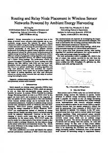
5 Number of nodes = 10

120 100

1

2

3

4

5

6

7

8

100

Y coordinate (m)

Y coordinate (m)

1

2

3

4

5

6

7

8

9

10

11

12

13

14

15

16

80

80 60 40 20

9

10

11

12

13

14

15

16

60 40 20

0 −20 −20

Number of nodes = 13

120

0

0

20

40 60 X coordinate (m)

80

100

−20 −20

120

0

20

40

60

80

100

120

X coordinate (m)

(a) 10 sensor nodes

(b) 13 sensor nodes Number of nodes = 16

120 100

1

2

3

4

5

6

7

8

9

10

11

12

13

14

15

16

Y coordinate (m)

80 60 40 20 0 −20 −20

0

20

40

60

80

100

120

X coordinate (m)

(c) 16 sensor nodes

Figure 5: Sensor nodes position.

that TPSMA would be able to offer higher coverage with fewer sensor nodes. This is due to the fact that the objective function of TPSMA proposed in this work is on the maximum coverage ratio while minimax and lexmin are focusing on the distance of the sensor nodes with the monitored locations. Distance will not necessarily give maximum overall coverage.

4.2. Sensor Nodes Positions. Figure 5 illustrates 10, 13, and 16 sensor nodes’ positions, respectively. The red stars show the access points of the monitored locations while the black stars indicate the sensor nodes. The blue circles show the coverage of the sensor nodes. Figure 5(a) shows WSN deployed with 10 sensor nodes where it is clearly shown that 5 locations are not covered by any sensors nodes while, with 13 sensor nodes, all locations are fully covered as illustrated in Figure 5(b). As predicted, as shown in Figure 5(c), all surveillance locations are completely covered when WSN is deployed with 16 sensor

nodes because all locations are equipped with a sensor node. Based on this result, it can be concluded that our WSN model needs only 13 sensor nodes in order to cover 16 monitored locations when it is deployed with the TPSMA. Hence, the deployment cost will be reduced around 20%.

4.3. Network Uniformity. Uniformity is used to estimate the system lifetime where WSN lifetime can be defined as the shortest lifetime of all sensor nodes [9]. This is due to the fact that uniformly distributed sensor nodes spend energy more evenly through the network [22]. Furthermore, fewer nodes are required to cover the monitored region if the sensor nodes are evenly distributed. WSN with smaller uniformity is considered more evenly distributed in the monitoring area. The mean distances for all nodes to their neighbouring nodes in a uniformly distributed network are almost equal, and hence the expected energy consumption per communication

6


5. Conclusions and Future Work

Uniformity versus number of sensor nodes 1.2

A sensor node placement scheme based on TPSMA has been proposed in order to ensure that the WSN coverage will be maximized for effective monitoring. The network model presented in this paper is an area that consists of several equal widths monitored locations. Based on the simulation results obtained, it can be concluded that WSN deployed with maximum coverage TPSMA sensor nodes placement scheme offers considerably higher coverage ratio and lower uniformity value compared to minimax and lexmin schemes. This result implies that WSN deployed with proposed scheme is expected to provide higher coverage with longer lifetimes. Further work would focus on developing a multiobjective TPSMA sensor node placement scheme.

1

Uniformity

0.8 0.6 0.4 0.2 0 10

11

12 13 14 Number of sensor nodes

15

16

References

TPSMA Minimax Lexmin

Figure 6: Uniformity versus number of sensor nodes.

as well as the expected lifetime of each node is almost equal. Thus, full energy utilization at each node and longer system lifetime of the network are expected. Uniformity can be determined by computing the local uniformity at each sensor node using (8) followed by the network uniformity by using (9) [22]. Only neighbouring nodes that are located within its communication range are considered for local uniformity 𝑈𝑖 = √ (

𝐾

2 1 𝑖 ∑ (𝐷 − 𝑀𝑖 ) ), 𝐾𝑖 𝑗=1 𝑖,𝑗

(8)

where 𝐾𝑖 is the total number of neighbouring nodes, 𝐷𝑖,𝑗 is the distance between ith and jth nodes, and 𝑀𝑖 represents the mean distance between ith node and its neighbours 𝑈=

1 𝑁 ∑𝑈, 𝑁 𝑖=1 𝑖

(9)

where N represents the total number of sensor nodes. Figure 6 exhibits the uniformity value of WSN for different numbers of sensor nodes. As can be seen, the uniformity value decreases as the number of sensor nodes increases because uniformity metric is determined by the communication range and density of sensor nodes [9]. This indicates that WSN with higher sensor nodes will have longer lifetime. As compared to minimax and lexmin schemes, TPSMA gives lower uniformity. Uniformity given by TPSMA is nearly 80% lower than uniformity given by minimax when the WSN is deployed with 10 sensor nodes and approximately around 15% when it is using lexmin technique. From this observation, it can be said that sensor node placement with the proposed TPSMA scheme is expected to provide longer lifetime compared to the other two schemes.

[1] F. Oldewurtel and P. Mähönen, “Analysis of enhanced deployment models for sensor networks,” in Proceedings of the 71st IEEE Vehicular Technology Conference (VTC 2010-Spring), pp. 1–5, Taipei, Taiwan, May 2010. [2] M. Romoozi, M. Vahidipour, M. Romoozi, and S. Maghsoodi, “Genetic algorithm for energy efficient & coverage-preserved positioning in wireless sensor networks,” in Proceedings of the International Conference on Intelligent Computing and Cognitive Informatics (ICICCI ’10), pp. 22–25, Kuala Lumpur, Malaysia, June 2010. [3] M. R. Ingle and N. Bawane, “An energy efficient deployment of nodes in wireless sensor network using Voronoi diagram,” in Proceedings of the 3rd International Conference on Electronics Computer Technology (ICECT ’11), pp. 307–311, Kanyakumari, India, April 2011. [4] L. C. Shiu, C. Y. Lee, and C. S. Yang, “The divide-and-conquer deployment algorithm based on triangles for wireless sensor networks,” IEEE Sensors Journal, vol. 11, no. 3, pp. 781–790, 2011. [5] S. C. Huang, “Energy-aware, self-deploying approaches for wireless sensor networks,” in Proceedings of the 24th IEEE International Conference on Advanced Information Networking and Applications (AINA ’10), pp. 896–901, Perth, Australia, April 2010. [6] S. M. A. Salehizadeh, A. Dirafzoon, M. B. Menhaj, and A. Afshar, “Coverage in wireless sensor networks based on individual particle optimization,” in Proceedings of the International Conference on Networking, Sensing and Control (ICNSC ’10), pp. 501–506, Chicago, Ill, USA, April 2010. [7] D. Zorbas and T. Razafindralambo, “Wireless sensor network redeployment under the target coverage constraint,” in Proceedings of the 5th International Conference on New Technologies, Mobility and Security (NTMS ’12), pp. 1–5, Istanbul, Turkey, May 2012. [8] H. M. Ammari, “On the problem of k-coverage in missionoriented mobile wireless sensor networks,” Computer Networks, vol. 56, no. 7, pp. 1935–1950, 2012. [9] X. Wang and S. Wang, “Hierarchical deployment optimization for wireless sensor networks,” IEEE Transactions on Mobile Computing, vol. 10, no. 7, pp. 1028–1041, 2011. [10] L. Zhiming and L. Lin, “Sensor node deployment in wireless sensor networks based on improved particle swarm optimization,” in Proceedings of the International Conference on Applied


[11]

[12]

[13]

[14]

[15]

[16]

[17]

[18]

[19]

[20]

[21]

[22]

Superconductivity and Electromagnetic Devices (ASEMD ’09), pp. 215–217, Chengdu, China, September 2009. K. S. S. Rani and N. Devarajan, “Optimization model for sensor node deployment,” European Journal of Scientific Research, vol. 70, no. 4, pp. 491–498, 2012. J. Zhao and H. Sun, “Intelligent single particle optimizer based wireless sensor networks adaptive coverage,” Journal of Convergence Information Technology, vol. 7, no. 2, pp. 153–159, 2012. N. A. B. A. Aziz, A. W. Mohemmed, and M. Y. Alias, “A wireless sensor network coverage optimization algorithm based on particle swarm optimization and voronoi diagram,” in Proceedings of the IEEE International Conference on Networking, Sensing and Control (ICNSC ’09), pp. 602–607, Okayama, Japan, March 2009. N. A. B. A. Aziz, A. W. Mohemmed, and B. S. D. Sagar, “Particle swarm optimization and Voronoi diagram for wireless sensor networks coverage optimization,” in Proceedings of the International Conference on Intelligent and Advanced Systems (ICIAS ’07), pp. 961–965, Kuala Lumpur, Malaysia, November 2007. W. Yiyue, L. Hongmei, and H. Hengyang, “Wireless sensor network deployment using an optimized artificial fish swarm algorithm,” in Proceedings of the International Conference on Computer Science and Electronics Engineering (ICCSEE ’12), vol. 2, pp. 90–94, Hangzhou, China, March 2012. L. Zhang, D. Li, H. Zhu, and L. Cui, “OPEN: an optimisation scheme of N-node coverage in wireless sensor networks,” IET Wireless Sensor Systems, vol. 2, no. 1, pp. 40–51, 2012. C. M. Begg, K. S. Begg, J. T. Du Toit, and M. G. L. Mills, “Scentmarking behaviour of the honey badger, Mellivora capensis (Mustelidae), in the Southern Kalahari,” Animal Behaviour, vol. 66, no. 5, pp. 917–929, 2003. K. A. Descovich, A. T. Lisle, S. Johnston, V. Nicolson, and C. J. C. Phillips, “Differential responses of captive southern hairy-nosed wombats (Lasiorhinus latifrons) to the presence of faeces from different species and male and female conspecifics,” Applied Animal Behaviour Science, vol. 138, no. 1, pp. 110–117, 2012. R. Kershner, “The number of circles covering a set,” The American Journal of Mathematics, vol. 61, no. 3, pp. 665–671, 1939. H. Z. Abidin and N. M. Din, “Sensor node placement based on minimax for effective surveillance,” in Proceedings of the IEEE Symposium on Industrial Electronics and Applications (ISIEA ’12), pp. 7–11, Bandung, Indonesia, September 2012. H. Z. Abidin and N. M. Din, “Sensor node placement based on lexicographic minimax,” in Proceedings of the International Symposium on Telecommunication Technologies (ISTT ’12), pp. 82–87, Kuala Lumpur, Malaysia, November 2012. Y. Zhang and L. Wang, “A distributed sensor deployment algorithm of mobile sensor network,” in Proceedings of the 8th World Congress on Intelligent Control and Automation (WCICA ’10), pp. 6963–6968, Jinan, China, July 2010.

7

International Journal of

Rotating Machinery

Engineering Journal of

Hindawi Publishing Corporation http://www.hindawi.com

Volume 2014

The Scientific World Journal Hindawi Publishing Corporation http://www.hindawi.com

Volume 2014


Distributed Sensor Networks

Journal of

Sensors Hindawi Publishing Corporation http://www.hindawi.com

Volume 2014


Volume 2014


Volume 2014

Journal of

Control Science and Engineering

Advances in

Civil Engineering Hindawi Publishing Corporation http://www.hindawi.com


Volume 2014

Volume 2014

Submit your manuscripts at http://www.hindawi.com Journal of

Journal of

Electrical and Computer Engineering

Robotics Hindawi Publishing Corporation http://www.hindawi.com


Volume 2014

Volume 2014

VLSI Design Advances in OptoElectronics


Navigation and Observation Hindawi Publishing Corporation http://www.hindawi.com

Volume 2014



Chemical Engineering Hindawi Publishing Corporation http://www.hindawi.com

Volume 2014

Volume 2014

Active and Passive Electronic Components

Antennas and Propagation Hindawi Publishing Corporation http://www.hindawi.com

Aerospace Engineering


Volume 2014


Volume 2014

Volume 2014




Modelling & Simulation in Engineering

Volume 2014


Volume 2014

Shock and Vibration Hindawi Publishing Corporation http://www.hindawi.com

Volume 2014

Advances in

Acoustics and Vibration Hindawi Publishing Corporation http://www.hindawi.com

Volume 2014