Jacobian Code Generated by Source Transformation and ... - CiteSeerX

Jacobian Code Generated by Source Transformation and Vertex Elimination can be as Efficient as Hand-Coding SHAUN A. FORTH, MOHAMED TADJOUDDINE and JOHN D. PRYCE Cranfield University (Shrivenham Campus) and JOHN K. REID JKR Associates This paper presents the first extended set of results from EliAD, a source-transformation implementation of the vertex-elimination Automatic Differentiation approach to calculating the Jacobians of functions defined by Fortran code (Griewank and Reese, Automatic Differentiation of Algorithms: Theory, Implementation, and Application, 1991, pp. 126-135). We introduce the necessary theory in terms of well known algorithms of numerical linear algebra applied to the linear, extended Jacobian system that prescribes the relationship between the derivatives of all variables in the function code. Using an example, we highlight the potential for numerical instability in vertex-elimination. We describe the source transformation implementation of our tool EliAD and present results from 5 test cases, 4 of which are taken from the MINPACK-2 collection (Averick et al, Report ANL/MCS-TM-150, 1992) and for which hand-coded Jacobian codes are available. On 5 computer/compiler platforms, we show that the Jacobian code obtained by EliAD is as efficient as hand-coded Jacobian code. It is also between 2 to 20 times more efficient than that produced by current, state of the art, Automatic Differentiation tools even when such tools make use of sophisticated techniques such as sparse Jacobian compression. We demonstrate the effectiveness of reverse-ordered pre-elimination from the (successively updated) extended Jacobian system of all intermediate variables used once. Thereafter, the monotonic forward/reverse ordered eliminations of all other intermediates is shown to be very efficient. On only one test case were orderings determined by the Markowitz or related VLR heuristics found superior. A re-ordering of the statements of the Jacobian code, with the aim of reducing reads and writes of data from cache to registers, was found to have mixed effects but could be very beneficial. Categories and Subject Descriptors: G.1.0 [General]: Stability (and instability); G.1.4 [Quadrature and Numerical Differentiation]: Automatic differentiation; G.1.5 [Roots of Nonlinear Equations]: Systems of equations; G.1.6 [Optimization]: Least squares methods; G.4 [Mathematical Software]: Efficiency General Terms: Algorithms, Performance Additional Key Words and Phrases: Jacobians, source transformation, vertex elimination

c

ACM, (2004). This is the author’s version of the work. It is posted here by permission of ACM for your personal use. Not for redistribution. The definitive version was published in ACM Transactions on Mathematical Software , VOL 30, ISSN:0098-3500, (September 2004) http://doi.acm.org/10.1145/1024074.1024076 Work funded by the UK’s EPSRC and MOD under grant GR/R21882. Author’s addresses: S.A. Forth, M. Tadjouddine (Engineering Systems Department) & J.D. Pryce (Communications and Information Sytems Engineering), Cranfield University (Shrivenham Campus), Shrivenham, Swindon SN6 8LA, UK; J.K. Reid, JKR Associates and Rutherford Appleton Laboratory, Atlas Centre, Rutherford Appleton Laboratory, Didcot, Oxon OX11 OQX, UK. Permission to make digital/hard copy of all or part of this material without fee for personal or classroom use provided that the copies are not made or distributed for profit or commercial advantage, the ACM copyright/server notice, the title of the publication, and its date appear, and notice is given that copying is by permission of the ACM, Inc. To copy otherwise, to republish, to post on servers, or to redistribute to lists requires prior specific permission and/or a fee. c 2004 ACM 0098-3500/2004/1200-0266 $5.00

ACM Transactions on Mathematical Software, Vol. 30, No. 3, Sep. 2004, Pages 266–299.

October 11, 2004

Jacobian Code by Vertex Elimination

GLOSSARY A Adjoint matrix ci,j Local derivative ∂Φi /∂uj C Matrix of local derivatives D Solution of extended Jacobian system ei i-th column of unit matrix f Given function ∇f (x) Jacobian matrix, of order m × n m Number of dependent variables n Number of independent variables N =n+p+m N|c|=1 Number of unit entries ci,j = ±1 in C N|c|6=1 Number of non-unit entries in C Nevals Number of separate evaluations timed Nrepet Number of repeats of timing test

p P q Q S si ui u v wi w W x y

·

267

Number of intermediate variables Matrix associated with extended system Number of columns in S Matrix associated with extended system Seed matrix of order n × q or m × q i-th column of S i-th code variable All active variables Variables of the code-list i-th intermediate variable Intermediate variables Computational work Independent variables Dependent variables

1. INTRODUCTION Automatic Differentiation (AD) concerns the process of taking a function y = f (x), with f defined by a computer code, that maps independent variables x ∈ IR n to dependent variables y ∈ IRm and then constructing new code that will also calculate derivatives of f . AD relies on the fact that each statement of the code involving floating-point numbers may be individually differentiated. The forward mode of AD creates new code that, for each of the code’s variables, calculates the numerical values of the variable and its derivatives with respect to the independent variables. Reverse (or adjoint) mode AD produces code that passes forward through the original code storing information required for a reverse pass in which the sensitivities of the nominated dependent variables to changes in the values of the code’s variables are calculated. A thorough introduction to the field may be found in [Griewank 2000] and further theoretical results and applications may be found in the collections [Griewank and Corliss 1991; Berz et al. 1996; Corliss et al. 2001]. AD software tools exist for codes written in Fortran [Bischof et al. 1996; Giering and Kaminski 1998; Faure and Papegay 1998; Pryce and Reid 1998], C and C++ [Bischof et al. 1997; Bendtsen and Stauning 1996; Griewank et al. 1996] and Matlab [Verma 1998; Forth 2001; Bischof et al. 2002] amongst other programming languages. These tools implement AD in one of two ways, source transformation or operator overloading. Source transformation [Griewank 2000, Section 5.7-5.8] involves use of sophisticated compiler techniques. For the forward mode, new code is produced that, when executed, calculates derivatives as well as values for the dependent variables. In reverse mode, new code is produced that will calculate so-called adjoint values backwards through an enhanced version of the original code in such a way as to calculate ST ∇f (x) for any matrix S with m rows. Alternatively, the operator overloading approach [Griewank 2000, Section 5.1-5.6] utilises a feature available in some modern, object-oriented computer languages. New types of variable are defined that store the variable’s value and, for forward mode, also store its derivatives. For reverse mode, instead of derivatives, sufficient information is saved (to a so-called tape) to enable the required reverse propagation of sensitivities. In both cases, arithmetic operations and intrinsic functions are ACM Transactions on Mathematical Software, Vol. 30, No. 3, Sep. 2004.

268

·

Shaun A. Forth et al.

March 8th 2004

extended to the new types. For languages such as Fortran or C (for which optimising compilers exist) and applied to code featuring scalar assignments, it is generally found that the source transformation approach produces more efficient derivative code (see for example [Tadjouddine et al. 2001; Pryce and Reid 1998]). Our work is motivated by the particular requirement for Jacobian code in solving systems of nonlinear equations via Newton’s, or a related method. Such systems arise in applications such as computational fluid dynamics, computational chemistry, and data-fitting. For examples, see the test cases of [Averick et al. 1992] and references therein. In such cases, the system Jacobian may be needed for direct solution of a Newton update. Alternatively, when using Krylov-based solvers for which Jacobian-vector products may be evaluated by finite differencing or conventional AD tools, the Jacobian frequently needs to be determined for preconditioning, for example, when using incomplete LU factorisation [Hovland and McInnes 2001]. When discussing sparsity, we will use the term entry for a matrix coefficient that we represent explicitly because we cannot be sure that it is zero. An entry may ‘accidentally’ have the value zero, so the term ‘nonzero’ is not suitable. The structure of the rest of this paper is as follows. In Section 2 and Section 3, we review the matrix interpretation of the conventional forward and reverse modes of AD and then the vertex elimination approach of [Griewank and Reese 1991]. This is necessary to understand the implementation of our vertex elimination tool EliAD. EliAD is implemented via source transformation as described in Section 4. Our test environment is explained in Section 5. In Section 6, we present and discuss an extended set of results from EliAD. For these test cases, we demonstrate that AD via vertex elimination and source transformation enables the calculation of Jacobians as fast as hand-coded Jacobian code and with more than twice the efficiency of present AD tools and techniques. Section 7 presents conclusions and the outlook for extending EliAD’s coverage of Fortran and improving it to produce even faster Jacobian code. 2. MATRIX INTERPRETATION OF AUTOMATIC DIFFERENTIATION The matrix interpretation of AD [Griewank 2000, Section 8.1] allows us to view the standard forward and reverse modes of AD in terms of the well-known forward and back substitution algorithms for systems of linear equations with triangular coefficient matrices. In Section 2.1, we introduce the lower triangular extended Jacobian system and in Section 2.2 we indicate how this system is solved in forward and reverse mode AD. We then consider the exploitation of sparsity, the number of floating-point operations involved, and how to treat the temporary variables that occur within statements. 2.1 The Extended Jacobian System For a function f : x ∈ IRn 7→ y ∈ IRm that is defined by computer code and which we wish to differentiate, we define three (sub)groups of the code’s variables: independent variables: x = (xi , i = 1, . . . , n) whose values must be supplied and with respect to which the derivatives ∂y/∂x are required, dependent variables: y = (yi , i = 1, . . . , m) which must be calculated and whose ACM Transactions on Mathematical Software, Vol. 30, No. 3, Sep. 2004.

October 11, 2004


·

269

derivatives are required, intermediate variables: w = (wi , i = 1, . . . , p) whose values are calculated (perhaps indirectly) from the x and which are needed to calculate (perhaps indirectly) the y. Collectively, these variables are termed active variables. We define inactive variables as those which are not active. Example 2.1 Example Code. For the code fragment w1 w2 w3 y1 y2

= log(x1 ∗ x2 ) = x2 ∗ x23 − a = b ∗ w1 + x2 /x3 = w12 + w2 − x2 √ = w3 − w 2

we wish to calculate ∂(y1 , y2 )/∂(x1 , x2 , x3 ). Hence x1 , x2 , x3 are the n=3 independent variables, y1 , y2 are the m=2 dependent variables, and w1 , w2 , w3 are the p=3 intermediate variables. Values of the variables a, b must be supplied but, since we do not require derivatives with respect to them, they are inactive. For the purposes of analysis, we regard an execution of the function code as defining N = n + p + m internal variables ui , i = 1, . . . , N in the following manner. First there are n copies of the independent variables to the internal variables, ui = xi , i = 1, . . . n,

(1)

followed by the p + m statements of the code ui = Φi ({uj }j≺i ), i = n + 1, . . . , N,

(2)

where the precedence relation j ≺ i means that the variable uj is involved in the expression Φi . Each Φi represents a composition of one or more elemental/intrinsic functions or elemental/intrinsic operators of the programming language. For the most part, we will assume that no expression for a dependent variable involves another dependent variable, that is, if i > n + p and j ≺ i, then j ≤ n + p. This may be ensured by making a copy of any dependent variable used to calculate another dependent variable, but we will also explain how to avoid the need for this. Example 2.2 Example Code. The code fragment of Example 2.1 may be rewritten in the form of (1) to (2) as  u1 = x 1     u2 = x 2     u3 = x 3    u4 = Φ4 (u1 , u2 ) = log(u1 ∗ u2 ) . u5 = Φ5 (u2 , u3 ) = u2 ∗ u23 − a    u6 = Φ6 (u2 , u3 , u4 ) = b ∗ u4 + u2 /u3     u7 = Φ7 (u2 , u4 , u5 ) = u24 + u5 − u2    √  u8 = Φ8 (u5 , u6 ) = u6 − u 5 ACM Transactions on Mathematical Software, Vol. 30, No. 3, Sep. 2004.

270

·


March 8th 2004

The assignments of (1) and (2) can be written as the following system of nonlinear equations 0 = x i − ui , i = 1, . . . , n . (3) 0 = Φi ({uj }j≺i ) − ui ), i = n + 1, . . . , N We assume that the functions Φi have continuous first derivatives, define the gradient operator ∇ by ∇ = (∂/∂x1 , . . . , ∂/∂xn ), and differentiate (3) with respect to the independent variables x1 , . . . , xn , to give −∇ui = −ei , i = 1, . . . , n P , (4) i = n + 1, . . . , N j≺i ci,j ∇uj − ∇ui = 0,

where ei is the n-vector with unit entry in position i and ci,j are the local derivatives ci,j = ∂Φi /∂uj . On defining the matrix C = {ci,j }1≤i,j≤N to be composed of all such entries and zeros elsewhere, the linear system (4) can be compactly rewritten as the extended Jacobian system (C − IN )D = −P, with D = ∇u and P=

In 0(m+p)×n

.

(5)

(6)

The matrix C−IN is called the extended Jacobian and is necessarily lower triangular because each value ui is calculated from previously calculated values uj with j ≺ i. We define N|c|=1 to be the number of entries in C taking the value ±1 and N|c|6=1 to be the number of other entries. Example 2.3 Extended Jacobian System. For our example code, the extended Jacobian system is given by      −1 ∇u1 −1 0 0    ∇u2   0 −1 0  −1         ∇u3   0 0 −1  −1       c4,1 c4,2   ∇u4   0 0 0  −1   =     ∇u5   0 0 0  , c5,2 c5,3 −1         ∇u6   0 0 0  c6,2 c6,3 c6,4 −1         ∇u7   0 0 0  c7,2 c7,4 c7,5 −1 ∇u8 0 0 0 c8,5 c8,6 −1 with entries in the extended Jacobian given by c4,1 c4,2 c5,2 c5,3 c6,2 c6,3

= 1/u1 , = 1/u2 , = u23 , = 2 ∗ u 2 ∗ u3 , = 1/u3 , = −u2 /u23 ,

We see that N|c|=1 = 3 and N|c|6=1 = 9.

c6,4 c7,2 c7,4 c7,5 c8,5 c8,6

 =b     = −1,    = 2 ∗ u4 , . = 1,     = −1   √  = 1/(2 u6 )

ACM Transactions on Mathematical Software, Vol. 30, No. 3, Sep. 2004.

(7)

October 11, 2004


·

271

2.2 Forward and Reverse Mode AD In the forward method, we solve the lower triangular system (5) for the n columns of D by forward substitution, then extract the last m rows to obtain the Jacobian. By defining the matrix Q to be 0(n+p)×m , (8) Q= Im we can express the solution of equation (5) and the extraction of the final m rows of D as ∇f = QT (C − IN )−1 (−P).

(9)

(C − IN )T A = −Q,

(10)

If we group the terms as ∇f = QT [(C − IN )−1 (−P)], we have a formal deof forward mode AD. Alternatively, by grouping equation (9) as ∇f = scription (−QT )(C − IN )−1 P, and defining adjoint quantities A as the solution, by backsubstitution, of the upper-triangular system, T

we obtain the Jacobian as the first n columns of A , or more formally ∇f = AT P. This is a matrix interpretation of reverse mode AD [Griewank 2000, p. 161–162]. It should be noted that present AD tools, such as Tamc, are designed to calculate an arbitrary Jacobian-matrix product (forward mode) or an arbitrary matrixJacobian product (reverse mode). Consequently, they allow for P to be of the form S for an arbitrary full matrix S with n rows and q columns and Q P= 0(m+p)×q 0(n+p)×q to be of the form Q = for an arbitrary full matrix S with m rows and S q columns. Such a matrix S is termed a seed matrix. We denote its i-th column by si . Of course, the solutions D of (5) or A of (10) are then no longer simple derivatives or adjoints, but are linear combinations ∇f si of derivatives or sTj ∇f of adjoints. It may readily be verified that if S is full, the solution of (5) or (10) is full (apart from ‘accidental’ cancellations where two values sum to zero) since each of the last p+m rows and each of the first n+p columns of C has at least one entry. To calculate the Jacobian ∇f using such tools, the seed matrix S must be set to In (forward mode) or Im (reverse mode). Let us consider these two approaches for our Example 2.3. Example 2.4 Forward mode AD. Forward mode AD solves the linear system of Example 2.3 using 9×3 = 27 multiplications and 7×3 = 21 additions/subtractions, that is, 48 floating-point operations (flops). Example 2.5 Reverse/Adjoint Mode AD. For Example 2.3 the adjoint system is solved using 9×2 = 18 multiplications and 5×2 = 10 additions/subtractions, that is, 28 flops. For our simple example, reverse mode AD uses fewer arithmetic operations than forward mode. In both examples, we have neglected multiplications by unit entries ci,j = ±1. We have, however, counted the multiplications and additions by zero that occur when S is not full. This is because the basic operation is the addition of a multiple of ∇ui to ∇uj and testing for zeros in ∇ui would slow the code. ACM Transactions on Mathematical Software, Vol. 30, No. 3, Sep. 2004.

272

·


March 8th 2004

2.3 Taking Account of Sparsity If no account is taken of sparsity in S and if the given function f takes time W (f ), forward mode AD calculates the Jacobian in time O(n) × W (f ) and reverse mode does so in time O(m)×W (f ) [Griewank 2000]. For problems with many independent variables (n 1) and few dependents, we see that reverse mode is to be preferred (e.g. large scale optimization). For Jacobians with known sparsity pattern, there are established techniques for reducing the size of the seed matrix S needed to calculate all nonzero entries of ∇f (x) [Griewank 2000, Chap. 7]. Such techniques, collectively termed Jacobian compression, frequently reduce the size, but not to less than q columns in forward mode or q rows in reverse with q the maximum number of entries in any row (forward mode) or column (reverse mode) of the Jacobian. Another possibility is to employ a data structure that permits all operations with values that are known to be zero to be avoided completely. This is the approach taken by our code EliAD. Explicit code is generated for each of the elimination operations ci,j = ci,j − ci,k ck,j for which ci,k and ck,j are both entries. No code is generated where is it known a priori that either ci,k or ck,j is always zero. The techniques discussed so far in this section assume that the sparsity structure is fixed, so that the set of vectors or generated code needs to be determined once, and they are thus static exploitations of the Jacobian sparsity. An alternative is via the dynamic exploitation of sparsity. Here, the data are stored in some sparse format that is adjusted dynamically (at run time). Prime examples of such an approach are the use of the SparsLinC library in Adifor [Bischof et al. 1996; Bischof et al. 1996], use of sparse options in AD01 [Pryce and Reid 1998], and exploitation of the sparse matrix class of Matlab [Coleman and Verma 1998; Forth 2001]. The formal operations count for such an approach is low, but the overhead of manipulating the sparse storage typically makes them uncompetitive unless the sparsity structure is not fixed [Griewank 2000, p. 156]. The approach is also of use in determining a fixed sparsity structure prior to Jacobian compression. 2.4 Computational Cost of Forward and Reverse Mode AD For a given function f , we assume the computational cost W (∇f ) of evaluating its derivatives via AD may be written as W (∇f ) = W (f ) + W (C) + W (linear solve),

(11)

where: — W (f ) is the cost of evaluating the original function. — W (C) is the cost of evaluating C, that is, all the local derivatives ci,j . — W (linear solve) is the cost of solving the linear system (5) or (10). We will measure the cost in floating-point operations (flops), concentrating on W (linear solve) since we can have little influence on the other two costs. ACM Transactions on Mathematical Software, Vol. 30, No. 3, Sep. 2004.

October 11, 2004


·

273

[Griewank 2000, Chap. 3] takes account of the time required for data transfers from and to the floating-point registers under rather conservative conditions. However, as we shall see in Sections 3.1 and 4, our optimized derivative code may access extended Jacobian entries in a non-sequential way and this, together with the effects of compiler optimizations make this time difficult to quantify and so, regretfully, we neglect it in this subsection. This approximation is in line with that of previous work [Griewank and Reese 1991], [Griewank 2000, Chap. 8]. For forward mode AD and without exploiting Jacobian compression or dynamic sparsity (see Section 2.3), the cost of the linear solve of (5) is given by W (linear solve (forward mode)) = n(2N|c|6=1 + N|c|=1 − p − m).

(12)

We incur n multiplications when multiplying a row by a ci,j 6= ±1 and n additions for all entries as we accumulate the vectors to the ui . We subtract the cost of n(m + p) additions since the first gradient in each line of the forward substitution is assigned and not added to the intermediate’s or dependent’s derivatives. For a sparse Jacobian, (forward) Jacobian compression techniques frequently allow the Jacobian ∇f (x) to be recovered from q < n Jacobian-vector products ∇f (x)si , i = 1, . . . , q. Clearly, the cost of calculating this is given by (12), but with n replaced by q. Similarly, for reverse mode AD, the computational cost of the linear solve associated with (10) is W (linear solve (reverse mode)) = m(2N|c|6=1 + N|c|=1 − p − n).

(13) s Tj ∇f (x),

If Jacobian compression is possible, we propagate q vector-Jacobian products j = 1, . . . , q, and extract the Jacobian with a resulting cost for the linear solve given by (13) with m replaced by q. 2.5 Statement-Level versus Code-List Differentiation

So far in this paper, we have differentiated each statement locally with respect to the active variables that appear in its right-hand side. This is termed a statementlevel differentiation. An alternative, used later in this paper, is based on the code list [Griewank 2000], in which the original program is rewritten so that the righthand side of each statement has a single unary or binary operation. Example 2.6 Code-List. A possible code list for Example 2.1 is: v1 v2 v3 v4 v5 v6 v7 v8

≡ x1 ≡ x2 ≡ x3 = v1 ∗ v2 = log(v4 ) = v32 = v6 ∗ v2 = v7 − a

v9 = 1/v3 v10 = v2 ∗ v9 v11 = b ∗ v5 v12 = v11 + v10 v13 = v8 − v2 v14 = v52 √ v15 = v12 v16 = v14 + v13 v17 = v15 − v8

(14)

in which the division has been replaced by the nonlinear reciprocal operation followed by a multiplication, and statements are ordered such that the final two variables v16 , v17 correspond to the dependent variables y1 , y2 . ACM Transactions on Mathematical Software, Vol. 30, No. 3, Sep. 2004.

274

·


March 8th 2004

3. AUTOMATIC DIFFERENTIATION BY VERTEX ELIMINATION If there are no intermediate variables (p=0), the second line of equation (4) shows that the matrix C is the Jacobian ∇f (x). [Griewank and Reese 1991] therefore systematically reduced the extended Jacobian system (5) by Gaussian elimination of the intermediate variables to obtain the Jacobian. Their original analysis actually used the computational graph but was later reinterpreted [Griewank 2000] using the extended Jacobian. We defer the graph interpretation until Section 3.2, first introducing vertex elimination via the extended Jacobian description in Section 3.1 since we believe it is more accessible to the scientific computing community. We discuss the connection to standard AD algorithms in Section 3.3. In Section 3.4, we discuss techniques to determine the order in which we choose to eliminate intermediates from the extended Jacobian. In Section 3.5, we show that a poor choice of ordering may lead to accumulation of roundoff and instability. Section 3.6 describes techniques for statement-level differentiation of the function, which motivate the pre-elimination strategy of Section 3.7.

3.1 Reduction of the Extended Jacobian To reduce the extended Jacobian, we apply Gaussian elimination, pivoting on the diagonal entries of the columns corresponding to intermediate variables. In each case, we add multiples of the pivot row to later rows to create zeros below the diagonal in the pivot column. Since the pivot row and pivot column are no longer relevant, we then discard them — this is what makes it Gaussian, rather than the less efficient Jordan, elimination. Note that the form of the extended Jacobian is preserved in the sense that it remains lower triangular with diagonal entries equal to −1. We illustrate this with the extended Jacobian system of Example 2.3. We start with the system



−1

     c4,1      



∇u1   ∇u2 −1    ∇u3 −1    ∇u4 c4,2 −1    ∇u5 c5,2 c5,3 −1    ∇u6 c6,2 c6,3 c6,4 −1    ∇u7 −1 c7,4 1 −1 ∇u8 −1 c8,6 −1





          =          

−1

−1



  −1    .     

(15)

First, pivoting on diagonal 4, we add multiples c6,4 and c7,4 of row 4 to rows 6 and 7. This creates two new entries, or fill-ins, c6,1 = c6,4 ∗ c4,1 , c7,1 = c7,4 ∗ c4,1 , and modifies two entries, c6,2 = c6,2 + c6,4 ∗ c4,2 , c7,2 = −1 + c7,4 ∗ c4,2 . Row and ACM Transactions on Mathematical Software, Vol. 30, No. 3, Sep. 2004.

October 11, 2004


column 4 are now discarded to give      −1 −1 ∇u1    ∇u2    −1 −1         ∇u3    −1 −1         .   c c −1 ∇u = 5,2 5,3 5       c6,1 c6,2 c6,3   ∇u6    −1       c7,1 c7,2   ∇u7    1 −1 ∇u8 −1 c8,6 −1

·

275

(16)

We now pivot on the new diagonal 4. This requires one modification c7,2 = c7,2 + c5,2 and three fill-ins c7,3 = c5,3 , c8,2 = −c5,2 , c8,3 = −c5,3 . The pivot row and column are now discarded. For the final pivot step, we have two modifications c8,2 = c8,2 + c8,6 ∗ c6,2 , c8,3 = c8,3 + c8,6 ∗ c6,3 and one fill-in c8,1 = c8,6 ∗ c6,1 to yield      −1 ∇u1 −1   ∇u2     −1 −1        ∇u3  =  .  −1 −1        ∇u7     c7,1 c7,2 c7,3 −1 ∇u8 c8,1 c8,2 c8,3 −1 Clearly, we now have ∇f (x) =

c7,1 c7,2 c7,3 c8,1 c8,2 c8,3

and, neglecting the cost of sign changes, the Jacobian has been calculated with a total cost of 12 floating-point operations (flops). This is a substantial saving over the forward mode of Example 2.4 (48 flops) and reverse mode of Example 2.5 (28 flops). It is trivial to allow for entries ci,j in the final m columns of C (when some expressions for dependent variables involve other dependent variables). We simply perform Gaussian elimination on each such column, but do not discard the pivot row. 3.2 The Computational Graph Description The description of Section 3.1 suggests that Gaussian elimination, rather than vertex elimination, would be a more appropriate name for the algorithms of this paper. To explain the origins of the term vertex elimination we return to the original graph based description of [Griewank and Reese 1991]. In Figure 1(a), we show the computational graph for our example before any eliminations have been performed. The graph has vertices labelled 1 to 8 corresponding to the internal variables u1 to u8 of Example 2.2. Vertices 1 to 3, corresponding to the independent variables, are placed at the bottom of the graph and the dependents, labelled 7 and 8, are at the top. Vertices 4 to 6, corresponding to intermediates, lie in the centre. There is a directed edge from vertex j to vertex i if j ≺ i and the edge is labelled with the associated local derivative ci,j as given in (7). This labelling is what makes it the “linearized” computational graph. The derivative of any dependent variable i with respect to any independent j is ACM Transactions on Mathematical Software, Vol. 30, No. 3, Sep. 2004.

276

·


u7 u8 @ c8,6 I AA OCK @ c7,4 C Ac7,5 c8,5 @u6 : C A

6

c6,4C A 5 c6,2

u 4 C Au c7,2C

I @ 6 I @ @

@ c4,2 C 6 c6,3 @

c5,3 C c5,2 @ c4,1 @ C

@ @ C

@ @C

@u3 u1 u2 a) Original computational graph

u7 u8 @ c8,6 S OCI OCo @ C @u C S c8,3C > 6 C S

6

C C S S C

C c7,1 S C C C S c7,3 C c6,3 C c8,2 S C c C

6,1 c6,2 S C c 7,2 SC C

1

2 SCu3 Cu u c) After elimination of vertex 5 Fig. 1.

March 8th 2004

u7 u8 @ c8,6 I AA OCK @ CA @u6 C Ac7,5 c8,5 >

6 C A

C

c 6,2 u A c7,1 5 C

6 I @ C@

c6,3 c C c5,2 @

c5,3 6,1

@ c7,2C C

@ u 1 Cu @u3

2 b) After elimination of vertex 4

u7 u8 7 OC S OCo C C S C S C S C C C c8,3 C S c7,1 C S C Sc7,3 C c8,1 C S C C S C c7,2C c8,2 SC C SCu3 2 Cu 1 u d) After elimination of vertex 6

Graph representation of the vertex elimination of Section 3.1

given by the sum of the products of all edge labels for paths connecting j to i in the graph [Griewank 2000, p. 169]. For example, u7 is connected to u2 via three paths given by the 3 sets of edge labels {c7,4 , c4,2 }, {c7,2 } and {c7,5 , c5,2 } and so,

∂u7 = c7,4 ∗ c4,2 + c7,2 + c7,5 ∗ c5,2 . ∂u2 Consequently, we see that a vertex labelled k and all associated edges c k,j≺k , ci,k≺i (short for any ck,j where j ≺ k, resp. ci,k where k ≺ i), can be eliminated from the graph by using the following procedure. We take each out-edge labelled ci,k≺i leaving vertex k and each in-edge ck,j≺k entering and add the product ci,k ∗ ck,j to the edge ci,j , creating a new edge ci,j if required. The edges ci,k≺i ,ck,j≺k may now be removed from the graph since their contributions to the Jacobian calculation have been added to other edges of the graph. Example 3.1 Vertex Elimination in the Computational Graph. Vertex 4 in Figure 1(a) has two in-edges c4,1 , c4,2 and two out-edges c7,4 , c6,4 . Consequently, there are four products of out-edges with in-edges c 7,4 ∗c4,1 , c7,4 ∗c4,2 , c6,4 ∗ c4,1 and c6,4 ∗ c4,1 . Of these products, two are added to existing edges of the graph c7,2 = c7,2 + c7,4 ∗ c4,2 , c6,2 = c6,2 + c6,4 ∗ c4,2 , and two require new edges (shown in bold in Figure 1(b)) to be added, c6,1 = c6,4 ∗ c4,1 , c7,1 = c7,4 ∗ c4,1 . Once these operations have been performed, vertex 4 and its associated edges may be removed leaving the graph of Figure 1(b). ACM Transactions on Mathematical Software, Vol. 30, No. 3, Sep. 2004.

October 11, 2004


·

277

Comparison of the operations of Example 3.1 with the first Gaussian elimination performed on the extended Jacobian of Section 3.1 demonstrates the equivalence of the two interpretations, matrix and graph, of vertex elimination. Figures 1(c) and 1(d) show the graph after elimination of vertices 5 and 6 respectively. The numerical operations involved to update edge labels are precisely those of Section 3.1 used to update the extended Jacobian entries. Figure 1(d) shows the graph after eliminating all intermediate vertices and associated edges. We see that the graph is bipartite, i.e. the vertices form two disjoint sets, independent and dependent, and the only edges go from an independent to a dependent. Each edge’s label corresponds to a desired partial derivative. Any entries ci,j in the final m columns of C correspond to edges between dependent variables. Their elimination (see final paragraph of Section 3.1) corresponds to elimination of edges. For our example, if there is an edge c8,7 and it is eliminated last, all the edges to node 8 must be modified: c8,i = c8,i + c7,i ∗ c8,7 , i = 1, 2, 3. 3.3 The Connection to Standard AD Algorithms There is a close relationship between the elimination algorithm with the pivots taken in forward order, and the Forward Mode of AD, equivalent to solving the system (5) by forward substitution (Section 2.2). We may write the extended Jacobian C − I in the equivalent block form [Griewank 2000, p. 22],   −In 0 0 C − I =  B L − Ip 0  , (17) R T −Im

with L strictly lower-triangular. We must now solve,      −In 0 0 ∇x −In  B L − Ip 0   ∇w  =  0  . R T −Im 0 ∇y

(18)

Forward substitution, as for conventional forward mode AD, gives ∇x = In ,

∇w = −(L − Ip )−1 B∇x = −(L − Ip )−1 B, ∇y = R∇x + T∇w = R − T(L − Ip )−1 B. In the elimination approach, we eliminate subdiagonal entries in the L block and all entries in the T block from (18),      −In ∇x −In 0 0  −(L − Ip )−1 B −Ip 0   ∇w  =  0  , (19) 0 ∇y R − T(L − Ip )−1 B 0 −Im

to leave the Jacobian in the lower-left block. The two approaches are thus algebraically equivalent [Griewank 2000, Section 8.1]. We also see that in the forwardsubstitution approach fill-in is confined to the n columns of the system right-hand side matrix, whereas in the elimination approach it is confined to the first n columns of the extended Jacobian. Note that the matrix (L − Ip ) is lower triangular and so the product (L−Ip )−1 B is determined by forward substitution and not by inverting the matrix and multiplying. ACM Transactions on Mathematical Software, Vol. 30, No. 3, Sep. 2004.

278

·


March 8th 2004

Similarly, the Reverse Mode is equivalent to elimination with the pivots taken in reverse order. This confines fill-in to the R and T blocks. It is equivalent to solving the transposed system (10) by back-substitution. For our example, this technique also requires 12 flops to calculate the Jacobian. If full advantage of sparsity is taken, then [Griewank and Reese 1991] showed that the forward and reverse ordered eliminations will never use more floating-point operations than conventional forward and reverse mode AD, even when conventional techniques use features such as Jacobian compression or a sparse representation of gradients and adjoints. 3.4 Elimination Sequences From the above discussion it is clear that, instead of using the elimination approach for calculating Jacobians, we could simply implement forward and reverse mode AD and explicitly account for the sparsity of directional derivatives or adjoints. However, an advantage of the elimination approach is that it removes the restriction to monotonic increasing or decreasing pivot orderings and some other pivot sequence might be chosen. The use of non-monotonic pivot sequences is referred to as crosscountry elimination [Griewank 2000, Chap 8.] and the extra degrees of freedom so gained give scope for reducing the computational cost. However, we do note that the forward and reverse orderings have the advantage of confining fill-in to blocks B and R or R and T. Another pivot ordering is likely to create fill-ins in block L. This block is usually far larger than B, R or T, since there are usually far more intermediate variables than independent or dependent variables. There is therefore a danger of producing a large number of fill-ins which must be removed later in the elimination process and which would compromise efficiency. The problem of choosing a good pivot sequence for Gaussian elimination of sparse matrices has been well studied [Duff et al. 1989]. One of the earliest pivot ordering heuristics is due to [Markowitz 1957]. The Markowitz heuristic involves, at each elimination step, choosing the next pivot to minimize the product of the number of other entries in its row and the number of other entries in its column. This product, known as the Markowitz cost, is an upper bound both on the fill-in at the next elimination step and on the number of multiplications required (noting that pivots are all −1 and that some of the other entries may have the value 1 or −1). Although the Markowitz heuristic is often very successful in reducing the operations count, there are simple examples [Griewank 2000, p. 179] for which it is found to be sub-optimal. In his thesis, [Naumann 1999] suggested the use of what he called the Vertex Lowest Relative (VLR) heuristic also termed Relatively Greedy Markowitz by [Griewank 2000, p. 179]. This VLR heuristic cost is the difference between the current (Markowitz) cost of a candidate pivot and the cost of eliminating it last in the elimination sequence. We have previously noted [Tadjouddine et al. 2001] that the VLR heuristic tends to eliminate those intermediate variables calculated near the start or end of the code after those in the middle. In the event of two or more candidate pivots having an equal minimum Markowitz or VLR cost, then a tie-breaking strategy must be used. [Griewank and Reese 1991] selected the candidate that resulted in most entries in the extended Jacobian being removed. In our work, we choose the last pivot with minimum cost [Tadjouddine et al. 2001]. ACM Transactions on Mathematical Software, Vol. 30, No. 3, Sep. 2004.

October 11, 2004


·

279

3.5 Roundoff The accuracy of automatic differentiation necessarily depends on the accuracy of the calculation of the function and its local derivatives ci,j . If this is ill conditioned, as for example when the “wrong” method for the calculation of a small root of a quadratic equation is employed, the derivative calculation will be ill conditioned too. However, it is important to know if damage might be inflicted by a poor choice of elimination sequence. One of us [Reid 2003] has considered this. The forward method is just forward substitution applied to the system (5) and standard backward error analysis [Wilkinson 1965, pp. 247-248] shows that for each column of P we will have solved a nearby problem (C + δC − IN )d = −p,

(20)

with |δci,j | ≤ (3r/2 + 3)|ci,j |, where r is the largest number of entries in a row of C. Although the perturbations will differ from column to column, we will in each case have done no worse than we would have done for an exact calculation for very slightly perturbed local derivatives ci,j . The same very satisfactory result holds for the backward method since it is back-substitution applied to the system (10). Unfortunately, [Reid 2003] has found an (admittedly artificial) example that shows that another pivot sequence can be unstable. If the entries of C are c2k,2k−1 = 2.0, c2k+1,2k−1 = 2.0, c2k+1,2k = −1.0, k = 1, 2, . . . , l,

(21)

the pivot sequence 1, 3, . . . , 2l − 1, 2, 4, . . . , 2l, leads approximately to the doubling of the size of matrix entries at each stage until 2l − 1. The matrix C − I is not ill-conditioned, so the final solution is not large, but large rounding errors will have occurred in intermediate stages. While this negative result leads us to be cautious, we have not encountered instability in practical cases. 3.6 Statement-Level Differentiation Now consider the statement-level differentiated version of the code, ignoring the possibility of array operations permitted, for example, in the Fortran 95 language. One approach, adopted by Tamc [Giering and Kaminski 1998], is to differentiate each statement symbolically. This has the potential disadvantage of generating local derivative code with many common sub-expressions; though we would expect these to be eliminated by today’s optimising compilers. Alternatively, the right-hand side of a statement may be regarded as composed of the corresponding several lines of the code list, eventually assigning one value to the left-hand side. To obtain the local derivatives ci,j associated with the statement, it is a well established technique to differentiate the local code list using reverse mode AD. This strategy is used by Adifor [Bischof et al. 1998] within an overall forward mode AD approach. 3.7 Reverse Pre-Elimination One way to order the eliminations within the extended Jacobian of the code-list is to follow Adifor by starting with reverse-ordered elimination of the set of intermediate variables within a statement. This may be seen as a sequence of eliminations of intermediate variables with single successors. This is desirable since each such ACM Transactions on Mathematical Software, Vol. 30, No. 3, Sep. 2004.

280

·


March 8th 2004

elimination reduces the number of entries in C by at least one. To see this, suppose the variable has k predecessors and a single successor, consider the square submatrix of order k + 2   C11 − Ik   C21 −1 (22) C31 C32 −1 corresponding to all the variables involved where the variable itself is in the middle. There can be no fill outside this submatrix since there are no entries outside it in the row and column of the intermediate variable. Furthermore, all fill takes place within C31 . Because of our choice of variables, C21 is a full submatrix of order 1×k and C32 is a nonzero 1×1 submatrix. We therefore lose k+1 entries when we discard the pivot row and column and end with k entries in C31 . Thus the number of entries is reduced by at least one (more if C31 starts as nonzero). This suggests that it is desirable to eliminate any intermediate variable with a single successor. We have therefore implemented a reverse pre-elimination strategy in which we repeatedly consider all intermediate variables starting from the last and proceeding to the first and successively eliminate each one encountered which has a single successor. Note that this will include the elimination from the code-list extended Jacobian of all intermediate variables from within any statement and so mimics the statement-level reverse strategy of Adifor [Bischof et al. 1996]. Reverse pre-elimination will also eliminate any variable used in the right-hand side of only one other statement and so reduce the number of arithmetic operations, both in the code-list and the statement-level extended Jacobian. In particular, the result of any unary operation will be eliminated, a process referred to as hoisting in [Bischof 1991]. The elimination AD techniques described above have been implemented in our source transformation AD tool EliAD which we now describe. 4. THE ELIAD TOOL EliAD is a vertex elimination AD tool, written in Java and uses a front-end (parser) and back-end (pretty-printer) generated by ANTLR [Parr et al. 2000]. Though we still regard EliAD as a proof-of-concept tool, it is available from the authors. It uses source-transformation to convert Fortran code for a function f into Fortran code for f and its Jacobian. EliAD performs a bi-directional data flow analysis to determine active variables from user specified independent and dependent variables [Hascoet et al. 2003]. It then performs a symbolic differentiation of each statement of the function (or its code-list) to obtain each subdiagonal entry ci,j of the extended Jacobian. All such entries, and those generated by fill-in during elimination, become separate (scalar) Fortran variables, e.g. c7,1 might appear in the code as the variable c 7 1. Each elimination operation, following a chosen pivot sequence, becomes a set of separate Fortran statements, e.g. the fill-in c7,1 = c7,4 c4,1 becomes c 7 1 = c 7 4*c 4 1 Work is in hand to improve EliAD’s ability to suppress the multiplication if one of the operands is known a priori to be ±1 and perform other such optimizations. ACM Transactions on Mathematical Software, Vol. 30, No. 3, Sep. 2004.

October 11, 2004


·

281

EliAD allows arrays as input arguments provided their indexing is static, that is, can be calculated a priori. In effect, EliAD unrolls them. For instance, if the inputs are two arrays each of length 5, then their elements become input variables x1 to x5 and x6 to x10 , respectively. EliAD allows branching [Tadjouddine et al. 2003], though no such test problems are considered in this paper. Results for one test problem may be found in [Forth and Tadjouddine 2003]. Currently no kind of loop is supported. The chief advantage of this approach is that it permits sparsity in the elimination to be exploited to the maximum. A disadvantage is that the sparsity pattern of the matrix C (or a modest overestimate) must be known a priori. Also, though the generated code runs very fast, its length is roughly proportional to the number of elimination operations, which may be expected to grow more than linearly in the length of the f code. However, as we shall see in Section 6, EliAD has been applied successfully to loop-free subroutines with between 8 to 134 independent, 5 to 252 dependent and over 1000 intermediate variables. After EliAD has built the extended Jacobian, it applies some algorithm — currently an external program — to determine a good pivot sequence using the Markowitz or a related heuristic, and uses this to generate the Jacobian code. 4.1 Generating the Jacobian Code Using the abstract syntax tree of the input code [Aho et al. 1995] and associated symbolic information, EliAD intersperses the original code with assignments that compute local partial derivatives statement by statement. Then, using the given elimination sequence, it generates a series of scalar assignments that eliminate all coefficients of intermediate variables from the extended Jacobian. Each statement computes a new entry or updates an existing entry of the extended Jacobian as may be seen in the following example. Example 4.1 Jacobian Code. The Jacobian code using the reverse ordering — that is, eliminating intermediate variables u6 , u5 and u4 in that order — from the five non-trivial assignments of Example 2.2 could be built up as follows: ! Calculate the values of the variables and local derivatives c_4_1 = 1/u_1; c_4_2 = 1/u_2 u_4 = log(u_1*u_2) c_5_2 = u_3**2; c_5_3 = 2*u_2*u_3 u_5 = u_2*u_3**2-a c_6_2=1/u_3; c_6_3=-u_2/u_3**2; c_6_4=b u_6 = b*u_4+u_2/u_3 c_7_2=-1; c_7_4=2*u_4; c_7_5=1 u_7 = u_4**2+u_5-u_2 c_8_5=-1; c_8_6=1/(2*sqrt(u_6)) u_8 = sqrt(u_6)-u_5 ! Eliminate entries in row 6 c_8_2=c_8_6*c_6_2; c_8_3=c_8_6*c_6_3; c_8_4 = c_8_6*c_6_4 ! Eliminate entries in row 5 c_7_2 = c_7_2+c_7_5*c_5_2; c_7_3=c_7_5*c_5_3 c_8_2=c_8_2+c_8_5*c_5_2; c_8_3=c_8_3+c_8_5*c_5_3 ! Eliminate entries in row 4 ACM Transactions on Mathematical Software, Vol. 30, No. 3, Sep. 2004.

282

·


March 8th 2004

c_8_1 = c_8_4*c_4_1; c_8_2=c_8_2+c_8_4*c_4_2 c_7_1 = c_7_4*c_4_1; c_7_2=c_7_2+c_7_4*c_4_2 This leaves the Jacobian’s entries in variables c_7_1, c_7_2, c_7_3, c_8_1, c_8_2, and c_8_3. As a final step, EliAD generates assignments that copy the Jacobian values into an array before exiting the Jacobian code. There is much freedom in the order in which the above statements can be placed. For example, c_4_1 and c_4_2 are not used until the last two lines. It was found that strategies to reorder the Jacobian code can significantly affect performance on some platforms, see Section 6.1.4. 5. TEST ENVIRONMENT We wish to compare the performance of Jacobian code produced by our vertexelimination AD tool EliAD with that produced by hand and by the conventional AD tools Adifor and Tamc. We selected the five platforms described in Appendix A. We regard these as typical of those presently in use for scientific computing. All the processors are termed superscalar, being able to perform several instructions (e.g. adds, multiplies, and loads from memory to arithmetic registers) in parallel via so-called pipelines. For arithmetic to be performed in a floating-point pipeline, the necessary data must reside in one of the small number of arithmetic registers. All the processors have a memory hierarchy with relatively fast transfer of data between the arithmetic registers and the level-1 cache. Required data not in the level-1 cache must be transferred from the larger level-2 cache at a slower rate. If the data is not currently in the level-2 cache, it must be transferred from the main memory at an even slower rate. The optimising compilers available for these platforms seek to maximise performance by rescheduling arithmetic operations to minimise the number of data transfers between registers and cache. A major constraint in such optimizations is that if another instruction calls for a value not yet loaded to a register, a so-called stall occurs and the processor must wait. The ALPHA, SGI and AMD platforms of our study feature out-of-order execution, in which the processor maintains a queue of arithmetic operations so that if the one at the head of the queue stalls, it can switch to an operation in the queue that is able to execute. As a result, the efficiency of code running on these highly sophisticated processors is less dependent on compiler optimisation than for other processors. More details on such issues may be found in [Goedecker and Hoisie 2001]. Of our five test cases, four are taken from the MINPACK-2 collection [Averick et al. 1992] of optimization test problems. Hand-coded Jacobian code is provided. The supplied subroutines include branching to allow for the calculation of the function alone, the function and its Jacobian, or a standard optimization start point x. So that measured CPU times do not include the cost of the (expensive) branching, three new subroutines were created from each original MINPACK subroutine to perform these tasks separately. EliAD cannot deal with loops at present, so a PERL script was used to unroll them all. Two of the test cases (see Section 6.2.3, Section 6.2.4) have sparse Jacobians. In these two cases all assignments of zero valACM Transactions on Mathematical Software, Vol. 30, No. 3, Sep. 2004.

October 11, 2004


·

283

ues to the Jacobian were removed. The nominal cost in floating-point operations W (f ) was obtained from the modified MINPACK code by using a PERL script to count the number of times that *, + , - and / operations appear in the source code. On all platforms, it is possible to arrange compilation so that subroutines are inlined [Goedecker and Hoisie 2001, p. 77], i.e. the compiler inserts the body of the subroutine directly into the calling routine. Inlining removes the overhead associated with the subroutine call and so improves efficiency. Inlining may dramatically increase the size of the overall program and so may not be possible for larger subroutines. In our test cases, the function evaluation subroutines are sufficiently small as to be readily inlined. In contrast, the Jacobian evaluation routines are larger which typically prevents their inlining. It is usual in AD efficiency analysis to examine the ratio of Jacobian to function evaluation times. Because this ratio would be severely distorted by inlining of the function evaluation and not the Jacobian we explicitly prevented inlining by compiling all subroutines individually and, on our SGI platform, turning off interprocedural optimizations. For each test problem, a driver program was written to execute and time different Jacobian evaluation techniques. To check that the Jacobians were calculated correctly, we compared each to one produced by the hand-coded routine if available or Adifor otherwise. The checks were made outside the code that we timed to avoid distorting the times. Each set of values for the independent variables was generated by using the Fortran intrinsic routine random number. The CPU timers on these processors are not able to time short executions with good relative accuracy. It is therefore necessary to calculate many Jacobians in each case. Simply repeating the calculation for a single x might give unreasonably short times since it would allow more use of level-1 cache than would be possible in a genuine application. Therefore, for each test problem and each platform, we generated and stored many (Nevals ) vectors x and calculated Jacobians for them all. For all the test problems considered, we found that as Nevals was increased there came a point where the average time for a Jacobian calculation would markedly increase. By considering the storage requirements for the sets of independent variables, dependent variables and Jacobians, we found that this increase coincided with the storage requirements increasing beyond that of the level-2 cache. Consequently, to ensure that timings are realistic, we chose Nevals for each platform and each problem such that all data associated with calculation and storage comfortably fits in the level-2 cache. Since this did not involve enough computation for accurate timing, we repeated this process a number (Nrepet ) of times. Values of Nevals and Nrepet used for each platform and each of the test problems of Section 6 are given in Table XII of Appendix B. Even with this two-level set of repeated calculations, we found that occasionally the times varied from run to run. Usually, there were two distinct sets of times, with little variation within each set. We believe that this effect is caused by the different placement of arrays in memory at load time affecting the way data is moved in and out of the caches. We therefore ran each test ten times and report the average. ACM Transactions on Mathematical Software, Vol. 30, No. 3, Sep. 2004.

284

·


March 8th 2004

6. TEST-PROBLEMS AND ALGORITHM ENHANCEMENTS In Section 6.1, we describe in detail the performance of Jacobian code for the the Roe flux CFD problem [Roe 1981], generated both by conventional means and via EliAD. We have considered this problem previously [Tadjouddine et al. 2002], though not in conjunction with the pre-elimination technique of Section 3.7 which, together with a more careful choice of Nevals (cf. Section 5 and Table XII), has improved the timings obtained. Section 6.2 presents the four test cases for which hand-coded Jacobian code is available. In Section 6.3, we discuss common issues arising from all five test cases. Note that function nominal flops W (f ), numbers of lines of non-comment code (l.o.c) and measured CPU times for all test cases are presented in Table XIII of Appendix B. 6.1 Roe Flux Table I presents performance data for several techniques applied to calculating Table I. Ratios of Jacobian to function flop counts, number of lines of code (l.o.c.) and ratios of Jacobian to function CPU times for Roe Flux flops ratio Ratios of CPU times W (∇f )/W (f ) l.o.c. ALPHA SGI Ultra10 PIII AMD Technique Adifor 15.95 637 9.50 12.87 36.19 8.94 9.07 21.18 499 9.79 13.15 13.11 9.65 9.80 Tamc-F Tamc-R 12.69 816 7.94 11.16 15.76 11.00 8.40 12.14 11.80 12.14 11.52 11.57 10.91 FD VE-SL-F 8.89 1534 4.88 6.74 14.12 8.77 5.85 7.32 1274 4.25 5.80 9.01 4.87 4.87 VE-SL-R VE-CL-F 12.85 3175 4.59 6.50 20.56 12.16 7.49 9.50 2433 4.10 5.98 8.66 8.44 5.66 VE-CL-R VE-SLP-F 7.85 1412 4.52 5.42 8.24 6.29 5.01 6.78 1261 4.19 4.81 7.58 4.55 4.50 VE-SLP-R VE-CLP-F 8.35 2123 4.71 5.49 7.74 6.95 5.27 7.28 1917 3.99 5.11 7.21 4.85 4.70 VE-CLP-R VE-SLP-F-DFT 7.85 1412 4.53 5.70 9.29 5.05 5.32 6.78 1261 3.99 4.97 7.11 4.55 4.71 VE-SLP-R-DFT VE-CLP-F-DFT 8.35 2123 4.43 5.74 9.21 6.81 5.74 7.28 1971 4.07 5.45 7.24 4.69 4.96 VE-CLP-R-DFT VE-SLP-Mark 7.35 1317 4.52 5.44 8.57 5.32 4.88 6.60 1222 3.96 5.27 7.08 4.33 4.38 VE-SLP-VLR VE-CLP-Mark 7.86 2026 4.56 5.27 9.18 6.31 5.07 7.11 1933 4.12 4.75 7.65 4.44 4.56 VE-CLP-VLR VE-SLP-Mark-DFT 7.35 1317 4.52 5.66 9.96 4.80 4.82 6.60 1222 4.33 5.07 7.68 4.20 4.39 VE-SLP-VLR-DFT VE-CLP-Mark-DFT 7.86 2026 4.57 5.13 9.41 5.63 5.32 7.11 1933 4.15 5.19 6.93 4.67 4.68 VE-CLP-VLR-DFT

the 5 × 10 dense Jacobian ∇f (x) of the Roe flux function [Roe 1981]. For each technique, we give W (∇f )/W (f ), the ratio of the nominal number of floatingpoint operations within the generated Jacobian code to those in the function code (computed by a simple PERL script), the numbers of (non-comment) lines in the Jacobian code (l.o.c.) and the corresponding ratios of CPU times. The operations counts W (∇(f )) and W (f ) will, in general, be over-estimates of the number of ACM Transactions on Mathematical Software, Vol. 30, No. 3, Sep. 2004.

October 11, 2004


·

285

floating-point operations performed since they do not take account of optimizations performed by the compiler. In particular, the EliAD generated Jacobian code may contain statements assigning an entry of the extended Jacobian to be a trivial 1 or −1 and elsewhere use this entry to multiply others. Also, such an entry may be added to another trivial entry, resulting in a zero or non-trivial integer value. We assume the compiler performs constant value propagation and evaluation [Goedecker and Hoisie 2001, p. 32] to avoid such unnecessary arithmetic operations. For each platform, the entry corresponding to the AD technique with the smallest ratio of CPU times is highlighted in bold and any entry with a ratio that is nearly as small is underlined. 6.1.1 Established Techniques. The first four rows of Table I correspond to established techniques: the use of the AD tools Adifor and Tamc in forward mode, Tamc in reverse mode, and one-sided finite differencing. Specifically, Adifor refers to Adifor 2.0D [Bischof et al. 1998] generated forward mode AD Jacobian code using the following options: AD EXCEPTION FLAVOR = performance to avoid any calls to Adifor’s exception handling library; and AD SUPPRESS LDG = true; AD SUPPRESS NUM COLS = true to ensure that all loops within the Adifor generated code are of fixed length and hence are candidates for unrolling at high levels of compiler optimization. Tamc-F and Tamc-R refers to Tamc generated forward and reverse mode AD code respectively, both obtained with the option -jacobian. 6.1.2 Vertex Elimination with Forward and Reverse Orderings. The next four rows, labelled VE-SL-F to VE-CL-R correspond to the vertex elimination (VE) AD code generated by EliAD. The first pair use statement-level (SL) differentiation and the second pair use code-list (CL) differentiation. In each of these two pairs, the first uses the forward (F) elimination ordering and the second the reverse (R) ordering. It is seen that for each platform, with the exception of the Ultra10, the best of these four results is about twice as fast as the best established technique. For this problem m < n and, as we might expect, the reverse ordered elimination always out-performs the forward ordered with both statement-level and code-list differentiation; Tamc is not as consistent in this respect. On the Ultra10, PIII and AMD platforms the code-list differentiated variants are often significantly less efficient than their statement-level differentiated counterparts. 6.1.3 Reverse Pre-Elimination. In Table I, rows VE-SLP-F and VE-SLP-R correspond to a statement-level symbolic differentiation, followed by a reverse preelimination (Section 3.7) and then a forward- and reverse-ordered eliminations of all remaining vertices. Rows VE-CLP-F and VE-CLP-R are the code-list differentiated equivalents. We see that reverse pre-elimination reduces the nominal flops count and subsequently improves performance for all bar one case. 6.1.4 Depth-First Traversal (DFT) Statement Re-Ordering. In Section 5, we briefly described how optimising compilers may re-schedule floating-point operations in an algebraically consistent manner, in an attempt to keep the processor’s floating-point pipelines full and improve performance. We also remarked that for those platforms that support out-of-order execution, this optimization is less important. In [Tadjouddine et al. 2002], we reported that changing the order of the ACM Transactions on Mathematical Software, Vol. 30, No. 3, Sep. 2004.

286

·


March 8th 2004

statements in the Jacobian code generated by EliAD could dramatically affect the performance of the code on platforms that do not support floating-point out-oforder execution. We conjectured, and showed for one example, that this was due to better instruction scheduling resulting in fewer reads and writes from cache to registers and hence fewer stalls in the floating-point pipelines. To assess the impact of statement ordering in the derivative code, we reordered the assignment statements without altering the data dependencies within the code, with the aim of using each assigned value soon after its assignment. This was done by a using modified version of the depth-first traversal (DFT) algorithm [Knuth 1997]. Namely, we regarded the statements in the derivative code as the vertices of an acyclic graph, with the output statements at the top and an edge from s to t if the variable assigned by statement s appears in the right-hand side expression in statement t. Then, we arranged the statements in the postorder produced by a depth-first traversal of this graph. Rows VE-SLP-F-DFT to VE-CLP-R-DFT of Table I show the result of employing our DFT strategy to the codes of rows VE-SLP-F to VE-CLP-R. In contrast to previous results [Tadjouddine et al. 2002], obtained without pre-elimination, we see that the results of employing DFT are mixed. For example, timings on the PIII platform are improved but those on the SGI and AMD are worsened. 6.1.5 Cross-Country Vertex Elimination. Rows VE-SLP-Mark to VE-CLP-VLR of Table I show the result of employing the Markowitz and VLR heuristics of Section 3.4 to order the vertex elimination, after the reverse pre-elimination of Section 3.7. The resulting VE-SLP-VLR has the lowest nominal flop count obtained for this problem and is the fastest executing on the ALPHA and AMD platforms. The VE-CLP-VLR case also has a low nominal flop count and is fastest on the SGI. Employing DFT reordering to the cross-country elimination Jacobian code (rows VE-SLP-Mark-DFT to VE-CLP-VLR-DFT) again had mixed results. However, on the Ultra10 and PIII platforms use of DFT ensures that one of the low flop cross-country techniques, VE-CLP-VLR-DFT on Ultra10 and VE-SLP-VLR-DFT on PIII, becomes the fastest. 6.2 Further Test Cases Given the encouraging results for the Roe case, we now consider four further test cases taken from [Averick et al. 1992] and for which hand-coded Jacobians are available. 6.2.1 HHD - Human Heart Dipole. Table II presents performance data for calculating the dense 8×8 Jacobian of this test problem. The same techniques are used as in Section 6.1 with the addition of a row for the hand-coded Jacobian results. Note that Markowitz and VLR orderings when applied to either the statement-level or code-list differentiation produced equivalent elimination sequences (the codes differed only in statement ordering) and so only the Markowitz results are shown. 6.2.2 CPF - Combustion of Propane (Full Formulation). Table III gives data for calculating the 53 entry, 11 × 11 Jacobian of the CPF problem. The Markowitz and VLR orderings are equivalent to the forward ordering and so not shown. ACM Transactions on Mathematical Software, Vol. 30, No. 3, Sep. 2004.

October 11, 2004


·

287

Table II. Ratios of Jacobian to function flop counts, numbers of lines of code (l.o.c.) and ratios of Jacobian to function CPU times for Human Heart Dipole problem. Technique Hand-coded Adifor Tamc-F Tamc-R FD VE-SL-F VE-SL-R VE-CL-F VE-CL-R VE-SLP-F VE-SLP-R VE-CLP-F VE-CLP-R VE-SLP-F-DFT VE-SLP-R-DFT VE-CLP-F-DFT VE-CLP-R-DFT VE-SLP-Mark VE-CLP-Mark VE-SLP-Mark-DFT VE-CLP-Mark-DFT

flops ratio W (∇f )/W (f ) 2.00 13.88 18.31 20.79 9.19 3.05 3.00 5.00 3.95 3.05 3.05 3.90 3.90 3.05 3.05 3.90 3.90 3.00 3.86 3.00 3.86

l.o.c. 205 229 196 324 362 356 826 721 348 349 706 707 348 349 706 707 344 701 344 701

ALPHA 2.97 15.30 16.93 20.25 12.26 3.05 3.26 2.92 2.79 2.75 2.61 2.79 2.79 2.99 2.62 3.19 3.25 2.70 2.82 2.99 3.17

Ratios of CPU times SGI Ultra10 PIII 3.88 4.79 2.22 21.26 18.61 14.59 24.27 24.85 16.62 37.82 27.07 26.36 12.58 13.46 10.90 4.28 3.75 3.32 3.92 3.83 3.35 4.50 4.01 3.83 4.01 3.52 3.74 3.83 3.50 3.21 3.76 3.43 3.29 3.90 3.80 3.61 3.74 3.19 3.63 3.80 3.54 3.22 3.71 3.88 3.28 3.88 3.86 3.56 3.93 3.19 3.43 3.85 3.36 3.26 3.91 4.02 3.83 3.81 3.53 3.29 3.88 3.86 3.43

AMD 2.64 13.80 14.90 23.09 12.28 3.82 3.79 4.26 4.33 3.73 3.70 4.24 4.09 3.52 3.53 3.80 3.46 3.69 4.21 3.54 3.77

Table III. Ratio of Jacobian to function flop counts, number of lines of code (l.o.c.) and ratio of Jacobian to function CPU times for Combustion of Propane (full formulation) Technique Hand-coded Adifor Tamc-F Tamc-R FD VE-SL-F VE-SL-R VE-CL-F VE-CL-R VE-SLP-F VE-SLP-R VE-CLP-F VE-CLP-R VE-SLP-F-DFT VE-SLP-R-DFT VE-CLP-F-DFT VE-CLP-R-DFT

flops ratio W (∇f )/W (f ) 2.24 14.44 24.76 27.03 15.56 3.04 2.41 3.81 2.78 2.37 2.40 2.75 2.78 2.37 2.40 2.75 2.78

l.o.c. 237 517 115 163 342 291 607 523 225 226 453 455 225 226 453 455

ALPHA 1.97 5.89 6.60 9.49 14.56 1.77 1.82 1.77 1.68 1.74 1.66 1.62 1.64 1.37 1.34 1.32 1.35

Ratios of CPU times SGI Ultra10 PIII 2.42 3.66 2.23 6.63 10.69 5.76 7.41 11.52 6.95 10.49 19.85 9.85 13.70 14.15 13.43 1.91 2.53 2.15 1.94 2.60 2.23 1.91 2.55 2.23 1.89 2.35 2.18 1.49 1.93 2.02 1.64 1.84 2.04 1.50 1.87 1.97 1.60 1.85 1.98 1.53 1.85 1.85 1.52 1.95 1.88 1.72 1.89 1.84 1.54 1.81 1.84

AMD 2.86 8.81 12.92 12.53 14.42 3.12 3.14 3.24 3.11 2.94 2.93 2.86 2.86 2.27 2.27 2.32 2.31

6.2.3 CTS - Coating Thickness Standardization. The CTS problem has a 252 × 134 sparse Jacobian with a maximum of 6 entries per row and 63 per column. The coding is such that a statement-level differentiation has no intermediate variables, that is, p = 0. In contrast, the code-list uses p = 1386 intermediates. Table IV ACM Transactions on Mathematical Software, Vol. 30, No. 3, Sep. 2004.

288

·


March 8th 2004

gives the nominal flop and CPU ratios as for our previous examples, except that Table IV. Ratios of Jacobian to function flop counts. numbers of lines of code (l.o.c.) and ratios of Jacobian to function CPU times for Coating Thickness Standardization Ratios of flops Ratios of CPU times W (∇f )/W (f ) l.o.c. ALPHA SGI Ultra10 PIII AMD Technique Hand-coded 1.85 1419 4.62 3.79 9.63 3.89 3.18 Adifor(cmp) 6.38 2311 37.42 48.84 75.80 25.40 30.23 11.15 1688 33.19 48.90 74.81 25.40 30.96 Tamc-F(cmp) 6.00 33.35 32.52 49.91 19.73 27.01 FD(cmp) VE-SL 1.85 2468 4.07 4.12 7.28 4.30 3.09 VE-CL-F 3.23 11160 4.08 4.07 9.48 5.47 4.08 2.54 9800 4.16 4.06 9.66 5.20 3.78 VE-CL-R VE-SL-DFT 1.85 2468 4.85 4.86 9.96 3.78 2.60 3.23 11160 4.75 4.83 8.48 4.36 3.11 VE-CL-F-DFT 2.54 9800 4.74 4.82 9.31 4.36 2.87 VE-CL-R-DFT

compression is used for the conventional methods: Adifor(cmp), Tamc-F(cmp) and FD(cmp). We use the DSM software [Coleman et al. 1984] to obtain a column compression for the supplied sparsity pattern allowing the Jacobian to be reconstructed from q = 6 Jacobian-vector products. Note that since we unroll loops prior to differentiation for EliAD’s benefit, then for consistency we apply Adifor and Tamc to the function coding after loop-unrolling. In practice, this made little difference to CPU times but does lead to a large number of lines of code as seen in Table IV. The application of Adifor with the SparsLinC library for sparse storage of gradients was tried on the ALPHA and Ultra10 platforms, but results were disappointing being approximately 10 times slower than compressed finite differencing. The row labelled VE-SL refers to vertex elimination AD with differentiation at the statement level. Since there are no intermediate variables for statementlevel differentiation of this problem, as explained above, the partial derivatives of each statement correspond to entries in the Jacobian. With reference to (17), the sub-blocks B, L and T of the extended Jacobian are empty and sub-block R is the required function Jacobian. No linear solve is required, W (linear solve) = 0, and the computed statement partial derivatives are inserted directly into the Jacobian. The equality of “Ratios of flops” for Hand-coded and VE-SL indicates their equivalence. This is not true for conventional AD. For example, in forward mode AD the coefficients R multiply the length n (or length q for compression) vectors of the ∇xi , i = 1, . . . , n. The reverse pre-elimination of Section 3.7 is not necessary on this problem since it will produce the same elimination sequence as the reverse ordering [Naumann 1999, p. 55]. No cross-country elimination sequences were used for this problem since use of reverse pre-elimination alone would allow for Jacobian evaluation. 6.2.4 FIC - Flow in Channel. For this problem the supplied subroutine uses p = 680 intermediate variables and its code-list p = 1328. The resulting 32 × 32 Jacobian is sparse with a maximum of 9 nonzeros per row and per column. Table V gives the nominal flop and CPU ratios as before. For the established techniques, ACM Transactions on Mathematical Software, Vol. 30, No. 3, Sep. 2004.

October 11, 2004


·

289

Table V. Ratios of Jacobian to function flop counts, numbers of lines of code (l.o.c.) and ratios of Jacobian to function CPU times for Flow in Channel Ratios of flops Ratios of CPU times W (∇f )/W (f ) l.o.c. ALPHA SGI Ultra10 PIII AMD Technique Hand-coded 1.91 1786 2.44 2.72 8.33 3.34 2.58 Adifor(cmp) 10.44 2989 15.50 57.93 38.48 47.68 59.52 10.85 3508 15.54 56.66 38.57 46.84 57.95 Tamc-F(cmp) FD(cmp) 9.20 15.06 17.61 18.59 30.24 17.42 VE-SL-F 3.49 6300 2.21 3.08 3.82 4.18 2.78 VE-SL-R 2.25 4420 2.14 3.10 4.05 5.12 3.66 4.44 9982 2.33 3.26 4.94 4.87 3.35 VE-CL-F 2.75 7411 2.12 3.09 3.41 5.17 3.33 VE-CL-R VE-SL-R-DFT 2.25 4420 2.10 2.97 4.89 4.72 2.67 VE-CL-R-DFT 2.75 7411 2.12 3.02 6.80 4.91 2.56

we again use the DSM software to enable row compression of the Jacobian calculation using q = 9 Jacobian-vector products and the function is unrolled prior to differentiation. An interesting feature of the FIC problem is that each of its intermediate variables is used in only one other statement. Consequently, reverse pre-elimination alone eliminates all intermediate variables and is equivalent to the reverse orderings VE-SL-R and VE-CL-R. Because of this, no pre-eliminated results are shown. We also give results for the DFT code-reordering applied to these two cases. No cross-country elimination results are shown since they could not improve on pre-elimination. 6.3 Discussion of the Results We now discuss the results of Tables I to V. 6.3.1 Forward and Reverse Vertex Elimination. In Tables I to V, the ratio of the nominal operations count W (∇(f ))/W (f ) for rows VE-SL-F to VE-CL-R indicates that forward and reverse vertex elimination should give much improved performance compared to the established techniques and this is confirmed in the run-time ratios. Indeed on the ALPHA and Ultra10 platforms, the vertex elimination techniques almost always out-perform the hand-coded Jacobian code, where available, and the best always does so. 6.3.2 Forward and Reverse Vertex Elimination with Reverse Pre-Elimination. The difference in nominal flops between the code-list and statement-level differentiated Jacobian codes may be greatly reduced by using reverse pre-elimination (Section 3.7). For example, compare VE-CL-F/VE-CL-R and VE-CLP-F/VE-CLP-R in Tables I to II. The reduction is particularly noteworthy for the forward orderings (VE-CL-R, VE-CLP-F) of these tables. Pre-elimination may also improve a statement-level differentiated code in cases where an active intermediate variable of the original function code is only used once. See, for example, Table I. In terms of run-time, the application of pre-elimination usually improves efficiency. Sometimes the improvement is very substantial (see Table I, Ultra10 and PIII) and sometimes there is hardly any change despite a worthwhile reduction in the number of operations (see Table I, ALPHA). We believe this is associated with how well the compiler optimizes the code. We see that reverse pre-elimination ACM Transactions on Mathematical Software, Vol. 30, No. 3, Sep. 2004.

290

·


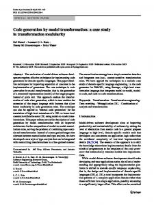
March 8th 2004 0

20

Fig. 2. Variable usage in the CPF Jacobian code VE-SLP-F. Each row corresponds to a statement and its entries indicate the statements that calculated the values of the variables involved.

40

60

80

100

120

140 0

20

40

60

80

100

120

140

rarely increases run time. We conclude that this is a very worthwhile strategy to use. 6.3.3 Depth-First Traversal (DFT) Statement Re-Ordering. The results with depth-first traversal (DFT) statement re-ordering (Section 6.1.4) were very mixed. Significant gains were sometimes made: ALPHA and AMD of Table III, PIII and AMD of Table IV, PIII and AMD of Table V. Sometimes significant losses were made: ALPHA, SGI of Table IV, Ultra10 of Table V. When successful, DFT appears to act as desired by reducing the number of memory operations performed. For example, in Table V the application of DFT re-ordering to the VE-SL-R subroutine to give VE-SL-R-DFT results in an 8% speed-up on the PIII platform. On examining the associated assembler we find that this is most likely to be due to a 14% drop in the number of loads and 8% drop in the number of stores. Conversely, on the Ultra10 platform we get a 21% reduction in efficiency on applying DFT and this is found to be associated with an undesired 27% increase in the number of stores. To understand how DFT reordering can reduce reads and writes to and from cache, consider the CPF problem with results of Table III. With only four exceptions, application of DFT reordering improves performance. Figures 2 and 3 show within which statements of the Jacobian codes VE-SLP-R and VE-SLP-R-DFT the variables are used. The first empty 29 rows in both plots correspond to the 11 independent variables and 18 constants (which are not calculated). Entries in columns 1 to 29 therefore denote uses of these variables and constants. In Figure 2, rows 30 to 62 correspond to the calculation of the function and local derivatives in the VESLP-R code; rows 63 to 87 correspond to the vertex elimination of intermediates from the function’s extended Jacobian; and rows 88 to 141 represent the assignment of the calculated scalar Jacobian entries to their matrix storage. Note that several columns are empty and correspond to variables unused in the right-hand side of any other statement e.g. assignments to the Jacobian. We see that the statements using a variable’s value are often widely separated from the statement that calculated ACM Transactions on Mathematical Software, Vol. 30, No. 3, Sep. 2004.

October 11, 2004


·

291

0

20

40

Fig. 3. Variable usage in the the DFT reordered CPF Jacobian code VE-SLP-F-DFT. Each row corresponds to a statement and its entries indicate the statements that calculated the values of the variables involved.

60

80

100

120

140 0

20

40

60

80

100

120

140

that value. For example, statement 141 uses the result of statement 86 - separated by 55 other statements. Unless the compiler itself performs significant reordering of the arithmetic instructions of the Jacobian code, then to keep all variables in registers between their calculation and last use will require a large number of registers. In Figure 3 we see that, with only a handful of exceptions, DFT reordering ensures entries of rows 30 to 141 lie either in the first 22 columns, corresponding to uses of independent variables and constants, or are clustered close to the diagonal corresponding to use of a value shortly after its calculation. Consequently if the independents are first read from cache and, together with the problem constants, kept in 22 registers throughout, then only a small number of other registers will be needed to avoid reads and writes to cache other than those necessary to store the function values and Jacobian entries. In a significant number of cases our best result (highlighted in bold) was obtained with a DFT code, which means that the technique should not be dismissed despite its mixed performance. The technique clearly needs improvement. Its most apparent weakness is that it fails to account for multiple uses of the independent variables and other constants. If, as in Figure 3, such uses are distributed throughout the code, and the numbers of such variables and constants is close to or exceeds the number of registers available, then performance will be impaired by the many loads and stores required. 6.3.4 Cross-Country Vertex Elimination. Only Table I shows operation count gains from cross-country vertex elimination that are other than negligible. In Table I, across all platforms, the best results were obtained by cross-country vertex elimination, sometimes aided by DFT statement re-ordering. Why it is only for the Roe case that cross-country elimination produces benefits demands some explanation. Table VI shows the number of entries in each of the blocks of the extended Jacobian as defined by equation (18) before and after pre-elimination. For the two sparse cases CTS and FIC of Sections 6.2.3 and 6.2.4, pre-elimination alone obtains the Jacobian in block R with other blocks then empty. ACM Transactions on Mathematical Software, Vol. 30, No. 3, Sep. 2004.

292

·


March 8th 2004

Table VI. Size and number of entries in blocks B, L, R and T of the extended Jacobians (equation (18)) for test cases differentiated at statement level. Figures in brackets are after reverse pre-elimination Size Number of entries in block m p B L R T Problem n Roe 10 5 62(36) 39(39) 140(88) 5(5) 14(37) HHD 8 8 18(18) 8(8) 16(16) 0(0) 68(68) 11 11 12(2) 12(1) 10(1) 38(49) 6(5) CPF 134 252 0(0) 0(0) 0(0) 882(882) 0(0) CTS 32 32 582(0) 582(0) 486(0) 16(246) 96(0) FIC

For the CPF problem of Section 6.2.2, pre-elimination eliminates all but 2 intermediates, so there can only be two subsequent, distinct elimination sequences for the statement-level differentiated code, namely forward and reverse orderings. This explains why use of the Markowitz and VLR heuristics leads to no improvement in the number of flops. After pre-elimination, the HHD problem of Section 6.2.1 still has 18 intermediates and so there is scope for the Markowitz and VLR heuristics to improve efficiency. A small reduction in nominal flops is obtained, though the two sequences are equivalent and performance is not significantly improved. However, for the Roe problem of Section 6.1, 36 intermediates and 88 entries in block L remain after pre-elimination. This greater complexity gives scope for the Markowitz and VLR heuristics to have a greater impact on the number of flops. Hence only for this case do the heuristics result in the most efficient Jacobian code, even so the improvement is small. 6.3.5 Code-List versus Statement-Level Differentiation. In Tables I-V we see that the pre-eliminated statement-level differentiated vertex-elimination codes always use fewer nominal flops and, in 38 of the 55 distinct problem/platform combinations (excluding DFT reorderings), out-perform the corresponding code-list differentiated codes. 6.4 Overall Performance of Vertex-Elimination AD Given the many variations in Jacobian code produced by EliAD (statementlevel or code-list differentiation, pre-elimination, elimination orderings and code re-orderings) it is useful to summarise the performance of the best EliAD generated Jacobian code with respect to the other calculation methods. Table VII gives the speed-up obtained in moving from 1-sided finite differencing (using row compression where applicable) to our best vertex elimination method for each problem and each platform. The inherent truncation error associated with finite differencing and the superior efficiency of factors between 1.7 to 11 for the EliAD generated code appear to justify use of elimination AD over finite differencing, though the efficiency of finite differencing would be improved by allowing the compiler to inline function calls. Table VIII gives the speed-up obtained in moving from the best conventional AD technique to our best vertex elimination method for each problem and each platform. Speed-ups of between 1.9 to 22.8 demonstrate the superiority of vertexelimination AD over conventional forward and reverse mode AD for Jacobian calculation. ACM Transactions on Mathematical Software, Vol. 30, No. 3, Sep. 2004.

October 11, 2004


·

293

Table VII. Speed-up of best vertex elimination AD over 1-sided finite differencing Platform Ultra10 PIII AMD Problem ALPHA SGI Roe 3.0 2.6 1.7 2.8 2.5 4.7 3.4 4.2 3.4 3.5 HHD CPF 11.0 9.2 7.8 7.3 6.4 8.2 8.0 6.9 4.6 10.4 CTS 7.2 6.2 5.5 7.2 6.9 FIC

Table VIII. Speed-up of best vertex elimination over best conventional AD Platform Problem ALPHA SGI Ultra10 PIII AMD Roe 2.0 2.3 1.9 2.1 1.9 HHD 5.9 5.7 5.8 4.5 4.0 4.5 4.4 5.9 3.2 3.9 CPF CTS 8.2 12.0 10.3 5.9 11.6 7.4 20.0 11.3 11.2 22.8 FIC

Table IX gives the speed-up obtained in moving from hand-coded Jacobian code Table IX. Speed-up of best vertex elimination AD over hand-coded Jacobian code Platform SGI Ultra10 PIII AMD Problem ALPHA HHD 1.13 1.05 1.50 0.69 0.76 1.49 1.62 2.02 1.22 1.26 CPF CTS 1.14 0.93 1.32 1.12 1.22 1.16 0.96 2.44 0.80 1.02 FIC

to our best vertex elimination method for the 4 problems for which we have handcoded Jacobians. Only for 5 of the 20 problem/platform combinations is handcoding superior, and for two of these the discrepancy is within 7%. 7. CONCLUSIONS AND PLANS FOR FUTURE WORK In this paper, we have presented the first extended set of results from EliAD, a source-transformation implementation of the vertex-elimination AD approach to Jacobian calculation of functions defined by Fortran code. Careful timings demonstrate an efficiency equal to that obtained by hand-coding and between 2 to 20 times superior to conventional AD techniques. This superiority is due to EliAD’s fuller exploitation of the sparsity of the extended Jacobian system that governs the relationship between the derivatives of all variables in the function code. Further, this exploitation of sparsity is performed at the Jacobian code generation stage, with statements generated only for those arithmetic operations involving nonzero entries in the extended Jacobian. Vertex elimination requires an ordering, or pivot sequence, in which to eliminate the derivatives of intermediate variables from the extended Jacobian. Monotonic inACM Transactions on Mathematical Software, Vol. 30, No. 3, Sep. 2004.

294

·


March 8th 2004

creasing and decreasing orderings correspond to sparsity-exploiting variants of conventional forward and reverse mode AD [Griewank and Reese 1991]. Consequently, vertex-elimination AD never uses more floating-point operations than conventional AD. The use of cross-country (i.e. non-monotonic) orderings gives further scope for reducing the number of floating-point operations. We have found that employing a pre-elimination strategy of eliminating any intermediate variable used only once, followed by a forward or reverse ordered elimination of all other intermediates, is very successful, both in reducing the number of floating-point operations and improving run-times. In the future, we wish to improve this strategy in the light of recent work [Naumann 2002b]. More involved ordering heuristics, such as the Markowitz and VLR strategies, were only worthwhile for one test case studied to date. Recently, elimination AD has been generalized to edge [Naumann 1999] and face [Naumann 2001; 2002a] eliminations, which may further reduce the number of flops required for Jacobian calculation. We are currently assessing these techniques for inclusion into EliAD. Interestingly, we found that reordering a Jacobian code’s statements frequently affected its performance. This appears to be due to changes in the number of loads and stores from cache to registers in the assembler of the reordered code. We are currently performing an in-depth study of the assembler produced for all the Jacobian codes of our study in order to get a better understanding of this issue and consequently improve both elimination heuristics and our code re-ordering strategy. For the sparse Jacobian cases (FIC and CTS), the EliAD generated Jacobian code was between 6 to 20 times more efficient than conventional AD using Jacobian compression. So, vertex-elimination AD appears excellently suited to least squares optimisation problems and numerical PDE solvers, where efficient Jacobian calculation enables fast solution via Newton-like solvers. To be more generally applicable for such problems requires removal of EliAD’s present restriction to loop-free code. This will greatly complicate EliAD’s activity analysis which will have to handle array indices as index ranges and not fixed values as at present. The techniques of [Tadjouddine et al. 1998; Tadjouddine 1999] will be modified to enable this. The ability to store such Jacobians in a suitable sparse matrix format will also be necessary. At the time of writing, EliAD’s functionality is being extended to include subprograms. A hierarchical approach utilising a conservative activity analysis of all variables in all possible branches and subroutines is adopted. This approach automates and generalises that of [Bischof and Haghighat 1996]. There are still many open questions related to the optimal calculation of Jacobians by elimination, both theoretical and implementational. Despite this, we feel certain that, with such issues now being studied in depth, the days of scientists and engineers painstakingly hand-coding Jacobian code to ensure efficiency are numbered.


October 11, 2004


·

295

APPENDICES A. PLATFORMS We ran test cases on COMPAQ ALPHA, Silicon Graphics and SUN UNIX machines with processor/compiler combinations denoted ALPHA, SGI and Ultra10. We also ran on two PC platforms with Pentium 3 and AMD Athlon processors. Relevant hardware data and the compiler information is given in Table X. Table X. Platform ALPHA SGI Ultra10 PIII AMD

Platform ALPHA SGI Ultra10 PIII/AMD

Platforms

a) Processors Processor CPU EV6 667MHz R12000 300MHz SUN Ultra10 440MHz Pentium 3 700MHz Athlon XP1800+ 1533MHz

L1-Cache 128KB 64KB 32KB 32KB 128KB

L2-Cache 8MB 8MB 2MB 256KB 256KB

b) Compilers Compiler Options Compaq f95 5.4 -O5 -fast -arch host -tune host f90 MIPSPro 7.3 -Ofast -IPA:inline=OFF -INLINE:none Workshop f90 6.0 -fast Compaq Visual Fortran /architecture:host /assume:noaccuracy sensitive /inline:manual /math library:fast /tune:host /opt:fast

B. TEST PROBLEM FUNCTION STATISTICS, CPU TIMES AND OPERATIONS COUNTS Table XI gives summary statistics for all 5 test problems. Columns p-SL and p-CL refer to the number of (active) intermediate variables in each function’s original statements and in its code-list respectively. Table XI. Summary statistics for test problem functions Problem n m p-SL p-CL Roe 10 5 62 208 8 8 20 84 HHD 11 11 13 57 CPF CTS 134 252 0 1386 32 32 680 1328 FIC

Table XII gives Nevals , the number of distinct Jacobians calculated, and Nrepet the number of times these calculations were repeated, in order to obtain reliable Jacobian timings. The second column of Table XIII gives the nominal computational cost W (f (x)) of calculating the test problems described in Section 6. It is determined by counting the number of floating operations within the Fortran code using a simple PERL ACM Transactions on Mathematical Software, Vol. 30, No. 3, Sep. 2004.

296

·


March 8th 2004

Table XII.

Values of Nevals and Nrepet used for each problem and platform Nevals Nrepet ALPHA, PIII & ALPHA SGI & PIII AMD SGI & AMD Ultra10 Ultra10 Problem Roe 500 60 2000 2000 16667 16667 HHD 2500 312 400 400 3200 12800 1000 125 2000 500 4000 16000 CPF 1 1 12000 12000 12000 120000 CTS 200 25 100 100 6400 6400 FIC

Table XIII. Nominal floating-point operations counts W (f ), lines of code (l.o.c.) and CPU times for test problem functions W (f ) Function CPU time(µs) (flops) l.o.c. ALPHA SGI Ultra10 PIII AMD Problem Roe 222 139 0.475 0.951 0.806 0.880 0.336 HHD 84 68 0.121 0.224 0.206 0.231 0.0943 68 45 0.351 0.870 0.503 0.495 0.162 CPF 1638 535 1.18 3.16 2.25 2.49 0.981 CTS FIC 1266 759 1.53 2.93 2.99 1.94 0.878

script. Table XIII also gives the number of non-comment lines of code (l.o.c.) and the average CPU times required to calculate the test problem functions f (x), as measured using the CPU TIME intrinsic function of the Fortran 95 programming language. Acknowledgements We thank Neil Stringfellow and Venkat Sastry for their help in developing the PERL scripts used in this paper and the three anonymous referees for the great care with which they read our paper and for their many suggestions.


October 11, 2004


·

297

REFERENCES Aho, A. V., Sethi, R., and Ullman, J. D. 1995. Compilers: Principles, Techniques, and Tools. Addison-Wesley, Reading, Mass. ´, J. J., and Xue, G.-L. 1992. The MINPACKAverick, B. M., Carter, R. G., More 2 test problem collection. Preprint MCS–P153–0692, ANL/MCS–TM–150, Rev. 1, Mathematics and Computer Science Division, Argonne National Laboratory, Argonne, Ill. See ftp://info.mcs.anl.gov/pub/MINPACK-2/tprobs/P153.ps.Z. Bendtsen, C. and Stauning, O. 1996. FADBAD, a flexible C++ package for automatic differentiation. Technical Report IMM-REP-1996-17, Technical University of Denmark, IMM, Departement of Mathematical Modeling, Lyngby. Berz, M., Bischof, C., Corliss, G., and Griewank, A., Eds. 1996. Computational Differentiation: Techniques, Applications, and Tools. SIAM, Philadelphia, Penn. ¨cker, H., Lang, B., Rasch, A., and Vehreschild, A. 2002. Combining source Bischof, C., Bu transformation and operator overloading techniques to compute derivatives for MATLAB programs. In Proceedings of the Second IEEE International Workshop on Source Code Analysis and Manipulation (SCAM 2002). IEEE Computer Society, p. 65–72. Bischof, C. H. 1991. Issues in parallel automatic differentiation. See Griewank and Corliss [1991], 100–113. Bischof, C. H., Carle, A., Hovland, P. D., Khademi, P., and Mauer, A. 1998. ADIFOR 2.0 user’s guide (Revision D). Tech. rep., Mathematics and Computer Science Division Technical Memorandum no. 192 and Center for Research on Parallel Computation Technical Report CRPC-95516-S. See www.mcs.anl.gov/adifor. Bischof, C. H., Carle, A., Khademi, P., and Mauer, A. 1996. ADIFOR 2.0: Automatic differentiation of Fortran 77 programs. IEEE Computational Science & Engineering 3, 3, 18–32. Bischof, C. H. and Haghighat, M. R. 1996. Hierarchical approaches to automatic differentiation. See Berz et al. [1996], 83–94. Bischof, C. H., Khademi, P. M., Bouaricha, A., and Carle, A. 1996. Efficient computations of gradients and Jacobians by dynamic exploitation of sparsity in automatic differentiation. Optimization Methods and Software 7, 1–39. Bischof, C. H., Roh, L., and Mauer, A. 1997. ADIC — An extensible automatic differentiation tool for ANSI-C. Software – Practice and Experience 27, 12, 1427–1456. See www-fp.mcs.anl. gov/division/software. ´, J. J. 1984. Software for estimating sparse Jacobian Coleman, T. F., Garbow, B. S., and More matrices. ACM Trans. Math. Software 10, 3, 329–345. Coleman, T. F. and Verma, A. 1998. ADMAT: An automatic differentiation toolbox for MATLAB. Tech. rep., Computer Science Department, Cornell University. ¨t, L., and Naumann, U., Eds. 2001. AutoCorliss, G., Faure, C., Griewank, A., Hascoe matic Differentiation: From Simulation to Optimization. Computer and Information Science. Springer, New York. Duff, I., Erisman, A. M., and Reid, J. 1989. Direct methods for sparse matrices. Monographs on numerical analysis. Oxford University Press. Faure, C. and Papegay, Y. 1998. Odyssée User’s Guide. Version 1.7. Rapport technique RT– 0224, INRIA, Sophia-Antipolis, France. Sept. See www.inria.fr/RRRT/RT-0224.html, and www. inria.fr/safir/SAM/Odyssee/odyssee.html. Forth, S. A. 2001. User guide for MAD - a Matlab automatic differentiation toolbox. Applied Mathematics and Operational Research Report AMOR 2001/5, Cranfield University (RMCS Shrivenham), Swindon, SN6 8LA, UK. June. Forth, S. A. and Tadjouddine, M. 2003. CFD Newton solvers with EliAD, an elimination automatic differentiation tool. In Computational Fluid Dynamics 2002: Proceedings of the Second International Conference on Computational Fluid Dynamics, ICCFD, S. Armfield, P. Morgan, and K. Srinivas, Eds. Springer, Sydney, Australia, 134–139. ACM Transactions on Mathematical Software, Vol. 30, No. 3, Sep. 2004.

298

·


March 8th 2004

Giering, R. and Kaminski, T. 1998. Recipies for adjoint code construction. ACM Trans. Math. Software 24, 4, 437–474. Also appeared as Max-Planck Institut f¨ ur Meteorologie Hamburg, Technical Report No. 212, 1996. Goedecker, S. and Hoisie, A. 2001. Performance Optimisation of Numerically Intensive Codes. Software, Environments, Tools. SIAM, Philadelphia. ISBN 0-89871-482-3. Griewank, A. 2000. Evaluating Derivatives: Principles and Techniques of Algorithmic Differentiation. Number 19 in Frontiers in Appl. Math. SIAM, Philadelphia, Penn. Griewank, A. and Corliss, G. F., Eds. 1991. Automatic Differentiation of Algorithms: Theory, Implementation, and Application. SIAM, Philadelphia, Penn. Griewank, A., Juedes, D., and Utke, J. 1996. ADOL–C, a package for the automatic differentiation of algorithms written in C/C++. ACM Trans. Math. Software 22, 2, 131–167. Griewank, A. and Reese, S. 1991. On the calculation of Jacobian matrices by the Markowitz rule. See Griewank and Corliss [1991], 126–135. Hascoet, L., Naumann, U., and Pascual, V. 2003. TBR analysis in reverse mode automatic differentiation. In Future Generation Computer Systems. Elsevier. Hovland, P. D. and McInnes, L. C. 2001. Parallel simulation of compressible flow using automatic differentiation and PETSc. Parallel Computing 27, 4 (March), 503–519. Knuth, D. E. 1997. The Art of Computer Programming, Volume 1: Fundamental Algorithms. Adison-Wesley. Markowitz, H. 1957. The elimination form of the inverse and its application. Management Science 3, 257–269. Naumann, U. 1999. Efficient calculation of Jacobian matrices by optimized application of the chain rule to computational graphs. Ph.D. thesis, Technical University of Dresden. Naumann, U. 2001. Elimination techniques for cheap Jacobians. See Corliss et al. [2001], Chapter 29, 241–246. Naumann, U. 2002a. Elimination methods in computational graphs. on the optimal accumulation of Jacobian matrices- conceptual framework. Mathematical Programming. (Submitted). Naumann, U. 2002b. On optimal Jacobian accumulation for single expression use programs. Mathematical Programming. (Submitted). Parr, T., Lilly, J., Wells, P., Klaren, R., Illouz, M., Mitchell, J., Stanchfield, S., Coker, J., Zukowski, M., and Flack, C. 2000. ANTLR Reference Manual. Tech. rep., MageLang Institute’s jGuru.com. January. See www.antlr.org/doc/index.html. Pryce, J. D. and Reid, J. K. 1998. ADO1, a Fortran 90 code for automatic differentiation. Tech. Rep. RAL-TR-1998-057, Rutherford Appleton Laboratory, Chilton, Didcot, Oxfordshire, OX11 OQX, England. See ftp://matisa.cc.rl.ac.uk/pub/reports/prRAL98057.ps.gz. Reid, J. 2003. On the stability of automatic differentiation. To appear . Roe, P. L. 1981. Approximate Riemann solvers, parameter vectors, and difference schemes. Journal of Computational Physics 43, 357–372. Tadjouddine, M. 1999. La différentiation automatique. Ph.D. thesis, Université de Nice, Sophia Antipolis, France. Tadjouddine, M., Eysette, F., and Faure, C. 1998. Sparse Jacobean computation in automatic differentiation by static program analysis. In Proceedings of the Fifth International Static Analysis Symposium. Number 1503 in Lecture Notes in Computer Science. Springer-Verlag, Pisa, Italy, 311–326. Tadjouddine, M., Forth, S. A., and Pryce, J. D. 2001. AD tools and prospects for optimal AD in CFD flux Jacobian calculations. See Corliss et al. [2001], Chapter 30, 247–252. Tadjouddine, M., Forth, S. A., and Pryce, J. D. 2003. Hierarchical automatic differentiation by vertex elimination and source transformation. In Computational Science and its Applications - ICCSA 2003. Lecture Notes in Computer Science, vol. 2. Springer-Verlag, Montreal, 115–124. Tadjouddine, M., Forth, S. A., Pryce, J. D., and Reid, J. K. 2002. Performance issues for vertex elimination methods in computing Jacobians using automatic differentiation. In Proceedings of the Second International Conference on Computational Science, P. M. Sloot, Ed. Lecture Notes in Computer Science, vol. 2. Springer-Verlag, Amsterdam, 1077–1086. ACM Transactions on Mathematical Software, Vol. 30, No. 3, Sep. 2004.

October 11, 2004


·

299

Verma, A. 1998. ADMAT: Automatic differentiation in MATLAB using object oriented methods. In SIAM Interdisciplinary Workshop on Object Oriented Methods for Interoperability. SIAM, National Science Foundation, Yorktown Heights, New York, 174–183. Wilkinson, J. 1965. The Algebraic Eigenvalue Problem. Oxford University Press. Received Dec 2002; revised October 2003; revised February 2004; accepted March 2004.


Jacobian Code Generated by Source Transformation and ... - CiteSeerX

Jacobian Code Generated by Source Transformation and ... - CiteSeerX

Suggest Documents

Jacobian Code Generated by Source Transformation ...

Jacobian Code Generated by Source Transformation ...

Jacobian Code Generated by Source ... - Semantic Scholar

Model Checking DSL-Generated C Source Code

adjoint code by source transformation with openad/f - Semantic Scholar

Executable source code and non-executable source code ... - CiteSeerX

1 Source code transformation using Rubus - Plos

Combining source transformation and operator ... - CiteSeerX

Combining source transformation and operator ... - CiteSeerX

Combining source transformation and operator ... - CiteSeerX

Towards Model Transformation in Generated Eclipse ... - CiteSeerX

Improving Source Code Locality - CiteSeerX

Improving Source Code Locality - CiteSeerX

Source Code Plagiarism Detection - CiteSeerX

Error-correcting Source Code - CiteSeerX

Source Code Repositories and Agile Methods - CiteSeerX

Source Code for Biology and Medicine - CiteSeerX

Source Code for Biology and Medicine - CiteSeerX

Code generation by model transformation: a case study in ... - CiteSeerX

Refactoring by Transformation - CiteSeerX

Predicting Source Code Changes by Mining Revision ... - CiteSeerX

Verification of Source Code Transformations by Program ... - CiteSeerX

Verification of Source Code Transformations by Program ... - CiteSeerX

Clone Detection in Source Code by Frequent Itemset ... - CiteSeerX