Join Optimization of Information Extraction Output: Quality ... - CiteSeerX

Join Optimization of Information Extraction Output: Quality Matters! Alpa Jain1 , Panagiotis Ipeirotis2 , AnHai Doan3 , Luis Gravano1 1

Columbia University, 2 New York University, 3 University of Wisconsin-Madison

Abstract— Information extraction (IE) systems are trained to extract specific relations from text databases. Real-world applications often require that the output of multiple IE systems be joined to produce the data of interest. To optimize the execution of a join of multiple extracted relations, it is not sufficient to consider only execution time. In fact, the quality of the join output is of critical importance: unlike in the relational world, different join execution plans can produce join results of widely different quality whenever IE systems are involved. In this paper, we develop a principled approach to understand, estimate, and incorporate output quality into the join optimization process over extracted relations. We argue that the output quality is affected by (a) the configuration of the IE systems used to process documents, (b) the document retrieval strategies used to retrieve documents, and (c) the actual join algorithm used. Our analysis considers several alternatives for these factors, and predicts the output quality—and, of course, the execution time— of the alternate execution plans. We establish the accuracy of our analytical models, as well as study the effectiveness of a qualityaware join optimizer, with a large-scale experimental evaluation over real-world text collections and state-of-the-art IE systems.

Company

MergedWith

Microsoft

Softricity

Microsoft

Symantec

CEO

Steve Ballmer Steve Ballmer Executives

Mergers Company

?

MergedWith

Microsoft

Softricity

Microsoft

Microsoft

Symantec

Merck

Microsoft

aQuantive

Apple

SeekingAlpha

Fig. 1.

Company

CEO Steve Ballmer Richard Clark

Vadim Zlotnikov

The Wall Street Journal

Joining information derived from multiple extraction systems.

Example 1: Consider two text databases, the blog entries from SeekingAlpha (SA), a highly visible blog that discusses financial topics, and the archive of The Wall Street Journal (WSJ) newspaper. These databases embed information that can be used to answer a financial analyst’s query (e.g., expressed in SQL) asking for all companies that recently merged, including information on their CEOs (see Figure 1). To answer such a query, we can use IE systems to extract a MergersCompany, I. I NTRODUCTION MergedWith relation from SA and an ExecutivesCompany, Many unstructured text documents contain valuable data that CEO relation from WSJ. For Mergers, we extract tuples such as can be represented in structured form. Information extraction Microsoft, Softricity, indicating that Microsoft merged with (IE) systems automatically extract and build structured relations Softricity; for Executives, we extract tuples such as Microsoft, from text documents, enabling the efficient use of such data Steve Ballmer, indicating that Steve Ballmer has been a CEO in relational database systems. Real-world IE systems and of Microsoft. After joining all the extracted tuples, we can architectures, such as Avatar1 , DBLife2 , and UIMA [7], view construct the information sought by the analyst. Unfortunately, IE systems as blackboxes and “stitch” together the output from the join result is far from perfect. As shown in Figure 1, the multiple such blackboxes to produce the data of interest. A IE system for Mergers incorrectly extracted tuple Microsoft, common operation at the heart of these multi-blackbox systems Symantec, and failed to extract tuple Microsoft, aQuantive. is thus joining the output from the IE systems. Accordingly, Missing or erroneous tuples, in turn, hurt the quality of join recent work [7], [11], [17] has started to study this important results. For example, the erroneous tuple Microsoft, Symantec problem of processing joins over multiple IE systems. is joined with the correct tuple Microsoft, Steve Ballmer Just as in traditional relational join optimization, efficiency from the Executives relation to produce an erroneous join tuple is, of course, important when joining the output of multiple Microsoft, Symantec, Steve Ballmer.  IE systems. Existing work [7], [17] has thus focused on this A key observation that we make in this paper is that different aspect of the problem, which is critical because IE can be timejoin execution plans for extracted relations can differ vastly in consuming (e.g., it often involves expensive text processing their output quality. Therefore, considering the expected output operations such as part-of-speech and named-entity tagging). quality of each candidate plan is of critical importance, and is Unlike in the relational world, however, the join output quality at the core of this paper. The output quality of a join execution is of critical importance, because different join execution plans plan depends on (a) the configuration and characteristics of the might differ drastically in the quality of their output. Several IE systems used by the plan to process the text documents, and factors influence the output quality, as we discuss below. The (b) the document retrieval strategies used by the plan to retrieve following example highlights one such factor, namely, how the documents for extraction. Previous work has recognized errors by individual IE systems impact the join output quality. the importance of output quality for single relations [10], [8]. 1 http://www.almaden.ibm.com/cs/projects/avatar Recent work [11] has also considered these two factors for 2 http://www.dblife.cs.wisc.edu choosing a join execution plan over multiple extracted relations.

Unfortunately, earlier work has failed to consider a third, II. R ELATED W ORK important factor, namely, (c) the choice of join algorithm. Information extraction from text has received much attention In this paper, we introduce and analyze three fundamentally in the database, AI, Web, and KDD communities (see [3], [6] different join execution algorithms for information extraction for tutorials). The majority of the efforts have considered the tasks, which differ in the extent of interaction between the construction of a single extraction system that is as accurate as extraction of the relations (e.g., from independent extraction to possible (e.g., using HMMs and CRFs [3], [14]). Approaches a completely interleaved extraction), or in the way we retrieve to improve the efficiency of the IE process have developed and process database documents (e.g., scan- or query-based specialized document retrieval strategies; one such approach retrieval). Our analysis reveals that the choice of join algorithm is the QXtract system [2], which uses machine learning to plays a crucial role in determining the overall output quality derive keyword queries that identify documents rich in target of a join execution plan, just as this choice crucially affects information. We use QXtract in our work. execution time in a relational model setting. We will see that Our earlier work [10], [12] studied the task of extracting even a simple two-way join has a vast execution plan space, just one relation, not our join problem. Specifically, in [10] with each execution plan exhibiting unique output quality and we studied the document retrieval strategies considered in this execution efficiency characteristics. paper for the goal of efficiently achieving a desired recall for a Understanding how join algorithms work, in concert with single-relation extraction task. The analysis in [10] assumes a other factors such as the choice of extraction systems and their perfect IE system (i.e., all generated tuples are good). On the configurations, and the choice of document retrieval strategies, other hand, in [12] we studied document retrieval strategies is thus crucial to optimize the processing of a join query. for single-relation extraction while accounting for extraction During optimization, we need to answer challenging questions: imprecision. Our current work builds upon the statistical models How should we configure the underlying IE systems? What presented in [10], [12], extending them for multiple IE systems. is the correct balance between precision and recall for the Real-world applications often require multiple IE systems [6], IE systems? Should we retrieve and process all the database [17]. Hence, the problem of developing and optimizing IE documents, or should we selectively retrieve and process only programs that consist of multiple IE systems has received a small subset? What join execution algorithm should we use, growing attention [16]. Some of the existing solutions write and what is the impact of this choice on the output quality? To such programs as declaratively as possible (e.g., UIMA [7], answer these questions, we derive equations for the execution GATE [5], Xlog [17]), while considering only the execution efficiency and output quality of a join execution plan as a time in their analysis. function of the choice of IE systems and their configurations, In prior work [11], we presented a query optimization apthe choice of document retrieval strategies, and the choice proach for simple SQL queries involving joins while accounting of join algorithm. To the best of our knowledge, this paper for both execution time and output quality. Our earlier paper presents the first holistic, in-depth study—incorporating all the considered only one simple heuristic to estimate the quality above factors—of the output quality of join execution plans. of one simple join algorithm, namely, the IDJN algorithm, A substantial challenge that we also address is defining and discussed and analyzed in this paper (Section IV). Our current extracting appropriate, comprehensive database statistics to work substantially expands on [11] by modeling an extended guide the join optimization process in a quality-aware manner. family of join algorithms and showing how to pick the best As a key contribution of this paper, we show how to build option dynamically. To the best of our knowledge, our current rigorous statistical inference techniques to estimate the param- work is the first to carry out an in-depth output quality analysis eters necessary for our analytical models of output quality; of a variety of join execution plans over multiple IE systems. furthermore, our parameter estimation happens efficiently, onIII. U NDERSTANDING J OIN Q UALITY the-fly during the join execution. As another key contribution, In this section, we provide background on the problem of we develop an end-to-end, quality-aware join optimizer that adaptively changes join execution strategies if the available joining relations extracted from text databases. We discuss important aspects of the problem that affect the overall quality statistics suggest that a change is desirable. of the join results. We define the family of join execution plans In summary, the main contributions of this paper are: that we consider, as well as user-specified quality preferences. • We introduce a principled approach to estimate the output quality of a join execution and incorporate quality into the A. Tuning Extraction Systems: Impact on Extraction Quality join optimization process over multiple extracted relations. Extraction is a noisy process, and the extracted relations • We present an end-to-end, quality-aware join optimization may contain erroneous tuples or miss valid tuples. An extracted approach based on our analytical models, as well as effec- relation can be regarded as consisting of good tuples, which tive methods to estimate all necessary model parameters. are the correctly extracted tuples, and bad tuples, which are the • We establish the accuracy of our output quality models erroneous tuples. For instance, in Figure 1, Mergers consists and the effectiveness of our join optimization approach of one good tuple, Microsoft, Softricity, and one bad tuple, through an extensive experimental evaluation over real-life Microsoft, Symantec. To control the quality of such extracted text collections and state-of-the-art IE systems. relations, IE systems often expose multiple tunable “knobs”

that affect the proportion of good and bad tuples in the IE We now show that we can leverage these single-relation output. These knobs may be decision thresholds, such as the document retrieval strategies to develop join execution plans minimum confidence required before generating a tuple from involving multiple extracted relations. text. We denote a particular configuration of such IE-specific knobs by θ. In our earlier work [15], we showed how we can C. Choosing Join Execution Plans: User Preferences and robustly characterize the effect of such knob settings for an Impact on Extraction Quality In this paper, we focus on binary natural joins, involving two individual IE system, which we briefly review next. Specifically, given a knob configuration θ for an IE system, we can capture extracted relations; we leave higher order joins as future work. the effect of θ over a database D using two values: (a) the As discussed above, and unlike in the relational world, different true positive rate tp(θ) is the fraction of good tuples that join execution plans in our text-based scenario can differ not appear in the IE output over all the good tuples that could be only in their execution time, but also in the quality of the join extracted from D with the IE system across all possible knob results that they produce. The output quality and, of course, configurations, while (b) the false positive rate fp(θ) is the the execution time is affected by (a) the configuration of the IE fraction of bad tuples that appear in the IE output over all the systems used to process the database documents, as argued in bad tuples that could be extracted from D with the IE system Section III-A, and (b) the document retrieval strategies used to across all possible knob configurations. To define tp(θ) and select the documents for processing, as argued in Section III-B. fp(θ) we need to know the sets of all possible good and bad Interestingly, (c) the choice of join algorithms also has an tuples, which serve as normalizing factors for tp(θ) and fp(θ), impact on the output quality and execution time, as we will respectively. In practice, we estimate tp(θ) and fp(θ) using a see. We thus define a join execution plan as follows: Definition 3.1: [Join Execution Plan] Consider two development set of documents and “ground truth” tuples [12]. databases D1 and D2 , as well as two IE systems E1 and E2 . B. Choosing Document Retrieval Strategies: Impact on Extrac- Assume Ei is trained to extract relation Ri from Di (i = 1, 2). tion Quality  R2 is a tuple A join execution plan for computing R1  Analogous to the above classification of the tuples extracted E1 θ1 , E2 θ2 , X1 , X2 , JN , where θi specifies the knob by an IE system E from a database D, we can classify each configuration of Ei (see Section III-A) and Xi specifies the document in D with respect to E as a good document, if E document retrieval strategy for Ei over Di (see Section III-B), can extract at least one good tuple from the document, as a bad for i = 1, 2, while JN is the choice of join algorithm for the document, if E can extract only bad tuples from the document, execution, as we will discuss below.  Given a join execution plan S over databases D1 and D2 , or as an empty document, if E cannot extract any tuples— good or bad—from the document. Ideally, when processing the execution time Time(S, D1 , D2 ) is the total time required a text database with an IE system, we should focus on good for S to generate the join results from D1 and D2 . We identify documents and process as few empty documents as possible, the important components of execution time for different join for efficiency reasons; we should also process as few bad execution plans in Section V, where we will also analyze the documents as possible, for both efficiency and output quality output quality associated with each plan. We now introduce some additional notation that will be reasons. To this end, several document retrieval strategies have needed in our output-quality analysis in the remainder of the been introduced in the literature [10], [11]: paper. Recall from Section III-A that the tuples that an IE Scan (SC) sequentially retrieves and processes each document system extracts for a relation can be classified as good tuples or in a database. While this strategy is guaranteed to process all bad tuples. Analogously, we can also classify the attribute value good documents, it also processes all the empty and bad ones, occurrences in an extracted relation according to the tuples and may then introduce many bad tuples. where these values occur. Specifically, consider an attribute Filtered Scan (FS) is another scan-based strategy; instead value a and a tuple t in which a appears. We say that the of processing all available documents, FS uses a document occurrence of a in t is a good attribute value occurrence if t is classifier to decide whether a document is good or not. FS a good tuple; otherwise, this is a bad attribute value occurrence. avoids processing all documents, and thus tends to have fewer Note that an attribute value might have both good and bad bad tuples in the output. However, since the classifier may also occurrences. For instance, in Figure 1 the value “Microsoft” has erroneously reject good documents, FS might not include all both a good occurrence in (good) tuple Microsoft, Softricity the good tuples in the output. and a bad occurrence in (bad) tuple Microsoft, Symantec. Automatic Query Generation (AQG) is a query-based strat- We denote the set of good attribute value occurrences for an egy that issues (automatically generated [2]) queries to the extracted relation Ri by Agi and the set of bad attribute value database that are expected to retrieve good documents. For occurrences by Abi . Consider now a join R1   R2 over two extracted relations example, AQG may derive—using machine learning—the query [“executive” AND “announced”] to retrieve documents for R1 and R2 . Just as in the single-relation case, the join the Executives relation (see Example 1). This strategy avoids TR1  R2 contains good and bad tuples, denoted as Tgood  processing all the documents, but might not include all the and Tbad  , respectively. The tuples in Tgood  are the result of joining only good tuples from the base relations; all good tuples in the output.

R1

R2

a b c e a b c d e

R1

Fig. 2.

a x b c e e

R2

Composition of R1   R2 from extracted relations R1 and R2 .

Input: number of good tuples τg , number of bad tuples τb , E1 θ1 , E2 θ2  Output: R1   R2 Rj = ∅ /* tuples produced for R1   R2 */ Tr 1 = ∅, Tr 2 = ∅ /* tuples extracted for R1 and R2 */ Dr 1 = ∅, Dr 2 = ∅ /* documents retrieved from D1 and D2 */ while {estimated # good tuples in Rj < τg } AND {estimated # bad tuples in Rj ≤ τb } do if |Dr 1 | < |D1 | then Retrieve an unseen document d from D1 and add to Dr 1 Process d using E1 at θ1 to generate tuples t1 end if |Dr 2 | < |D2 | then Retrieve an unseen document d from D2 and add to Dr 2 Process d using E2 at θ2 to generate tuples t2 end Tjoin = (t1   t2 ) ∪ (Tr 1   t2 ) ∪ (t1   Tr 2 ) Tr 1 = Tr 1 ∪ t1 Tr 2 = Tr 2 ∪ t2 Rj = Rj ∪ Tjoin if {|Dr 1 | = |D1 |} AND { |Dr 2 | = |D2 |} then return Rj end end return Rj

other combinations result in bad tuples. Figure 2 illustrates this point using example relations R1 and R2 , with 2 good and 3 bad tuples each. In this figure, we have Ag1 = {a, c} and Ab1 = {b, d, e} for relation R1 , and Ag2 = {a, b} and Ab2 = {x, c, e} for relation R2 . The composition of the join Fig. 3. The IDJN algorithm using Scan. tuples yields |Tgood  | = 3.  | = 1 and |Tbad User Preferences: In our IE-based scenario, there is a natural   trade-off between output quality and execution efficiency. Some join execution plans might produce “quick-and-dirty” results,  while other plans might result in high-quality results that require  Fig. 4. Exploring D1 × D2 with IDJN using Scan. a long time to produce. Ultimately, the right balance between quality and efficiency is user-specific, so our query model estimate that the quality requirements cannot be met, in which includes such user preferences as an important feature. One case the join optimizer may build on the current execution with approach for handling these user preferences, which we follow a different join execution plan or, alternatively, discard any in this paper, is for users to specify the desired output quality— produced results and start a new execution plan from scratch which should be reached as efficiently as possible—in terms (see Section VI). of the minimum number τg of good tuples that they request, together with the maximum number τb of bad tuples that they A. Independent Join 3 can tolerate, so that |Tgood  | ≤ τb .  | ≥ τg and |Tbad The Independent Join algorithm (IDJN) [11] computes a Other cost functions can be designed on top of this lower binary join by extracting the two relations independently and level model: examples include minimum precision at top-k then joining them to produce the final output. To extract each results, minimum recall at the end of the execution, or a goal relation, IDJN retrieves the database documents by choosing to maximize a weighted combination of precision and recall from the document retrieval strategies in Section III-A, namely, within a pre-specified execution time budget. For conciseness Scan, Filtered Scan, and Automatic Query Generation. and clarity, in our work the user quality requirements are Figure 3 describes the IDJN algorithm for the settings of expressed in terms of τg and τb , as discussed above. Definition 3.1 and for the case where the document retrieval strategy is Scan. IDJN receives as input the user-specified IV. J OIN A LGORITHMS FOR E XTRACTED R ELATIONS output quality requirements τg and τb (see Section III), and As argued above, the choice of join algorithm is one of the the relevant extraction systems E1 θ1  and E2 θ2 . IDJN key factors affecting the result quality. We now briefly discuss sequentially retrieves documents for both relations, runs the three alternate join algorithms, which we later analyze in terms extraction systems over them, and joins the newly extracted of their output quality and execution efficiency. Following tuples with all the tuples from previously seen documents. Section III-C, each join algorithm will attempt to meet the Conceptually, the join algorithm can be viewed as “traversing” user-specified quality requirements as efficiently as possible. the Cartesian product D1 × D2 of the database documents, This goal is then related to that of ripple joins [9] for online as illustrated in Figure 4: the horizontal axis represents the aggregation, which minimize the time to reach user-specified documents in D1 , the vertical axis represents the documents performance requirements. Our discussion of the alternate join in D2 , and each element in the grid represents a document algorithms builds on the ripple join principles. pair in D1 × D2 , with a dark circle indicating an already As we will see, the join algorithms base their stopping visited element. (The documents are displayed in the order of conditions on the user-specified quality requirements, given retrieval.) Figure 4 shows a “square” version of IDJN, which as τg and τb bounds on the number of good and bad tuples retrieves documents from D1 and D2 at the same rate; we can in the join output. Needless to say, the join algorithms do generalize this algorithm to a “rectangle” version that retrieves not have any a-priori knowledge of the correctness of the documents from the databases at different rates. extracted tuples, so the algorithms will rely on estimates to The number of documents to explore will depend on the decide when the quality requirements have been met (see user-specified values for τg and τb , and also on the choice of Section V). Also, during execution a join algorithm might the retrieval strategies for each relation. When using Filtered Scan, we may filter out a retrieved document from a database 3 A natural alternative formulation is to specify the desired output quality and, as a result, some portion of D1 × D2 will remain as percentages of the total number of tuples [10]. 







Input: number of good tuples τg , number of bad tuples τb , E1 θ1 , E2 θ2  Output: R1   R2 Rj = ∅ /* tuples produced for R1   R2 */ /* R1 is the outer relation and R2 is the inner relation */ Tr 1 = ∅, Tr 2 = ∅ /* tuples extracted for R1 and R2 */ Dr 1 = ∅, Dr 2 = ∅ /* documents retrieved from D1 and D2 */ while {estimated # good tuples in Rj < τg } AND {estimated # bad tuples in Rj ≤ τb } do Qs = ∅ /* queries for the inner relation */ Retrieve an unseen document d from D1 and add to Dr 1 Process d using E1 at θ1 to generate tuples t1 Generate keyword queries from t1 and add to Qs Tr 1 = Tr 1 ∪ t1 Rj = Rj ∪ (t1   Tr 2 ) foreach query q ∈ Qs do Issue q to D2 to retrieve unseen matching documents and add them to Dr 2 Process all unprocessed documents in Dr 2 using E2 at θ2 to generate tuples t2 Tr 2 = Tr 2 ∪ t2 Rj = Rj ∪ (Tr 1   t2 ) end if |Dr 1 | = |D1 | then return Rj end end return Rj

Fig. 5.

The OIJN algorithm using Scan for the outer relation.

Input: number of good tuples τg , number of bad tuples τb , E1 θ1  and E2 θ2 , Qseed Output: R1   R2 Rj = ∅ /* tuples produced for R1   R2 */ Tr 1 = ∅, Tr 2 = ∅ /* tuples extracted from R1 and R2 */ Dr 1 = ∅, Dr 2 = ∅ /* documents retrieved from D1 and D2 */ Q1 = Qseed , Q2 = ∅ /* queries issued to D1 and D2 */ while Q1 = ∅ OR Q2 = ∅ do if Q1 = ∅ then Pull next query q1 out of Q1 Issue q1 to D1 to retrieve unseen matching documents and add them to Dr 1 Process all unprocessed documents in Dr 1 using E1 at θ1 to generate tuples t1 Generate keyword queries from t1 and append to Q2 Tr 1 = Tr 1 ∪ t1 Rj = Rj ∪ (t1   Tr 2 ) end if {estimated # good tuples in Rj ≥ τg } OR {estimated # bad tuples in Rj > τb } then return Rj end if Q2 = ∅ then Pull next query q2 out of Q2 Issue q2 to D2 to retrieve unseen matching documents and add them to Dr 2 Process all unprocessed documents in Dr 2 using E2 at θ2 to generate tuples t2 Generate keyword queries from t2 and append to Q1 Tr 2 = Tr 2 ∪ t2 Rj = Rj ∪ (Tr 1   t2 ) end if {estimated # good tuples in Rj ≥ τg } OR {estimated # bad tuples in Rj > τb } then return Rj end end

Fig. 7.





The ZGJN algorithm.

in the D1 × D2 space. 

(a) Fig. 6.



(b)

Exploring D1 × D2 with (a) OIJN and (b) ZGJN.

unexplored. Similarly, when using Automatic Query Generation, the maximum number of documents retrieved from a database may be limited, resulting in a similar effect. B. Outer/Inner Join The IDJN algorithm does not effectively exploit any existing keyword-based indexes on the text databases. Existing indexes can be used to guide the join execution towards processing documents likely to contain a joining tuple. The next join algorithm, Outer/Inner Join (OIJN), shown in Figure 5, corresponds to a nested-loop join algorithm in the relational world. OIJN thus picks one of the relations as the “outer” relation and the other as the “inner” relation. (Our analysis in Section V can be used to identify which relation should serve as the outer relation in a join execution.) OIJN retrieves documents for the outer relation using one of the document retrieval strategies and processes them using an appropriate extraction system. OIJN then generates keyword queries using the values for the joining attributes in the extracted outer relation. Using these queries, OIJN retrieves and processes documents for the inner relation that are likely to contain the “counterpart” for the already seen outer-relation tuples. Figure 6(a) illustrates the traversal through D1 × D2 for the OIJN algorithm: each querying step corresponds to a complete probe of the inner relation’s database, which sweeps out an entire row of D1 × D2 . Thus, OIJN effectively traverses the space, biasing towards documents likely to contain joining tuples from the inner relation, which may result in an efficient refinement over IDJN. However, the maximum number of documents that can be retrieved via a query may be limited by the search interface, which, in turn, limits the maximum number of tuples retrieved using OIJN. The impact of this limit on the number of matching documents is denoted in Figure 6(a) as gray circles that depict some unexplored area

C. Zig-Zag Join The Zig-Zag Join (ZGJN) algorithm generalizes the idea of using keyword queries from OIJN, so that we can now query for both relations and interleave the extraction of the two relations; see Figure 7. Starting with one tuple extracted for one relation, ZGJN retrieves documents—via keyword querying on the join attribute values—for extracting the second relation. In turn, the tuples from the second relation are used to build keyword queries to retrieve documents for the first relation, and the process iterates, effectively alternating the role of the “outer” relation of a nested-loop execution over the two relations. Conceptually, each step corresponds to a sweep of an entire row or column of D1 × D2 , as shown in Figure 6(b). Similarly to OIJN, ZGJN can efficiently traverse the D1 × D2 space; however, just as for OIJN, the space covered by ZGJN is limited by the maximum number of documents returned by the underlying search interface. V. E STIMATING J OIN Q UALITY Each join execution plan (Definition 3.1) produces join results whose quality depends on the choice of IE system— and their tuning parameters (see Section III-A)—, document retrieval strategies (see Section III-B), and join algorithms (see Section IV). We now turn to the core of this paper, where we present analytical models for the output quality of the join execution plans. Specifically, for each execution plan we derive formulas for the number |Tgood  | of good tuples and the  R2 that the plan number |Tbad  | of bad tuples in R1  produces, as a function of the number of documents retrieved and processed by the IE systems. A. Notation In the rest of the discussion, we consider two text databases, D1 and D2 , with two IE systems E1 and E2 , where extraction system Ei extracts relation Ri from Di (i = 1, 2). Table I summarizes our notation for the good, bad, and empty database documents, for the good and bad tuples and attribute values,

Symbol

Description

Ri Ei Xi

Extracted relations (i = 1, 2) Extraction system for Ri Document retrieval strategy for Ei

Di Dgi Dbi Dei Dr i

Database for extracting Ri Set of good documents in Di Set of bad documents in Di Set of empty documents in Di Set of documents retrieved from Di

Symbol

Description

Agi Abi gi (a) bi (a) Oi (a)

Good attribute values in Ri Bad attribute values in Ri Frequency of a in Dg i Frequency of a in Dbi Frequency of a in Dr i

TABLE I N OTATION SUMMARY.

as well as for their frequency in the extracted relations (see Section III-C). Additionally, for a natural join attribute A4 , we denote the attribute values common to both extracted relations R1 and R2 as follows: Agg = Ag1 ∩ Ag2 , Agb = Ag1 ∩ Ab2 , Abg = Ab1 ∩ Ag2 , and Abb = Ab1 ∩ Ab2 . In Figure 2, Agg = {a}, Agb = {c}, Abg = {b}, and Abb = {e}. B. Analyzing Join Execution Plans: General Scheme

In practice, we do not know the exact frequencies g1 (a) and g2 (a) for each attribute value. However, we can typically estimate the probability P r{gi } that an attribute value occurs gi times in an extracted relation, using parametric or nonparametric approaches (e.g., often the frequency distribution of attribute values follows a power law [10]). So, |Dg1 | |Dg2 |

E[|Tgood  |] = |Agg|·

 

E[gr1 |g1 ]·E[gr2 |g2 ]·P r{g1 , g2 }

g1 =1 g2 =1

The factor P r{g1 , g2 } is the probability that an attribute value has g1 good occurrences in D1 and g2 good occurrences in D2 . We make a simplifying independence assumption so that P r{g1 , g2 } = P r{g1 } · P r{g2 }. Alternatively, we could assume that frequent attribute values in one relation are commonly frequent in the other relation as well, and vice versa6 . In this scenario, we would have: P r{g1 } ≈ P r{g2 } and P r{g1 , g2 } ≈ P r{g1 } ≈ P r{g2 }.  R2 To compute the number |Tbad  | of bad tuples in R1  we proceed in the same fashion, with two main differences: we need to consider three different classes of attributes, namely, Agb, Abg, and Abb, and compute the expected number of bad attribute occurrences in an extracted relation. Specifically,

We begin our analysis by sketching a general scheme to study the output of an execution plan in terms of its number of good tuples |Tgood  |. In later  | and bad tuples |Tbad sections, we will instantiate this general scheme for the various join execution plans that we study. Consider relations R1 and R2 , to be extracted and joined over a single common attribute A, and let a be a value of |Tbad  | = Jgb + Jbg + Jbb join attribute A with g1 (a) good occurrences in D1 5 and g2 (a)   |Dg1 | |Db2 |   good occurrences in D2 . Suppose that a join execution retrieves where Jgb = |Agb| · g1 =1 b2 =1 E[gr 1 g1 ] · E[br 2 b2 ] · , b }. We can compute values for J and J using P r{g 1 2 bg bb documents Dr 1 from D1 and documents Dr 2 from D2 , and we observe gr1 (a) good occurrences of a in Dr 1 and gr2 (a) |Abg| and |Abb|, respectively, along with appropriate tuple good occurrences of a in Dr 2 . Then, the number of good cardinality values. Using this generic analysis along with the expected frequenjoin tuples with A = a is gr1 (a) · gr2 (a) (see Section III-C). cies for the attribute occurrences, we can derive the exact Generalizing this analysis to all good attribute occurrences  R2 . We now complete and instantiate composition of R1  common to both relations (i.e., to the values in Agg) the total this analysis for the alternate join algorithms of Section IV. number |Tgood  R2 is:  | of good tuples extracted for R1   C. Independent Join gr1 (a) · gr2 (a) (1) |Tgood | = Our goal is to derive the expected frequency E[gr i ] for good a∈Agg attribute occurrences and E[br i ] for bad attribute occurrences where Agg is the set of join attribute values with good after we have retrieved Dr i documents from Di , given in R i occurrences in both relations (see Section V-A). Among the frequencies of occurrence in Di (i = 1, 2). As IDJN other factors, the values of gr1 (a) and gr2 (a) depend on the independently generates each relation, the analysis for E[gr 1 ] frequencies g1 (a) and g2 (a) of a in the complete databases D1 is the same as that for E[gr 2 ], and depends on the choice and D2 . As we will see in the next sections, we can estimate of document retrieval strategy and IE system configuration; the conditional expected frequency E[gri (a)|gi (a)] for each ] is the same as that for E[br 2 ]. similarly, the analysis for E[br 1 attribute value given the configuration of the IE systems, the Hence, we ignore the relation subindex in the discussion. choice of document retrieval strategy, and the choice of join We start by computing E[gr ] for an attribute value a with algorithm. Assuming, for now, that we know the conditional g(a) = g good occurrences. We focus only on the good docuexpectations, we have: ments Dg in D, as good occurrences only appear in the good  documents. We model a document retrieval strategy as sampling E[|Tgood E[gr1 (a)|g1 (a)] · E[gr2 (a)|g2 (a)]  |] = processes over the good documents Dg [10]. After retrieving a∈Agg Dgr good documents, the probability of observing k times the 4 Without loss of generality, we assume a single join attribute A. We can good attribute occurrence a in the retrieved documents follows treat the union of multiple join attributes as a “conceptual” single attribute. a hypergeometric distribution, Hyper |Dgr|, g, k), where  D(|Dg|,  g  D−g 5 Conceptually, g (a) can be defined in terms of the number of good tuples i · / . Hyper (D, S, g, k) = k S−k S that contain attribute value a. For simplicity, we assume that each attribute value appears only once in each document. This simplification significantly reduces the complexity of the statistical model, without losing much of its accuracy, since most of the attributes indeed appear only once in each document. (We verified the latter experimentally.)

6 This simplifying assumption may not always hold: for instance, a Movie attribute value that appears in a single tuple of a DirectorsMovie, Director relation might appear in many tuples of an ActorsMovie, Actor relation.

We process the retrieved documents Dgr using an IE system Dg, the queries are conditionally independent within Dg. In E. As E is not perfect, even if we retrieve k documents that this case, the probability that a good document d is retrieved contain the good attribute occurrences, E examines each of by at least one of the Q queries is: Q  the k documents independently and, with probability tp(θ) for  p(qi ) · g(qi ) (2) P rg (d) = 1 − 1− each document, outputs the occurrence. So, we will see good |Dg| i=1 occurrences in the extracted tuples only l ≤ k times, and l is a random variable following the binomial distribution. Thus, Since each document is retrieved independently of each other, the expected frequency of a good attribute occurrence in an the number of good documents retrieved (and processed) extracted relation, after processing j good documents, is: follows a binomial distribution, with |Dg| trials and P rg (d) g k    probability of success in each trial. P r(|Dgr| = j) = E[gr |Dgr| = j]= Hyper (|Dg|, j, g, k)· l·Bnm(k, l, tp(θ)) Bnm(|Dg|, j, P r (d)). The analysis is analogous for the bad k=0

 n

l=0

where Bnm(n, k, p) = k · pk · (1 − p)n−k is the binomial distribution and g is the frequency of good attribute occurrences in D. The derivation for bad attribute occurrences E[br ] is analogous to that for E[gr ], but now a bad attribute occurrence can be extracted from both good and bad database documents. So far, the analysis implicitly assumed that we know the exact proportion of the good and bad documents retrieved, i.e., |Dgr| and |Dbr|. In reality, though, this proportion depends on the choice of document retrieval strategy. We analyze the effect of a document retrieval strategy next. Scan sequentially retrieves documents for E from database D, in no specific order. Therefore, when Scan retrieves |Dr | documents, E processes |Dgr| good documents, where |Dgr| is a random variable that follows the hypergeometric distribution. Specifically, the probability of processing exactly j good documents is P r(|Dgr| = j) = Hyper (|D|, |Dr |, |Dg|, j). We compute the probability of processing j bad documents analogously. Filtered Scan is similar to Scan, except that a document classifier filters out documents that are not good candidates for containing good tuples. Thus, only documents that survive the classification step will be processed. Document classifiers are not perfect either, and they are usually characterized by their true positive rate Ctp and false positive rate Cfp . Intuitively, for a classifier C, the true positive rate Ctp is the fraction of documents in Dg classified as good, and the false positive rate Cfp is the fraction of documents in Db incorrectly classified as good. Therefore, the main difference from Scan is that now the probability of processing j good documents after retrieving |Dr | documents from the database is: |Dr |  Hyper (|D|, |Dr |, |Dg|, n)·Bnm(n, j, Ctp ) P r(|Dgr| = j) = n=0

We compute the probability of processing j bad documents in a similar way using Cfp . Automatic Query Generation retrieves documents from D by issuing queries designed to retrieve mainly good documents. Consider the case where AQG has sent Q queries to the database. If a query q retrieves g(q) documents and has precision P (q), where P (q) is the fraction of documents retrieved by q that are good, then the probability that a good document is retrieved by q is P (q)·g(q) |Dg| . Assuming that the queries sent by AQG are only biased towards documents in

g

documents. The execution time for an IDJN execution strategy follows from the general discussion above. Consider the case when we retrieve |Dr 1 | documents from D1 and |Dr 2 | documents from D2 using Scan for both relations. In this case IDJN does not filter or query for documents, so the execution time is: Time(S, D1 , D2 ) =

2 

  |Dr i | · tiR + tiE

i=1

tiR

is the time to retrieve a document from Di and tiE where is the time required to process the document using the Ei IE system. For execution strategies that use Filtered Scan or Automatic Query Generation, we compute the execution time by considering the time tiF to filter a document, or the time tiQ (together with the number of queries issued |Qsi |) to send and retrieve the results of a query. D. Outer/Inner Join For OIJN, the analysis for the outer relation is the same as that for an individual relation in IDJN: the expected frequency of (good or bad) occurrences of an attribute value depends solely on the document retrieval strategy and the IE system for the outer relation. On the other hand, the expected frequency of the attribute occurrences for the inner relation depends on the number of queries issued using attribute values from the outer relation, as well as on the IE system used to process the matching documents. Our analysis focuses on the inner relation; again, we omit the relation subindex, for simplicity. Consider again an attribute value a with g(a) good occurrences in the database, and a query q generated from a which has H(q) document matches and precision P (q), where P (q) is the fraction of documents matching q that are good. Thus, the set of good documents that can match q is Hg (q), with |Hg (q)| = |H(q)| · P (q). When we issue q, the subset of Hg (q) documents returned is limited by the search interface. Specifically, if the search interface returns only the top-k documents for a query, for a fixed value of k, we expect to see k · P (q) good documents. An important observation is that the documents that match q but are not returned in the top-k results can also be retrieved by queries other than q. Thus, when we issue Qs queries and retrieve Dgr good documents, we can observe a from two disjoint sets: k · P (q), the good documents in the top-k answers for q, and the rest, Dgrrest = Dgr − k · P (q).

1

2

If P rq {grq |g(a), q} is the probability that we will observe attribute value a a total of grq times in the top results for q, and P rr {grrest |g(a), Dgrrest } is the probability that we will observe attribute value a a total of grrest times in the remainder documents, we have: g(a)

 E[gr (a) = l · (P rq {l|g(a), q} + P rr {l|g(a), Dgrrest }) l=0

AOL

Microsoft AOL

21

i=0

where H(k, i) = Hyper (|Hg (q)|, k ·P (q), k, i) and Bg (k, l) = Bnm(k, l, tp(θ)). For P rr {grrest |g(a), Dgrrest }, we observe that the total number g(a) of documents in Dgrrest is the number of documents containing a minus the good documents that matched the query. Specifically, among documents not retrieved via the query q, an attribute value can occur g  (a) times, |H (q)|−k·P (q) . We model the process where g  (a) = g(a) · g |Hg (q)| of retrieving documents for a, using queries other than q, as sampling over Dg while drawing samples Dgrrest , and derive: g(a)

P rr {l|g(a), |Dgrrest | = j} =



Hg (g  (a), i) · Bg (i, l)

i=0

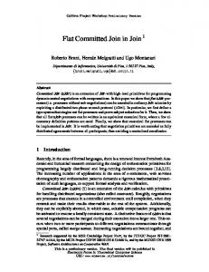
where Hg (k, i) = Hyper (|Dg|, j, k, i). For E[br (a)], i.e., a bad attribute value, we proceed similarly. For execution time, if we retrieve Dr o documents using Scan for the outer relation and send Qs queries for the inner relation, and retrieve Dr i documents, the execution time is:   Time(S,D1 ,D2 )=|Dr o |·(toR + toE )+|Dr i |· tiR + tiE +|Qs|·tiQ where toR and toE are the times to retrieve and process, respectively, a document for the outer relation, tiR and tiE are the times to retrieve and process, respectively, a document for the inner relation, and tiQ is the time to issue a query to the inner relation’s database. The value for |Dr o | is determined so that the resulting join execution meets the user requirements. E. Zig-Zag Join To analyze the ZGJN algorithm, we define a zig-zag graph consisting of two classes of nodes: attribute nodes (“a” nodes) and document nodes (“d” nodes), and two classes of edges: hit edges and generates edges. A hit edge A → D connects an a node to a d node, and denotes that a generated a hit on d, that is, d matches the query generated using a. A generates edge d → a connects a d node to an a node and denotes that processing d generated a. As an example, consider the zig-zag graph in Figure 8 for joining Mergers and Executives from Example 1 on the Company attribute. We begin with a seed query [“Microsoft”] for Mergers and issue it to the D2 database. This query hits a document d21 . Processing d21 generates tuples for Executives, which contain values Microsoft and AOL for Company. At this

Microsoft 12

Merck 22

IBM

Nike

11

Pepsico

For Pr q {grq |g(a), q}, we model querying as sampling over Hg (q) while drawing k · P (q) samples, and derive: g(a)    P rq {grq |g(a), q} = H g(a), i · Bg (i, grq )

11

23

Cisco AT&T

24

Fig. 8.

Sample zig-zag graph for Mergers   Executives.

stage, the total number of attributes generated for Executives is determined by the number of documents that matched the query [“Microsoft”]. Next, we issue the query [“AOL”] to D1 , which retrieves documents d11 and d12 . The total number of documents retrieved from D1 is determined by the number of attribute values generated for Executives in the previous step. Processing d11 for Mergers generates a new attribute value, AOL, which is used to generate new queries for D2 , and the process continues. The above example shows that the characteristics of a ZGJN execution are determined by the total number of attribute values and documents that could be reached following the edges on the zig-zag graph. Thus, the structure of the graph defines the execution time and the output quality for ZGJN. We study the interesting properties of a zig-zag graph using the theory of random graphs [15]. Specifically, we build on the singlerelation approach in [10] to model our join scenario, and use generating functions to describe the properties of a zig-zag graph. We begin by defining two generating functions, h0 (x), which describes the number of hits for a randomly chosen attribute value, and ga0 (x), which describes the number of attributes generated from a randomly chosen document.   h0 (x) = pak · xk , ga0 (x) = pdk · xk k

k

where pak is the probability that a randomly chosen attribute a matches k documents, and pdk is the probability that a randomly chosen document generates k attributes. To keep the model parameters manageable, we approximate the distribution for pak with the attribute frequency distribution used by our general analysis (Section V-B), as the two distributions tend to be similar. Specifically, we derive the probability that an attribute a matches k documents using the probability that a is extracted from k documents. Our goal, however, is to study the frequency distribution of an attribute or a document chosen by following a random edge. For this, we use the method in [15], [10] and define functions H(x) and Ga(x) that, respectively, describe the attribute and the document frequency chosen by following a random edge on the zig-zag graph. ga0  (x) h0  (x) H(x) = x  , Ga(x) = x ga0  (1) h0 (1) where h0  (x) is the first derivative of h0 (x) and ga0  (x) is the first derivative of ga0 (x). To distinguish between the relations,

2    we denote the functions using subindices: Hi (x) and Gai (x), |Dr i | · tiR + ·tiE + |Qsi | · tiQ Time(S, D1 , D2 ) = respectively, describe the attribute and the document frequency i=1 distributions for Ri (i = 1, 2). 1 2 We will now derive equations for the number of documents |Qs | and |Qs | are the minimum values required for the output E[|Dr 1 |] and E[|Dr 2 |] retrieved from D1 and D2 , respectively, quality to meet the user-specified quality requirements. To summarize, in this section we analyzed each join algoand the number of attribute values E[|Ar 1 |] and E[|Ar 2 |] rithm for the various choices of document retrieval strategies generated for relation R1 and R2 , respectively. For our analysis, and IE system configurations. Our analysis resulted in formulas we exploit three useful properties, Moments, Power, and for the join quality composition in terms of the number of Composition of generating functions (see [15], [10]). The documents retrieved for each relation or the number of keyword distribution of the total number |Dr 2 | of documents retrieved queries issued to a database. Conversely, this analysis can be from D2 using attributes from R1 can be described by the used to determine these input values for a given output quality. function Dr 2 (x) = H1 (x). Further, the distribution of the attribute values generated from a D2 document picked by VI. I NCORPORATING O UTPUT Q UALITY following a random edge is given by Ga2 (x). Using the INTO J OIN O PTIMIZATION Composition property, the distribution of the total number Our optimization approach applies the analysis from Secof attribute values generated from Dr 2 is given by the function tion V to our general goal of selecting a join execution strategy Ar 2 (x) = H1 (Ga2 (x)). for a given user-specified quality requirement. We now discuss The total number |Ar 2 | of R2 attribute values that will how we derive various parameters used in the analysis, and be used to derive the D2 documents is a random variable present our overall optimization approach. with its distribution described by Ar 2 (x). Furthermore, the distribution of the documents retrieved by an R2 attribute value Estimating Model Parameters: The analysis in Section V picked by following a random edge is described by H2 (x). relies on three classes of parameters, namely, the retrieval Once again, using the Composition property, we describe the strategy-specific parameters, the database-specific parameters, distribution of the total number of D2 documents retrieved and the join algorithm-specific parameters. The retrieval using Ar 2 attribute values using the generating function strategy-specific parameters are the precision p(qi ) of each Dr 1 (x) = Ar 2 (H2 (x)) = H1 (Ga2 (H2 (x))). To describe the query qi for AQG, or the classifier properties Ctp and Cfp for total number |Ar 1 | of R1 attribute values derived by processing FS; the database-specific parameters are |Dg|, |Db|, |Ag|, |Ab|, a Dr 1 document, we compose Dr 1 (x) and Ga1 (x), and define as well as the document and attribute frequency distributions, for each relation, and the values for |Agg|, |Agb|, |Abg|, and Ar 1 (x) = Dr 1 (Ga1 (x)) = H1 (Ga2 (H2 (Ga1 (x)))). |Abb|. Finally, the join-specific parameters are H(q) and P (q) Next, we generalize the above functions for Q1 queries sent for OIJN and ZGJN. Of these, the retrieval strategy-specific from R1 attribute values and using the Power property: parameters and the join algorithm-specific parameters can be |Q | |Q | easily estimated in a pre-execution, offline step [10]. On the Ar 2 (x) = [H1 (Ga2 (x))] 1 Dr 2 (x) = [H1 (x)] 1 , other hand, estimating the database-specific parameters is a Finally, we compute the expected values E[|Dr 2 |] after we more challenging task [12]. have issued Q1 queries using R1 attribute values. For this, we We estimate the parameters for each relation, separately, resort to the Moments property. using maximum likelihood estimation (MLE) based on the  approach described in [12]. Our MLE model relies on the d |Q | [H1 (x)] 1 E[|Dr 2 |] = analytical models in Section V, where we showed how to dx x=1  estimate the output given the database-specific parameters; d |Q | [H1 (Ga2 (x))] 1 E[|Ar 2 |] = to estimate parameters, we observe the output and infer the dx x=1 database-specific parameter values that are the most likely to generate the observed output. Due to space restrictions, we Similarly, we derive values for E[|Dr 1 |] and E[|Ar 1 |]. We derived the total number of attributes E[|Ar 1 |] and cannot present our estimation process in detail, but we provide E[|Ar 2 |] for the individual relations, but we are interested the basic intuition behind it. Please refer to [13] for details. While retrieving documents from database D, we observe in the total number of good and bad attribute occurrences some attributes and their frequencies in the retrieved documents. generated for each relation. For this, we split the number So, for an attribute ai obtained from Dr , we use s(ai ) to denote of attributes in a relation, using the fraction of good or bad the number of documents in Dr that generated ai . These values attribute occurrences in a relation. For instance, reveal information about the actual contents of the database. |Ag1 | Formally, we attempt to find the database specific parameters E[|gr 1 |] = E[|Ar 1 |] · |Ag1 | + |Ab1 | that maximize the likelihood function:  Given the analysis above, we compute the execution time of a P r{s(ai )|parameters} L(parameters) = zig-zag join that satisfies the user-specified quality requirements: i if we issue |Qsi | queries and retrieve |Dr i | documents for To find the set of parameter values that maximize L(parameters), we use the models from Section V to express relation Ri , i = 1, 2, the execution time is:

P r{s(a)|parameters} as a function of the database parameters. document frequency distributions tend to be power-law for Using these derivations, we search the space of parameters to our relations. find the values that maximize L. An important advantage Retrieval Strategies: For FS, we used a rule-based classifier of our estimation method is that it does not require any created using Ripper [4]. For AQG, we used QXtract [2], which verification method to determine whether an observed tuple relies on machine learning techniques to automatically learn is good or bad; the estimation methods derive a probabilistic queries that match documents with at least one tuple. In our split of the observed tuples, thereby carrying out the parameter case, we train QXtract to only match good documents, avoiding estimation process in a stand-alone fashion. We define a similar the bad and empty ones. likelihood function for the document frequencies. Using the estimated parameter values for each individual relation, we Tuple Verification: To verify whether a tuple is good or bad, we follow the template-based approach described in [11]. then numerically derive the join-specific parameters [13]. Additionally, we also use a web-based “gold” set from Putting It All Together: Our optimizer takes as input the user- www.thomsonreuters.com/. provided minimum number of good tuples τg and the maximum Join Task: We defined a variety of join tasks involving number of bad tuples τb , and picks an execution strategy to combinations of the three relations and the three databases. efficiently meet the desired quality level. The optimizer begins For our discussion, we will focus on the task of computing with an initial choice of execution strategy that uses IDJN and the join HQ   EX, with NYT96 and NYT95 as the hosting SC for each relation. As the initial strategy progresses, the databases for HQ and EX, respectively. optimizer derives the necessary parameters and determines a desirable execution strategy for τg and τb , while periodically Join Execution Strategies: To generate the join execution (e.g., every 100 documents) checking the robustness of the strategies for a task, we explore various candidates for individual relations and combine them using the three join new estimates using cross-validation [10], [12], [13]. A fundamental task in the optimization process is to identify algorithms of Section IV. For each relation, we generate singlethe Cartesian space to explore for a given quality requirement. relation strategies by using two values for minSim (i.e., 0.4 Exhaustively “plugging in,” for each database in our output qual- and 0.8) and combining each such configuration with the three ity model in Section V, all possible values for |Dr | (0, . . . , |D|) document retrieval strategies. or |Qs| (0, . . . , |Ag|+|Ab|) is inefficient, so instead we resort to Metrics: To compare the execution time of an execution plan a simple heuristic to minimize the sum of documents retrieved chosen by our optimizer against a candidate plan, we measure and processed (and hence the total execution time), conditioned the relative difference in time by normalizing the execution time on the product of the number of occurrences of good attribute of the candidate plan by that for the chosen plan. Specifically, values in each relation. Specifically, we aim to reduce the we note the relative difference as tc , where tc is the execution to difference between the number of documents retrieved for time for a candidate plan and to is the execution time for the each relation, since intuitively we are minimizing the sum of plan picked by the optimizer. two numbers, conditioned on their product. Thus, we select Accuracy of the Analytical Models: Our first goal was to the number of documents for each database to be as close verify the accuracy of our analysis in Section V. For this, we as possible. Conceptually, this heuristic follows a “square” assumed perfect knowledge of the various database-specific traversal of the Cartesian space D1 × D2 (see Section IV). parameters: we used the actual frequency distributions for each attribute along with the values for |Dg|, |Db|, and |De | for each VII. E XPERIMENTAL E VALUATION database. Given a join execution strategy, we first estimate the output quality of the join, i.e., E[|Tgood  |],  |] and E[|Tbad We now describe the experimental settings and results. using the appropriate analysis from Section V, while varying IE Systems: We trained Snowball [1] for three rela- values for the number of retrieved documents from the database, tions: ExecutivesCompany, CEO, HeadquartersComp− i.e., |Dr | and |Dr |. For each |Dr | and |Dr | value, we 1 2 1 2 any, Location, and MergersCompany, MergedWith, to measure the actual output quality for an execution strategy. which we refer as EX, HQ, and MG, respectively. For θ Figure 9 shows the actual and the estimated values for the (Section III-A), we picked minSim, a tuning parameter exposed good (Figure 9(a)) and the bad (Figure 9(b)) join tuples by Snowball, which is the similarity threshold for extraction generated using IDJN, Scan for both relations, and minSim patterns and the terms in the context of a candidate tuple. = 0.4. Similarly, Figure 10 shows the same results for OIJN Data Set: We used a collection of newspaper articles from when using Scan for the outer relation and minSim = 0.4 for The New York Times from 1995 (NYT95) and 1996 (NYT96), both relations. Then, Figure 11 compares the estimated and the and from The Wall Street Journal (WSJ). The NYT96 database actual values for ZGJN, for minSim = 0.4. We performed similar contains 135,438 documents, which we used to train the experiments for all other execution strategies. Additionally, extraction systems and the retrieval strategies. To evaluate we also examined the accuracy of the estimated number of the effectiveness of our approach, we used 49,527 documents documents for query-based join algorithms, i.e., for OIJN and from NYT96, 50,269 documents from NYT95, and 98,732 ZGJN. Figure 12 shows the expected and the actual number documents from WSJ. We verified that the attribute and of documents retrieved for varying number of queries issued

5

10

1

10

3

10

Estimated Actual 2

10

10 20 30 40 50 60 70 80 90 100

1

(a) (b) Fig. 9. Estimated and actual number of (a) good tuples and (b) bad tuples for HQ   EX, using IDJN with Scan and minSim = 0.4. 4

5

10

Number of tuples

Number of tuples

10

102

Estimated Actual 10 20 30 40 50 60 70 80 90 100

Percent of documents processed

10

10 20 30 40 50 60 70 80 90 100

104

103

102

Estimated Actual 10 20 30 40 50 60 70 80 90 100

Percent of documents processed

(a) (b) Fig. 10. Estimated and actual number of (a) good tuples and (b) bad tuples for HQ   EX, using OIJN with Scan and minSim = 0.4.

to each database, for ZGJN. Overall, our estimates confirm the accuracy of our analysis. Of these observations, we discuss the case for bad tuples for OIJN (Figure 10(b)) and ZGJN (Figure 11(b)), where our model overestimates the number of bad tuples. This overestimation can be traced to a few outlier cases. To gain insight into this, we compared the expected and the actual number of bad attribute occurrences. We observed four main cases where our estimated values were more than two orders of magnitude greater than the actual values. These attribute values frequently appeared in the database but were not extracted by the extraction system at the minSim setting used in our experiments. For instance, one such bad attribute occurrence, “CNN Center,” appears 895 and 2765 times in HQ and EX, respectively. When using OIJN and processing 50% of the database documents for the outer relation, our estimated frequencies of the bad occurrences of this value was 28.3 and 29.7 times, respectively; in reality, this attribute value was not extracted, thus resulting in an overestimate of 812 join tuples. This difference is further expanded for ZGJN due to a modeling choice: we assume that all queries used in ZGJN will match some documents and the execution will not stall. We can account for stalling by incorporating the reachability of a ZGJN execution based on the singlerelation analysis in [10]. Overall, while our estimates have non-negligible absolute errors, they identify the actual value trends appropriately, and hence allow our query optimization approach to pick desirable execution plans for a range of output quality requirements, as discussed next. Effectiveness of the Optimization Approach: After verifying our modeling, we studied the effectiveness of our optimization approach, which uses our models along with the parameter estimation process outlined in Section VI. Specifically, we examine whether the optimizer picks the fastest execution strategy for a given output quality requirement. For this, we

Estimated Actual 10 20 30 40 50 60 70 80 90 100

104 3

10

102 101

Percent of documents processed

Percent of documents processed

Percent of documents processed

103

2

10

Number of tuples

Estimated Actual

10

5

10

Estimated Actual 10 20 30 40 50 60 70 80 90 100

Percent of documents processed

(a) (b) Fig. 11. Estimated and actual number of (a) good tuples and (b) bad tuples for HQ   EX, using ZGJN with minSim = 0.4. 104

3

10

102

Estimated Actual 10 20 30 40 50 60 70 80 90 100

Percent of queries issued

Number of documents retrieved

2

10

4

Number of documents retrieved

103

103

Number of tuples

Number of tuples

Number of tuples

104

104

3

10

102

Estimated Actual 10 20 30 40 50 60 70 80 90 100

Percent of queries issued

(a) (b) Fig. 12. Estimated and actual number of documents retrieved for (a) HQ and (b) EX for HQ   EX, using ZGJN with minSim = 0.4.

provided the optimizer with the two thresholds, τg and τb . We report results for values of τg and τb for which the optimizer picked a satisfactory plan (i.e., the chosen execution matched the τg and τb quality requirements). In the future, we will systematically examine our optimizer’s ability to identify scenarios where no plan can match the quality requirements (e.g., as would likely be the case for, say, τb = 0), as well as those cases where our optimizer incorrectly predicts that no plan could match the quality requirements. To evaluate the choice of execution strategy for a specified τg and τb pair, we compare the execution time for the chosen plan S against that of the alternate executions plans that also meet the τg and τb requirements. Table II shows the results for HQ   EX, for varying τg and τb . For each τg and τb pair, we show the number of candidate plans that meet the τg and τb requirement. Furthermore, we show the number of candidate plans that result in faster executions than the plan chosen by our optimizer and the number of candidate plans that result in slower executions than the chosen plan. Finally, to highlight the difference between the associated execution times, we show the range of relative difference in time for both faster and slower execution plans. As shown in the table, our optimizer selects OIJN for low values of τg and τb , and progresses towards selecting IDJN coupled with AQG or FS, eventually picking IDJN coupled with SC for high values of τg and τb . For most cases, our optimizer selects an execution strategy that is the fastest strategy or close to the fastest strategy, as indicated by having either no candidates with faster executions than the chosen plan or a small number of such executions. For cases where the chosen plan is not the fastest option, the execution time of the faster candidates is close to the one of the chosen plan, as indicated by the relative difference values (e.g., a value of 1 indicates the execution times for both the candidate and the chosen plans were identical). An important observation is that the plans

Criteria τg 1 2 2 4 4 8 8 16 16 16 32 32 32 64 64 128 128 256 256 512 512 512 1024 1024

τb 20 30 50 20 40 40 80 50 80 160 84 160 320 320 640 640 1280 1280 2560 1024 2560 5120 5120 10240

Candidate plans 46 46 47 39 42 40 44 26 36 39 26 36 40 35 41 21 26 14 18 1 3 4 2 2

Chosen plan JN OIJN OIJN OIJN OIJN OIJN OIJN OIJN IDJN IDJN IDJN IDJN OIJN OIJN IDJN IDJN IDJN IDJN IDJN IDJN IDJN IDJN IDJN IDJN IDJN

θ1 0.4 0.8 0.8 0.4 0.4 0.8 0.8 0.4 0.4 0.4 0.4 0.8 0.8 0.8 0.8 0.4 0.4 0.4 0.4 0.8 0.8 0.4 0.8 0.8

θ2 0.4 0.4 0.4 0.4 0.4 0.4 0.4 0.4 0.4 0.4 0.4 0.4 0.4 0.4 0.4 0.4 0.4 0.4 0.4 0.8 0.4 0.4 0.4 0.4

X1 FS AQG AQG FS FS AQG AQG FS FS FS FS AQG AQG AQG AQG FS FS SC SC SC SC FS SC SC

X2 (OIJN) (OIJN) (OIJN) (OIJN) (OIJN) (OIJN) (OIJN) AQG AQG AQG AQG (OIJN) (OIJN) AQG AQG AQG AQG AQG AQG SC SC SC SC SC

# Faster plans

# Slower plans

5 10 11 3 3 3 4 3 3 1 1

36 32 33 29 37 33 38 21 30 34 22 35 39 34 40 20 25 13 17 2 3 -

Relative time range for faster plans min max 0.68 0.80 0.19 0.75 0.19 0.75 0.34 0.34 0.34 0.34 0.19 0.19 0.19 0.19 0.66 0.94 0.66 0.94 0.99 0.99 0.99 0.99

Relative time range for slower plans min max 1.20 27.48 1.78 11.91 1.78 11.91 1.59 35.76 1.59 35.76 1.15 22.20 1.15 22.20 1.22 11.62 1.10 11.62 1.10 11.62 1.26 13.30 1.55 20.62 1.55 20.62 1.50 27.16 1.50 27.16 1.19 9.41 1.19 9.41 1.18 2.89 1.01 2.89 1.02 1.15 1.46 1.69 -

TABLE II C HOICE OF EXECUTION STRATEGIES FOR DIFFERENT τg AND τb COMBINATIONS (S ECTION III-C), AND COMPARING THE EXECUTION TIME OF THE CHOSEN  EX. STRATEGY AGAINST THAT OF ALTERNATIVE EXECUTION STRATEGIES THAT ALSO MEET THE τg AND τb REQUIREMENTS , FOR HQ 

eliminated by the optimizer were an order of magnitude (10 to 35 times) slower than the chosen plans. An intriguing outcome of our experiments is that the choices for execution strategies do not involve ZGJN. Interestingly, for our test data set, ZGJN is not a superior choice of execution algorithm as compared to other algorithms. Intuitively, ZGJN does not specifically focus on filtering out any bad documents; therefore, ZGJN does not meet the quality requirements as closely as other query-based strategies that use IDJN or OIJN along with AQG or FS. Furthermore, the maximum number of tuples that can be extracted using ZGJN is limited, which makes it a poor choice for higher values of τg and τb . ZGJN would be a competing choice for scenarios involving databases that only provide query-based access (e.g., search engines or hiddenWeb databases) and also for cases where the generated queries match a relatively large number of good documents. Extending ZGJN to derive queries that focus on good documents remains interesting future work. VIII. C ONCLUSIONS We addressed the important problem of optimizing the execution of joins of relations extracted from natural language text. As a key contribution of our paper, we developed rigorous models to analyze the output quality of a variety of join execution strategies. We also showed how to use our models to build a join optimizer that attempts to minimize the time to execute a join while reaching user-specified result quality requirements. We demonstrated the effectiveness of our optimizer for this task with an extensive experimental evaluation over real-world data sets. We also established that the analytical models presented in this paper demonstrate a promising direction towards building fundamental blocks for processing joins involving information extraction systems.

IX. ACKNOWLEDGMENTS This material is based upon work supported by a generous gift from Microsoft Research, as well as by the National Science Foundation under Grants No. IIS-0811038, IIS0643846, and IIS-0347903. The third author gratefully acknowledges the support of an Alfred Sloan fellowship, an IBM Faculty Award, and grants from Yahoo and Microsoft.

R EFERENCES [1] E. Agichtein and L. Gravano. Snowball: Extracting relations from large plain-text collections. In DL, 2000. [2] E. Agichtein and L. Gravano. Querying text databases for efficient information extraction. In ICDE, 2003. [3] W. Cohen and A. McCallum. Information extraction from the World Wide Web (tutorial). In KDD, 2003. [4] W. W. Cohen. Learning trees and rules with set-valued features. In IAAI, 1996. [5] H. Cunningham, D. Maynard, K. Bontcheva, and V. Tablan. GATE: An architecture for development of robust HLT applications. In ACL, 2002. [6] A. Doan, R. Ramakrishnan, and S. Vaithyanathan. Managing information extraction (tutorial). In SIGMOD, 2003. [7] D. Ferrucci and A. Lally. UIMA: An architectural approach to unstructured information processing in the corporate research environment. In Natural Language Engineering, 2004. [8] R. Gupta and S. Sarawagi. Curating probabilistic databases from information extraction models. In VLDB, 2006. [9] P. Haas and J. Hellerstein. Ripple joins for online aggregation. In SIGMOD, 1999. [10] P. G. Ipeirotis, E. Agichtein, P. Jain, and L. Gravano. Towards a query optimizer for text-centric tasks. ACM Transactions on Database Systems, 32(4), Dec. 2007. [11] A. Jain, A. Doan, and L. Gravano. Optimizing SQL queries over text databases. In ICDE, 2008. [12] A. Jain and P. G. Ipeirotis. A quality-aware optimizer for information extraction. ACM Transactions on Database Systems, 2009. To appear. [13] A. Jain, P. G. Ipeirotis, A. Doan, and L. Gravano. Join optimization of information extraction output: Quality matters! Technical Report CeDER-08-04, New York University, 2008. [14] I. Mansuri and S. Sarawagi. A system for integrating unstructured data into relational databases. In ICDE, 2006. [15] M. E. J. Newman, S. H. Strogatz, and D. J. Watts. Random graphs with arbitrary degree distributions and their applications. Physical Review E, 64(2), Aug. 2001. [16] F. Reiss, S. Raghavan, R. Krishnamurthy, H. Zhu, and S. Vaithyanathan. An algebraic approach to rule-based information extraction. In ICDE, 2008. [17] W. Shen, A. Doan, J. Naughton, and R. Ramakrishnan. Declarative information extraction using Datalog with embedded extraction predicates. In VLDB, 2007.