Joint Angular Estimation and Wideband Spectrum

Faculty of Engineering Electrical Engineering Department

Port Said University

Joint Angular Estimation and Wideband Spectrum Sensing in Cognitive Radio Networks A thesis Submitted to the Electrical Engineering Department in partial fulfillment of the requirements for the degree of Master of Science in Electrical Engineering (Electronics and Communication) by

Samar Elsayed Elaraby Ahmed Hadou B.Sc., Electrical Engineering, Port Said University, 2011 Supervisors Professor Mohamed Abdel-Azim Mohamed Electronics and Communication Engineering Department Faculty of Engineering Mansoura University

Assistant Professor Heba Youssef Soliman Electrical Engineering Department Faculty of Engineering Port Said University

Assistant Professor Heba Mohamed Abdel-Atty Electrical Engineering Department Faculty of Engineering Port Said University

2017

Faculty of Engineering Electrical Engineering Department

Port Said University

Joint Angular Estimation and Wideband Spectrum Sensing in Cognitive Radio Networks A thesis Submitted to the Electrical Engineering Department in partial fulfillment of the requirements for the degree of Master of Science in Electrical Engineering (Electronics and Communication) by

Samar Elsayed Elaraby Ahmed Hadou B.Sc., Electrical Engineering, Port Said University, 2011 Approved by Professor Mustafa Mahmoud Abdel-Naby Diab Electronics and Communication Engineering Department Faculty of Engineering Tanta University

Professor Ahmed Shaaban Madian Samra Electronics and Communication Engineering Department Faculty of Engineering Mansoura University

Professor Mohamed Abdel-Azim Mohamed Electronics and Communication Engineering Department Faculty of Engineering Mansoura University

2017

Abstract Providing the dramatic increase in the number of radio devices due to the current advances in Internet of things (IoT), the shortage of frequency resources became a challenge to the new communication systems. To tackle this problem, cognitive radio (CR) has suggested to reutilize frequency bands left unoccupied by their licensed users raising the need to e↵ective estimation techniques that can detect these frequency bands. Additionally, if the spatial domain is investigated along with the spectral domain, a larger number of CRs can share the limited vacant bands simultaneously. In this thesis, the problem of estimating the special and spectral information of the existing users is considered for CR. The considered estimation problem should be handled blindly as CR should not have any prior information about the existing radio devices. Moreover, not only is the blindness the challenge of the considered problem, but also the need to instantaneously search a wideband spectrum, which needs high Nyquist rates. In order to overcome the latter issue, sub-Nyquist methods have been proposed in the literature. While these methods were capable to detect the desired parameters from reduced number of samples, they require a large number of relaxed analog-to-digital converters (ADCs) leading to increasing hardware complexity. In contrast to sub-Nyquist methods, which are carried out in the temporal domain, the proposed algorithms here are applied in the spatial domain of the employed array reducing the number of required samples at each array element to one. In addition, the proposed algorithms employ nonlinear Kalman filters (KFs), which are applied on a proposed spatial state space model, in two di↵erent scenarios; one of which estimates carrier frequencies and the corresponding direction of arrivals (DoA) of band-limited source signals, and the other one concerns with two-dimensional DoA (2DDoA). In each scenario, two di↵erent types of nonlinear KFs are implemented; the first is extended Kalman filter (EKF) and the other is unscented Kalman filter (UKF). Since nonlinear KFs are sub-optimal i

ABSTRACT estimators, their performance can be deteriorated by several factors such as filter tuning and initialization, the variance of the estimated variables, and the value of the inter-elements spacing in the employed array. Using simulations, the e↵ects of these factors on the filter performance are examined and discussed. Overall, relying on one time sample in the proposed algorithms eliminates the high-sampling-rate requirements, whereas exploiting the spatial domain in detecting the unknown parameters results in a gradual decline in the degrees of freedom.

ii

1

Dedication

To mum, the one who had been waiting for this moment for so long, and had dreamed of it more than anyone else including me. I wish you could be here among us today to see it come true. To all those people who severely su↵er from ignorance, oppression and all means of injustice all over the world. I wish spending our lives conducting research gave us an excuse for letting you down, and wish it made your world a more peaceful and reassured place. Samar

1

A dedication of what the signed person only shares of the rights; however, all the rights of the other contributors, i.e. the supervisors and university, are reserved.

iii

Acknowledgements The most important acknowledgment of gratitude I wish to express is to Allah for His blessings of giving me the patience and strength to complete this thesis, after all challenges and difficulties. I would like to express my deepest sense of gratitude towards my supervisor Dr. Heba Y. Soliman for her endless support, faithful guidance and unlimited patience. Her meticulous suggestions and inspiring discussions have lit up my way through the derivations of the proposed algorithms. She was also generous with her support providing me with all resources I needed. Her overwhelming support has exceeded this level and she starts to counsel me about my career beyond the thesis defense. Words cannot express how impressed really I am with her mentality and humility. She is a real role model. I would also like to express my sincere gratitude to my co-supervisor Dr. Heba M. Abdel-Atty for her wise advice, endless support, continuous encouragement and unlimited patience. I was always looking forward to her constructive criticism, which has taught me how to develop my research papers. I was totally impressed with her enthusiasm for research. She has kept on motivating and propelling me in situations in which I was exhausted, but she is always able to keep me on track. I have learnt many things from her that would boost my career, life and beyond. She is a true source of inspiration. Moreover, I would like to thank both of them, Dr. Soliman and Dr. Abdel-Atty, for the opportunities they have provided me with, putting full trust on me, and keeping on believing in me in spite of my weakness and deficiencies. I would like to thank Dr. Mohammed Abdel-Azim for his time, advice, enthusiasm and patience. His precious advice and suggestions v

ACKNOWLEDGEMENTS have helped to improve the quality of the research papers and thesis. It was a great honor to work under his supervision and learn from him. I would like to thank Dr. Ashraf Moukhtar for his session in Kalman filter last year. By that time, I had been looking for a solution for my thesis problem and had no clue yet. Then, his session was my “Eureka” moment. I hope his soul is blessed in heaven at this moment. I would like to express my deep appreciation to Egypt Scholars, a non-profit organization concerns with science and research, and their prestigious professors and researchers. With their help, I have learnt what it really means to be a researcher and how to conduct a scientific research successfully for the first time. I was inspired by their spirit, and they have made me develop a real passion for research. Finally, I would like to thank my parents and sisters for their belief in me, support, and faithful love and for bringing me up to be the person who I am today. Samar

vi

Contents Abstract

i

Dedication

iii

Acknowledgements

v

List of Abbreviations

xi

List of Symbols

xiii

List of Figures

xvi

List of Tables

xvii

List of Algorithms

xix

List of Publications

xxi

1 Introduction 1.1 Motivations . . . . . . . . . 1.2 Problem Statement . . . . . 1.3 Thesis Aims and Objectives 1.4 Thesis Contributions . . . . 1.5 Thesis Organization . . . . .

. . . . .

. . . . .

. . . . .

. . . . .

1 1 2 3 3 4

2 Spectrum Sensing for Cognitive Radio 2.1 Cognitive Radio . . . . . . . . . . . . . . . . . . . 2.2 Spectrum Sensing . . . . . . . . . . . . . . . . . . 2.2.1 Narrow-band Spectrum Sensing . . . . . . 2.2.2 Wideband Spectrum Sensing . . . . . . . . 2.2.3 Multi-antenna Assisted Spectrum Sensing 2.3 Joint Angular and Spectrum Sensing . . . . . . .

. . . . . .

. . . . . .

. . . . . .

7 7 9 11 14 17 22

vii

. . . . .

. . . . .

. . . . .

. . . . .

. . . . .

. . . . .

. . . . .

. . . . .

. . . . .

. . . . .

. . . . .

ACKNOWLEDGEMENTS 3 Fundamentals of Kalman Filters 3.1 Traditional Kalman Filters . . . . . . . . 3.2 Non-linear Kalman Filter . . . . . . . . . 3.2.1 Extended Kalman Filter (EKF) . 3.2.2 Unscented Kalman Filter (UKF) 3.2.3 EKF and UKF Performance . . . 4 Joint DoA and Carrier Frequency nique Using Nonlinear KFs 4.1 System Model . . . . . . . . . . . . 4.2 Proposed State Space Model . . . . 4.3 Proposed EKF-Based Approach . . 4.3.1 Prediction Step . . . . . . . 4.3.2 Updating Step . . . . . . . . 4.4 Proposed UKF-Based Approach . . 4.4.1 Selecting Sigma Points . . . 4.4.2 Prediction Step . . . . . . . 4.4.3 Updating Step . . . . . . . . 4.5 Results and Discussions . . . . . . 4.5.1 Experiment Setup . . . . . . 4.5.2 Simulation Results . . . . . 4.5.3 Comparative Study . . . . . 4.5.4 Performance Evaluation . . 4.6 Conclusions . . . . . . . . . . . . .

. . . . .

. . . . .

. . . . .

. . . . .

. . . . .

. . . . .

. . . . .

. . . . .

Estimation Tech. . . . . . . . . . . . . . .

. . . . . . . . . . . . . . .

. . . . . . . . . . . . . . .

. . . . . . . . . . . . . . .

. . . . . . . . . . . . . . .

. . . . . . . . . . . . . . .

. . . . . . . . . . . . . . .

. . . . . . . . . . . . . . .

. . . . . . . . . . . . . . .

. . . . . . . . . . . . . . .

. . . . . . . . . . . . . . .

5 Joint 2D-DoA and Carrier Frequency Estimation Technique Using Nonlinear KFs 5.1 System Model . . . . . . . . . . . . . . . . . . . . . . . 5.2 Proposed Spatial State Space Model . . . . . . . . . . 5.3 Proposed EKF-Based Approach . . . . . . . . . . . . . 5.4 Proposed UKF-Based Approach . . . . . . . . . . . . . 5.5 Results and Discussions . . . . . . . . . . . . . . . . . 5.5.1 Experiment Setup . . . . . . . . . . . . . . . . . 5.5.2 Simulation Results . . . . . . . . . . . . . . . . 5.5.3 Comparative Study . . . . . . . . . . . . . . . . 5.5.4 Performance Evaluation . . . . . . . . . . . . . 5.6 Conclusions . . . . . . . . . . . . . . . . . . . . . . . . viii

25 25 27 27 29 31

33 33 35 38 39 40 41 41 42 43 43 43 44 47 50 51

53 53 55 58 61 63 64 64 70 73 74

CONTENTS 6 Conclusions and Suggested Future Work 75 6.1 Conclusions . . . . . . . . . . . . . . . . . . . . . . . . 75 6.2 Suggested Future Work . . . . . . . . . . . . . . . . . . 76 Bibliography

79

ix

List of Abbreviations 2D-DoA ACS ADC BWB CaSCADE CCST CFD CS CR DoA DSA DSSS EBP ED EKF ESPRIT FFT FHSS FRESH FSA GLRT IoT KF LMS LO LPF M2M MCS MFD

Two-Dimensional Direction of Arrival Adaptive Cross-Self-coherent-restoral algorithm Analog-to-Digital Converter Bounded Worse Behavior CompreSsed CArrier And DoA Estimation Cyclic Correlation Significance Test Cyclostaionarity Feature Detector Compressive Sensing Cognitive Radio Direction of Arrival Dynamic Spectrum Access Direct Sequence Spread Spectrum Estimated Background Power Energy Detector Extended Kalman Filter Estimation of Signal Parameters via Rotational Invariance Technique Fast Fourier Transform Frequency Hopping Spread Spectrum FREquency SHift filter Fixed Spectrum Assignment Generalized Likelihood Ratio Test Internet of Things Kalman Filter Least Mean Square Local Oscillator Low Pass Filter Machine-to-Machine Multi-Coset Sampler Matched Fiter Detector xi

LIST OF ABBREVIATIONS MIMO MLE MME MUSIC MWC NBSS PAPR PARAFAC PU QoS RF RM2V RMSE RMT SCM SFET SNR SS SU SVD UKF ULA WBSS

Multiple Input Multiple Output Maximum Likelihood Estimation Maximum-Minimum Eigenvalue-based detector MUltiple SIgnal Classifier Modulated Wideband Converter Narrow-Band Spectrum Sensing Peak-to-Average Power Ratio PARAllel FACtor Primary User Quality of Service Radio Frequency Ratio of the Mean square to Variance Root Mean Square Error Random Matrix Theory Sample Covariance Matrix Separating Function Estimation Test Signal-to-Noise Ratio Spectrum Sensing Secondary User Singular Value Decomposition Unscented Kalman Filter Uniform Linear Array WideBand Spectrum Sensing

xii

List of Symbols

⌘xn ⌘yn ⌘zn ✓l l l 2 n a n 1 x n 1 x n|n 1

⇤ n|n 1

d f (.) h(.) ml rxn ryn rzn un wn w(c) w(m) xns ˆ0 x ˆ a0 x

Threshold value Noise signal in the nth element of x-array Noise signal in the nth element of y-array Noise signal in the nth element of z-array DoA of the lth source/ Elevation angle of the lth source Wavelength of the lth source Azimuth angle of the lth source Noise variance Prior sigma points Prior sigma points corresponding to the state variable Posterior sigma points Scaling parameter Posterior predicted measurements Inter-element spacing in L-shaped array Nonlinear process model Nonlinear measurement model The lth source signal Noise signal in the nth element of x-array Noise signal in the nth element of y-array Noise signal in the nth element of z-array Measurements noise signal Process noise signal Weights used to calculate the posterior covariance matrix Weights used to calculate the posterior estimate State variable in state n Initial estimate of the state variable Concatenation matrix of initial estimate of the state variable and measurements noise xiii

LIST OF SYMBOLS ˆn x ˆn 1 x ˆn x An Fn H H0 H1 Hn Kn L N P0 Pa0 Pn Pn Pn 1 P Q R ↵ Rxx (l) TED TGLRT TM M E TP AP R Xln Yl n Yn Zln (.)T max (.)

Updated posterior estimate of the state variable Prior estimate of the state variable Posterior estimate of the state variable Transition matrix in KF The Jacobian matrix of partial derivatives of f (.) Observation matrix that is constant over iterations The hypothesis that PU is absent The hypothesis that PU exists Observation matrix Filter gain Number of source signals Number of array elements in single ULA Initial covariance matrix of the state variable Initial covariance matrix of the state variable in UKF Updated posterior covariance matrix of the state variable Posterior covariance matrix of the state variable Prior covariance matrix of the state variable Measurements noise covariance matrix in UKF Process noise covariance matrix Measurements noise covariance matrix in KF and EKF The cyclic autocorrelation function of x(k) at lag l and cyclic frequency ↵ The hypothesis test for energy detector The hypothesis test for GLRT-based detector The hypothesis test for maximum-minimum eigenvaluebased detector The hypothesis test for PAPR-based detector The signal of the lth source received by the nth element of x-array The signal of the lth source received by the nth element of y-array Observed measurements The signal of the lth source received by the nth element of z-array Transpose matrix Maximization operator

xiv

List of Figures 2.1 2.2 2.3 2.4 2.5 2.6 2.7 2.8 2.9 2.10 2.11

DSA concept, quoted from [3] . . . . . . Cognitive cycle, quoted from [3] . . . . . Spectrum sensing modes, quoted from [3] Spectrum sensing techniques . . . . . . . Matched filter detector . . . . . . . . . . Energy detector . . . . . . . . . . . . . . Cyclostationay feature detector . . . . . Multi-joint detector, quoted from [4] . . Filter bank system, quoted from [4] . . . MCS system, quoted from [4] . . . . . . MWC front-end, quoted from [27] . . . .

. . . . . . . . . . .

8 8 10 11 12 13 13 15 15 16 17

3.1 3.2 3.3

EKF concept, quoted from [90] . . . . . . . . . . . . . UKF concept, quoted from [90] . . . . . . . . . . . . . Di↵erence between EKF and UKF with wide-spread state variable, quoted from [90] . . . . . . . . . . . . . Di↵erence between EKF and UKF with narrow-spread state variable, quoted from [90] . . . . . . . . . . . . .

28 29

L-shaped uniform array model . . . . . . . . . . . . . . Estimated parameters over iterations . . . . . . . . . . Joint estimated carrier frequency and DoA using EKF and UKF . . . . . . . . . . . . . . . . . . . . . . . . . RMSE in estimated parameters at di↵erent initial estimates . . . . . . . . . . . . . . . . . . . . . . . . . . . Estimated DoA and carrier frequencies at di↵erent interelement spacing . . . . . . . . . . . . . . . . . . . . . . Overall RMSE of the proposed algorithms and Kumar et al. [76] . . . . . . . . . . . . . . . . . . . . . . . . .

34 45

Two L-shaped uniform array model . . . . . . . . . . .

54

3.4 4.1 4.2 4.3 4.4 4.5 4.6 5.1

xv

. . . . . . . . . . .

. . . . . . . . . . .

. . . . . . . . . . .

. . . . . . . . . . .

. . . . . . . . . . .

. . . . . . . . . . .

. . . . . . . . . . .

32 32

46 47 48 51

LIST OF FIGURES 5.2 5.3 5.4

5.5 5.6 5.7

RMSE in the estimated azimuth, elevation and normalized wavelength . . . . . . . . . . . . . . . . . . . . . . Estimated carrier frequencies and their corresponding 2D-DoA . . . . . . . . . . . . . . . . . . . . . . . . . . RMSE in the estimated azimuth, elevation and normalized wavelength with initial estimates of 0.7 and di↵erent inter-element spacing . . . . . . . . . . . . . . . . . Estimated carrier frequencies and their corresponding 2D-DoA for di↵erent number of sources . . . . . . . . . RMSE in the estimated carrier frequencies and their corresponding 2D-DoA at di↵erent SNRs . . . . . . . . Overall RMSE of the proposed algorithms and Kumar et al. [85] . . . . . . . . . . . . . . . . . . . . . . . . .

xvi

65 66

67 69 70 74

List of Tables 4.1 4.2 5.1 5.2 5.3

Actual and estimated DoAs and normalized carrier frequencies of 6 di↵erent sources . . . . . . . . . . . . . . Comparison among the proposed algorithms and two other methods from the literature . . . . . . . . . . . . DoAs and normalized carrier frequencies of 12 di↵erent sources . . . . . . . . . . . . . . . . . . . . . . . . . . . Actual and estimated 2D-DoAs and normalized carrier frequencies of 12 di↵erent sources . . . . . . . . . . . . Comparison among the proposed approaches, Kumar et al. [85] and Kumar et al. [76] . . . . . . . . . . . . . .

xvii

44 49 64 65 72

List of Algorithms 3.1 3.2 3.3 5.1 5.2

KF algorithm . . . . . . . . . . EKF algorithm . . . . . . . . . UKF algorithm . . . . . . . . . EKF-based proposed algorithm UKF-based proposed algorithm

xix

. . . . .

. . . . .

. . . . .

. . . . .

. . . . .

. . . . .

. . . . .

. . . . .

. . . . .

. . . . .

. . . . .

. . . . .

. . . . .

26 28 30 59 62

List of Publications • S. Elaraby, H. Y. Soliman, H. M. Abdel-Atty, and M. A. Mohamed, “Joint 2D-DOA and carrier frequency estimation technique using nonlinear Kalman filters for cognitive radio,” IEEE Access, pp. 25097-25109, 2017. • S. Elaraby, H. Y. Soliman, H. M. Abdel-Atty, and M. A. Mohamed, “Joint angular and spectral estimation technique using nonlinear Kalman filters for cognitive radio,” AEU - International Journal of Electronics and Communications, vol. 83, pp. 359-365, Jan 2018.

xxi

Chapter 1 Introduction 1.1

Motivations

Radio frequency shortage has recently grabbed intensive attention as radio devices have increased tremendously. In the next few years, radio applications and devices are expected to exponentially grow due to the growth of Internet of things (IoT) and machine to machine (M2M) communication. In IoT, millions of edges and radio devices are going to communicate one another on radio frequencies, however the existing spectrum is limited and cannot be expanded to embrace the rising demand. On the other hand, the spectrum is exploited inefficiently, and many licensed bands are left unoccupied and rarely exploited by their licensed users. As a result, dynamic spectrum access (DSA) has been suggested to solve the frequency band shortage. Cognitive radio (CR), first introduced in 1999, is one of the technologies that implement DSA [1]. CR is a radio device that detects the frequency bands left unoccupied by their licensed users. Then, CRs can transmit on the unoccupied bands till their licensed users show up again. To accomplish this goal, the CRs are equipped with front-ends and algorithms that detect the unoccupied bands instantaneously. This way, the spectrum can be exploited wisely and many CRs can share the limited resources with the licensed users. In the literature, spectrum sensing, which is the process of detecting frequency bands left unoccupied by their licensed users, has drawn the attention of researchers in the last decade. Many proposals for spectrum sensing have been presented. The main target of spectrum sensing is to investigate a wideband spectrum instantaneously. This way, a larger number of CRs can share the detected vacant bands 1

Chapter 1

Introduction

instantaneously, which results in immense increase in the spectral capacity. More recently, to increase the number of CRs that can share unoccupied frequency bands in the same area at the same time, multiantenna techniques have been suggested to exploit the spatial domain as well. CRs have been employed to detect both the carrier frequency and direction of arrival (DoA) of the licensed users. As a result, the spectral and spatial domains can be exploited efficiently. However, the main obstacle facing the problem of investigating both the spectral and spatial domains is the need to sample a wideband spectrum at Nyquist rates. Nyquist rates require high-speed analog-to-digital converters (ADCs) and generate a large number of samples to be processed. Compressive sensing has been exploited to solve this problem by reducing sampling rates below Nyquist rates. However, the hardware complexity is still high in these proposals. This thesis is going to consider the joint carrier frequency and DoA estimation problem and introduce a novel technique to deal with its aforementioned obstacle.

1.2

Problem Statement

The problem being considered in this thesis is to estimate the spectral and spatial information of a number of band-limited and uncorrelated source signals. Two di↵erent scenarios are considered; the first is detecting carrier frequencies and the corresponding DoA of the source signals, and the other is detecting carrier frequencies and the corresponding two-dimensional direction of arrivals (2D-DoA). For this problem, the source signals are supposed to be band-limited signals spread over a wideband spectrum, which enforces the proposal to process wideband signals instantaneously to detect as many existing sources as possible. Thus, the proposal should have the ability to handle a wideband spectrum. In addition, the sources are expected to be anywhere in the same plane of the employed array in the first scenario, and anywhere around CR in the second one; in other words, the proposal should detect the sources from all directions. Another assumption made in the considered scenarios is that the source signals are only susceptible to additive Gaussian white noise, however any other channel implications are omitted. Moreover, the estimation problem should be executed blindly, as CRs should not have any prior information about the sources, their transmissions, or even their number. In short, the considered problem is to detect unknown number of 2

Introduction

Chapter 1

band-limited source signals that are spread over a wideband spectrum and located in any direction around the CR.

1.3

Thesis Aims and Objectives

The first aim of the thesis is to present a new method for detecting the carrier frequencies and the corresponding DoA of a number of bandlimited and uncorrelated source signals. In addition, the thesis also aims to examine the e↵ectiveness of nonlinear KFs in the considered problem, and study the advantages and disadvantages of this proposal compared to other methods in the literature. To achieve these aims, a number of objectives should be met. First, a review of the proposed methods for spectrum sensing and joint angular and spectrum sensing in the literature should be held. Then, the fundamentals of KF and its nonlinear types should be visited to deliberately study their sub-optimal performance and determine the factors that a↵ect the performance. After that, a proper array model should be selected for the considered problem before a spatial state space model, which KFs would follow in the estimation process, is proposed. Next, nonlinear KFs should be applied on the proposed state space model. To examine the e↵ectiveness of the proposed algorithms, simulations should be carried out over a large number of snapshots and at di↵erent circumstances. Detailed discussions and comparisons should be held to emphasize the performance of the proposed algorithms, examine the e↵ects of the factors that could negatively impact the filter performance, and compare between the di↵erent types of nonlinear KFs at di↵erent cases. Finally, comparisons with previous methods should be presented to determine what the proposals add to the literature, before conclusions and suggested future work are declared.

1.4

Thesis Contributions

In this thesis, a novel proposal for the joint carrier frequency and DoA estimation problem is presented based on nonlinear Kalman filters and an L-shaped array. The first contribution of the thesis is exploiting two types of nonlinear Kalman filters, extended Kalman filter (EKF) and unscented Kalman filter (UKF), in estimating both carrier frequencies and their corresponding DoAs. Kalman filter (KF) is widely exploited in estimation problems, however it has not been 3

Chapter 1

Introduction

exploited in the considered problem in this thesis before. Since EKF and UKF are sub-optimal estimators, they sustain degraded performance. To enhance their sub-optimal performance, the factors that a↵ect the performance are discussed. With simulations, it is proven that the filter performance can be enhanced under certain conditions on the filter tuning and initialization, the selected state variable to be estimated, and the inter-element spacing of the employed array. In order to reduce the hardware complexity associated with other proposals in the literature, the proposed algorithms exploit the spatial domain instead of the temporal domain by employing a traditional Lshaped array. Then, KF is applied in the spatial domain and predicts the unknown parameters from the relation between the signals at each array element and its successive, which means that the estimation process is carried out using one time shot only. This results in relaxing the hardware required in the Nyquist and sub-Nyquist proposals. This is considered as the second contribution of the thesis. The third contribution is that the proposed algorithms can be expanded to involve the second angle of 2D-DoA. The thesis first proposes nonlinear Kalman filter for estimating the carrier frequency and a single DoA of the licensed user using an L-shaped array. Then, the algorithm is extended to estimate the carrier frequency and the corresponding 2D-DoA, elevation and azimuth angles, of the licensed users using two L-shaped arrays. Exploiting two angles instead of a single angle increases the spatial capacity and exploits the resources more efficiently. As in this case, two di↵erent CRs can share the same frequency band and one angle while they di↵er in the other angle.

1.5

Thesis Organization

The thesis consists of 6 chapters. Chapter 2 and 3 concern with the background and the related work. In chapter 2, an overview of CR and spectrum sensing is provided. Then, a review of the related work in the literature is presented. In chapter 3, KF algorithms are reviewed, and the performance of EKF and UKF is studied. In chapter 4 and 5, the proposals are derived and discussed with appropriate simulations. Each proposal has been implemented by EKF and UKF separately. Chapter 4 presents the proposed algorithms for estimating the carrier frequency and the corresponding DoA of the licensed users. First, the state model is formulated for an L-shaped 4

Introduction

Chapter 1

array. Then, two di↵erent algorithms are derived using EKF and UKF. Simulation results are finally provided to show the performance of the proposed algorithms, and a comparison among the proposed work and two other proposals from the literature are presented. In chapter 5, the proposed algorithms for estimating the carrier frequencies and the corresponding 2D-DoA are presented. The state model is formulated this time for two connected L-shaped arrays. Then, two algorithms are presented using EKF and UKF. In the same manner, simulation results are finally stated to evaluate the performance of the proposed algorithms. Besides, a comparison between the proposed algorithms in this chapter and two other proposals from the literature are presented. Finally, chapter 6 declares thesis conclusions and suggested future work.

5

Chapter 2 Spectrum Sensing for Cognitive Radio In this chapter, a brief review of the proposed spectrum sensing (SS) techniques in the literature for cognitive radio are presented. First, a brief introduction to CR and its cognitive cycle are presented in section 2.1. Then, di↵erent SS techniques are reviewed in section 2.2. The review focuses on narrow-band spectrum sensing (NBSS), multiantenna assisted spectrum sensing and wideband spectrum sensing (WBSS) techniques. In section 2.3, a literature survey is presented to summarize the latest proposals for the joint carrier frequency and the corresponding DoA estimation problem, which is the problem considered in this thesis.

2.1

Cognitive Radio

As defined in [2], CR is an intelligent wireless communication system that is aware of its surrounding environment. This gained awareness is the gate to a new era where radio devices opportunistically access the spectrum without interfering each other. This process is known as DSA, in which the e↵orts have been exerted for a decade to overcome the recent spectrum scarcity and inefficient spectrum utilization. The main goal of CR is to allow unlicensed secondary users (SUs) to access the licensed bands when their primary users (PUs) are absent. The CR (used interchangeably with SU) should not threaten primary-user transmissions, so it has to withdraw from the frequency band as soon as a PU begins to transmit. This leads the CR to be aware of its surrounding environment. As a result, the CRs have to 7

Chapter 2

Spectrum Sensing for Cognitive Radio

be provided with efficient sensing techniques to detect PU existence instantaneously. When a PU is detected in one band, the CR should find another unoccupied band, called spectrum hole, to continue its transmission there. The whole process is illustrated in Figure 2.1. In order to achieve this goal, CR follows a sequence of steps, called cognitive cycle, shown in Figure 2.2. The steps of the cognitive cycle are SS, spectrum decision, spectrum sharing and spectrum mobility. The cooperation of the di↵erent processes in the cognitive cycle leads to accomplishing the main concept of CR [3]. In SS, the CRs

Figure 2.1: DSA concept, quoted from [3]

Figure 2.2: Cognitive cycle, quoted from [3] 8


Chapter 2

detect the existence of the PUs around them to be able to identify spectrum holes. This process should be executed continually even if the CR is transmitting over a spectrum hole. The reason is that PUs have the priority to use their licensed channels. Thus, the CRs should jump to another spectrum hole when a PU is present and begins to transmit. After identifying the available spectrum holes, the CR selects the appropriate spectrum hole depending on quality of service (QoS) requirements. The selection process is called spectrum decision. Since there are several CRs in the same area trying to access the same hole at the same time, their transmissions may be overlapped. Spectrum sharing provides the capability to share the spectrum resources among CRs and PUs as well and prevent any interference between all these transmissions. As aforementioned, CR should leave the band when a PU starts to transmit. However, the CR should continue its transmission over another spectrum hole. Spectrum mobility is responsible for giving the CR the ability to switch the frequency band smoothly and preventing its transmission from dropping. In this thesis, the main focus is on SS techniques which are going to be discussed in the next sections.

2.2

Spectrum Sensing

Basically, CR relies on SS to detect the unused spectrum holes which can be opportunistically assigned to SUs. Therefore, the CRs should own the ability to continuously sense the spectrum and transmit their signals during the absence of the PUs. In the literature, three di↵erent modes of SS have been developed for this purpose [3]. The first mode is primary receiver detection which aims to detect the PU receiver as shown in Figure 2.3a. Its main idea is that the CR detects the local oscillator (LO) leakage power emitted by the PU receiver during demodulation process. However, the leakage power is very weak, and the CR should be close enough to the PU receiver to recognize the leakage power. Thus, this mode is almost infeasible. The second mode is interference temperature management. In this mode, the CRs are allowed to transmit on the same band of the PU at the same time if they do not exceed a certain limit of interference, called an interference temperature limit. The problem is that the CRs cannot distinguish between the transmissions from the PUs and the other CRs. Then, it is hard to determine if they preserve the interference 9

Chapter 2


under the dedicated limit when the PU exists. The third and most popular mode is primary transmitter detection shown in Figure 2.3b. In this case, the CR detects the transmission of the PU to determine its existence.

(a) Primary receiver detection

(b) Primary transmitter detection

Figure 2.3: Spectrum sensing modes, quoted from [3] In primary transmitter detection, SS techniques can be classified into two main categories [4] as shown in Figure 2.4. The first category is NBSS in which the CR detects the existence of a single PU on a narrow-band channel. Many proposals have been presented in the literature, but the most popular techniques are matched filter detectors (MFD), energy detectors (ED) and cyclostationarity feature detectors (CFD). These techniques can determine whether a single PU exists on 10


Chapter 2

Spectrum Sensing (SS) Narrow-band Sensing (NBSS)

Wideband Sensing (WBSS)

Matched Filter MFD

Nyquist WBSS

Energy Detector ED

Sub-Nyquist WBSS

Cyclostationary feature detector CFD

Figure 2.4: Spectrum sensing techniques a dedicated narrow-band channel or not. However, SS should detect a large number of possible spectrum holes instantaneously. To achieve that goal, SS should be performed over a wideband spectrum. This increases the significance of the second category, WBSS.

2.2.1

Narrow-band Spectrum Sensing

The NBSS problem can be considered as a binary hypothesis test problem. The hypothesis model should distinguish between the existence of the PU and its absence. So, it can be defined as H0 : x(t) = n(t) H1 : x(t) = h(t) m(t) + n(t)

(2.1)

where H0 and H1 denote the PU absence and presence hypothesis respectively, and x(t) is the received signal. The signal m(t) represents the PU transmitted signal, n(t) is zero-mean additive white Gaussian noise, and h(t) represents the channel coefficient. NBSS techniques distinguish between the two hypotheses using a suitable threshold value. If the received signal exceeds a certain threshold, it means that the PU exists. However, if the received signal does not reach the threshold, it means that the received signal can be considered as noise signal and the PU does not exist. In the following, the most popular NBSS techniques are going to be discussed. 11

Chapter 2


1. Matched Filter Detectors (MFD) One of the popular detectors is MFD shown in Figure 2.5. MFD is a linear optimal filter used to maximize the signal-to-noise ratio (SNR) for coherent signal detection [5]. The optimal performance is gained from the fact that the impulse response of the filter is a reversed and shifted version of the signal to be detected. In MFD, the received signal is applied to a matched filter and then sampled at Nyquist rate. If the sampled value Y exceeds a threshold value , the detector declares PU existence. The main advantage of MFD is the fast sensing time [6]. However, it has two drawbacks. The first drawback is it needs prior information about the PU signals. The second one is the need to synchronize the CR and PU transmissions. x(t)

Rt

1 x(⌧ )m(T

y(t)

t + ⌧ )d⌧

Y

H1

Y ?

Decision H0 or H1

H0

Sampling at t = T

Matched Filter

Threshold Test

Figure 2.5: Matched filter detector

2. Energy Detectors (ED) In ED shown in Figure 2.6, the CR detects the presence of the PU based on the energy of the received signals. If the energy of the received signals exceeds a certain threshold value , a PU signal is detected. The threshold value is determined based on the noise variance of the channel. So, ED is highly susceptible to unknown or changing noise levels. The main advantages of this type of detectors are simplicity and that it does not require any prior information about PU signals. However, it takes larger time to sense the channel than matched filters as ED calculates the energy of the received signals over a long period of time [6]. Moreover, ED cannot distinguish between the PU signals and the other CR transmissions, which means that each CR is a↵ected by the transmission of the other CRs. Furthermore, ED cannot be applied on spread spectrum signals like direct sequence spread spectrum (DSSS) and frequency hopping spread spectrum (FHSS) signals [6]. These signals needs more sophisticated signal processing algorithms than the ED algorithm. Lastly, ED is susceptible to noise uncertainty. When SNR decreases under a certain level called SNR wall, energy detector cannot detect the PU signals reliably. 12

Spectrum Sensing for Cognitive Radio x(t)

⇣ ⌘2

Squarer

RT 0

Chapter 2 Decision H0 or H1

H1

dt

Integrator

Y ?

H0

Y

Threshold Test

Figure 2.6: Energy detector To overcome noise uncertainty, many proposals are presented to the literature. The first proposal is bounded worse behavior (BWB) model where the noise power is estimated into a bounded range and its upper bound replaces the noise power [7]-[10]. Another model, called estimated background power (EBP), has been proposed in [8], [11] and [12]. In EBP, an estimated noise power is employed to guarantee robustness against noise certainty. On the other hand, the authors in [13] have investigated the e↵ects of interferences of multiple PUs on ED. 3. Cyclostationay Feature Detectors (CFD) In a di↵erent manner, CFD, shown in Figure 2.7, exploits the fact that man-made signals exhibit periodicity in its statistics like mean and autocorrelation, in contrast to noise signals which are wide-sense stationary signals. Thus, for a signal x(k), the autocorrelation function at lag l and cyclic frequency ↵ may be expanded in the form of Fourier series [14], with the Fourier series coefficients being ↵ Rxx (l) = hx(k) x⇤ (k

l) e

j2⇡↵k

i

(2.2)

↵ where h.i operator represents time averaging. The term Rxx (l) is called the cyclic autocorrelation function at lag l and cyclic frequency ↵. However, for a signal that does not exhibit cyclostationarity at ↵ ↵, like additive noise, Rxx (l) = 0 8l. Therefore, cyclostationaritybased techniques can easily di↵erentiate the signals from noise. Not to mention, CFD can di↵erentiate among the PU signals and the other CR transmissions as both of them have non-zero cyclic autocorrelation

x(t)

Correlator

Average over T

Y

H1

Y ?

Decision H0 or H1

H0

Threshold Test

Figure 2.7: Cyclostationay feature detector 13

Chapter 2


function at di↵erent cyclic frequencies. Another obstacle of CFD is its higher complexity than other NBSS techniques.

2.2.2

Wideband Spectrum Sensing

The aforementioned NBSS techniques are inefficient approaches for CR. The CRs are supposed to sense a wide range of frequencies, i.e., up to a few Gigahertz, in short periods of time. So, they can quickly detect as many unoccupied spectral holes as possible to allow a large number of CRs to access the spectrum and transmit their signals. Thus, the spectral capacity would de tremendously enlarged. NBSS techniques are not able to attain this aim in spite of their promising performance. Then, new techniques, known as WBSS, are proposed to widely and instantaneously sense wide bands of the spectrum. As a result, WBSS techniques have gained immense interest in the last few years, and many proposals have been presented in the literature. The main challenge faces WBSS is the high sampling rate required to sample the wideband signals. According to Nyquist-Shannon theorem, the sampling rate should be twice the bandwidth of the signal to prevent aliasing. Then, WBSS needs high-speed ADCs, which are very expensive or even infeasible. It also leads to a large number of samples to be processed. As a result, new proposals have been introduced at sub-Nyquist sampling rates to reduce the complexity of these systems. In the following, a brief of WBSS proposals at both Nyquist and sub-Nyquist rates is presented. 1. Nyquist Wideband Spectrum Sensing In Nyquist WBSS, the proposals rely on a standard ADC which operates at Nyquist rates. To reduce the complexity of these techniques, they have been proposed depending on multi-channel systems to process the huge resultant samples. This, in turn, could reduce the time required to process all these samples. In [15], a multiband joint detector has been proposed. The wide band signal is sampled at high Nyquist sampling rate and then these samples are divided into parallel data using a serial-to-parallel conversion circuit. Fast Fourier transform (FFT) is then applied to convert the sampled wideband signal to the spectrum domain. The spectrum is then divided into multiband spectra and each band is investigated separately. The whole system is illustrated in Figure 2.8. In this proposal, the sampling rate increases 14


Chapter 2

Figure 2.8: Multi-joint detector, quoted from [4] with the increase of the bandwidth of the target spectrum and then it produces a larger number of samples. To relax the high sampling rate, a filter bank system has been proposed in [16] and [17]. The filter bank system, shown in Figure 2.9, is used to divide the wideband signal into narrow-band signals which are demodulated to a lower frequency. Each signal is then sampled separately at a low rate and investigated by conventional NBSS techniques. As shown in Figure 2.9, all the signals are processed in parallel to reduce processing time. Although the filter bank algorithm reduces the required Nyquist sampling rate, its implementation exploits a large number of RF components. 2. Sub-Nyquist Wideband Spectrum Sensing Since Nyquist WBSS techniques su↵er from high sampling rates and high implementation complexity, the attention of researchers has been drawn to sub-Nyquist techniques. In sub-Nyquist WBSS, the received signals are sampled at lower rates than the Nyquist rate. Compressive

Figure 2.9: Filter bank system, quoted from [4] 15

Chapter 2


sensing (CS) is the technique that brings this approach to reality. CS theory claims that signals can be recovered from fewer measurements than the Nyquist samples if the signals su↵er from sparsity in some domain. In the considered problem, the sparsity condition is fulfilled in the frequency domain where the spectrum is exploited inefficiently using the fixed spectrum assignment (FSA) policy. As a result, CS can be exploited in the sub-Nyquist WBSS techniques. This approach has been first introduced in [18]. The authors have reconstructed the wideband spectrum from low measurements using CS. After that, wavelet-based edge detection has been employed to detect the possible spectrum holes. To improve the robustness against noise uncertainty, the authors of [19] have proposed a cyclic feature detection-based compressive sensing algorithm. It reconstructs the 2D cyclic spectrum of wideband signals from compressed measurements. The spectrum holes can eventually be detected using energy detectors. In order to implement sub-Nyquist rates, di↵erent samplers have been proposed in the literature, such as multi-coset samplers (MCS) and modulated wideband converter (MWC). MCS, shown in Figure 2.10, divides the signals into uniform blocks, and then it retains some samples from each block that sustain the minimal rates and eradicates the other samples. The proposals of [20]-[22] have exploited MCS to sample the signals at the minimal rates, developed di↵erent reconstruction algorithms to restore the spectrum, and then applied any known sensing technique. In contrast, MWC exploits spread spectrum techniques [23]. MWC consists of an analog front-end with several channels as shown in Figure 2.11. The input signal is multiplied by a di↵erent periodic signal in each channel, and then the resultant is lowpass filtered (LPF) and sampled at sub-Nyquist rate. The authors in [23]-[26] have exploited this architecture in performing sub-Nyquist sampling and have proposed di↵erent methods to reconstruct the spec-

Figure 2.10: MCS system, quoted from [4] 16


Chapter 2

Figure 2.11: MWC front-end, quoted from [27] trum from the produced sub-Nyquist samples. Since the WBSS problem has no interest in the spectrum itself and it aims only to detect PU existence, some proposals have exploited the power spectrum instead. The power spectrum estimation of wide-sense stationary signals has been proposed in [28] using MCS. Furthermore, the proposal in [29] can reconstruct the power spectrum of wide-sense stationary signals using least squares algorithm by exploiting the cross-correlation between the di↵erent outputs of a modified MCS. In contrast to these methods that require sparsity in the power spectrum, the authors of [30] have developed a technique to reconstruct the power spectrum without any sparsity constraints. Although the sparsity in the frequency domain is the solution for today challenge, it would be the challenge tomorrow. The sparsity in the frequency domain is caused by the inefficient spectrum utilization. Since CR aims to exploit empty frequency bands, the spectrum will be crowded and sparsity will be diminished. As a result, the performance of the current proposals will be degraded. Thus, other domains should be investigated.

2.2.3

Multi-antenna Assisted Spectrum Sensing

One issue encountered with all SS methods is the e↵ect of channel fading between the PU and CR. There is a decrease in the probability of detection whenever the channel is in a deep fade. This can be alleviated by exploiting spatial diversity either through the use of cooperative spectrum sensing [31] or the use of multiple antennas in single receivers. As a result, SS algorithms exploiting multiple anten17

Chapter 2


nas have received considerable interest in the literature [32]. In the same manner of that used in NBSS, multi-antenna assisted spectrum sensing follows a similar hypothesis model to the one described in Equation 2.1. The new model can be defined for an Nelement multi-antenna as H0 : x(k) = n(k) H1 : x(k) = h(k) m(k) + n(k)

(2.3)

where x(k) and n(k) 2 CN represent respectively the received signal and noise signal at the multi-antenna. The matrix h(k) represents the channel coefficients while m(k) is the PU transmitted signals. Accordingly, the following SS techniques aim to solve this problem by finding a threshold value which di↵erentiates between the two hypotheses. 1. Spatial Energy Detectors The simplest and more straightforward way to use energy detector with multi-antenna system is to average the signal power at all antennas and over all time instances [32]. Then, the ED hypothesis test TED becomes N K X X1 H1 TED = |xi (k)|2 ? (2.4) i=1 k=0

H0

where K is the number of snapshots used to average the power and is a threshold value. A di↵erent perspectives has been considered in [33] where ED is applied only to the highest-SNR signal among the several received signals at di↵erent antenna elements. The performance of these approaches is evaluated and They attain enhanced results over single-antenna-based ED. The authors in [34] have proposed a new way to optimally combine the received signals in time and space to maximize the SNR. To overcome the need to prior information of the PU, they have also proposed a blindly combined ED. The advantages and disadvantages of spatial ED are similar to conventional ED. However, spatial energy detector gives higher performance. Moreover, multi-antenna can be exploited in a full-duplex sensing technique where the CR can transmit its signals and detect the PUs at the same time. For this goal, the authors in [35] have proposed using a portion of array elements in transmitting while the other elements are detecting the PUs. 18


Chapter 2

2. Cyclostationarity Feature Detectors The main goal of employing multi-antenna in CFD is to enhance the cyclostationary features of the signal of interest. In [36], the authors have benefited from adaptive cyclostationarity beamforming techniques that have the ability to extract any number of signals from cochannel interference using their cyclic frequency. So, the authors have exploited a beamforming techninque, called adaptive cross-selfcoherent-restoral (ACS) algorithm, to propose an efficient SS method with a↵ordable complexity. ACS algorithm, proposed in [37], is an adaptive beamforming algorithm which aims to maximize the strength of the spectral cross-correlation coefficient between an array output signal and a reference signal. In [38], the authors have decided to improve the cyclostationary features of the signal of interest by combining a blind frequency shift (FRESH) filter with a modified ACS algorithm to pool the benefits o↵ered by both two approaches. The objective of the proposed algorithm is to minimize the di↵erence between the filtered and the reference signal instead of maximizing their cross correlation as in [37]. Besides, a lower complex adaptive beamforming technique, based on the least mean square (LMS), has been proposed to replace ACS in [38]. Moreover, the authors in [39] have proposed another CFD based on the cyclic correlation significance test (CCST). This method has been found more robust to noise uncertainty as the threshold does not depend on SNR. 3. PAPR-Based Detectors Since ED is inefficient in the low SNR conditions, peak to average power ratio (PAPR) based detector has been proposed. This approach, discussed in [40], exploits the ratio between the maximum received power and the average power of the recieved signal. The authors have chosen to power their beamformer by conventional beamforming [41]. The maximum received power can be obtained by steering the beam toward the desired DoA. Consider that the power of noise and the signal are n2 and s2 respectively. The maximum power is found to be N 2 s2 + N n2 at the existence of the PU, and becomes N n2 at its absence. Then, PAPR hypothesis test TP AP R has been proposed as TP AP R =

max P (✓)

H1

E[P (✓)]

H0

✓

19

=1

(2.5)

Chapter 2


where P (✓) is the power of the incident signal from direction ✓. Although PAPR approach outperforms ED under all SNR conditions, PAPR is more complex than ED. Thus, a hybrid system based on the channel state has been investigated in [42]. The proposed algorithm chooses ED at good channel conditions and switches to PAPR for bad channel conditions. Another detector has been proposed in [43]. This proposal depends on the ratio of the mean square to variance (RM2V) of the samples at the array element outputs. From simulations in [43], it has been proven that RM2V algorithm outperforms the performance of ED.

4. MME-Based Detectors Maximum-minimum eigenvalue (MME) algorithm depends on eigenvalues of the correlation matrix of the received signal, which has been derived in [44]. The hypothesis test of MME-based detector TM M E has been defined as the ratio between the maximum and minimum eigenvalues of the correlation matrix and can be expressed as TM M E =

max

H1

?

(2.6)

min H0

where max and min are the maximum and minimum eigenvalues respectively. This ratio can be quantized by random matrix theories (RMT), and hence a threshold can be calculated without the need of prior information about the signal. In [44]-[47], di↵erent proposals have been proposed for evaluating the threshold for MME-based detector. The results have proven a higher performance of MME-based detector than the performance of ED. Thus, MME overcomes the noise uncertainty difficulty while keeps the advantages of ED. Recently, the authors in [48] have proposed a new method that exploits the whole eigenvalues of the sample covariance matrix instead of partial information, like the maximum and minimum values. The authors in [49] and [50] have considered this problem from another perspective using the second order moments of the eigenvalues of the sample covariance matrix (SCM). They have exploited separating function estimation test (SFET) framework [51] to establish such detectors. 20


Chapter 2

5. GLRT-Based Dectectors Many authors have proposed multi-antenna assisted SS techniques with the using of multiple antenna based on generalized likelihood ratio test (GLRT), which is described in [52]. GLRT is suitable for composite hypothesis test where some or all of the statistics of the signals and noise are unknown. GLRT-based detector [53], first estimates the unknown statistics of noise, the channel and primary signals by using maximum likelihood estimation (MLE) b0 = arg max p(x|H0 , ⇥0 ) ⇥ ⇥0

b1 = arg max p(x|H1 , ⇥1 ) ⇥

(2.7)

⇥1

where ⇥0 and ⇥1 are sets of the unknown parameters under H0 and H1 , respectively. Then, the GLRT hypothesis test TGLR is performed TGLR =

b 1 ) H1 p(x|H1 , ⇥ ? b 0 ) H0 p(x|H0 , ⇥

(2.8)

In [32] and [54], the authors have proposed blind SS approaches that detect only the PU Gaussian-distributed signals. The results have shown that the proposed approaches exhibit a better performance than the other conventional techniques with single antennas. In [55] and [56], GLRT-based detectors have been proposed for detecting spatial rank-1 signals, however, in practical scenarios the spatial rank of the received signals should be larger than one. Thus, GLRT-based detectors for spatial rank-p signals have been introduced in [57] and [58]. In modern communication, PU transmitters are more likely to employ multi-antenna, and hence the authors in [59] have proposed a blind GLRT-based detector for detecting the PUs employing multi-antenna. Other di↵erent scenarios have been considered in the literature. The authors in [60] have brought robustness to the GLRT-based detectors in the case of high dimensionality and small sample size. They have proposed a modified GLRT-based detector by exploiting spatiotemporal covariance matrix. Simulations have shown advantages over existing detectors. Since most of the proposals in the literature assume that noise signals in di↵erent array elements are spatially uncorrelated signals, most recent proposals have focused on correlated noise signals. The authors in [61] have handled the case where noise signals are correlated due to mutual coupling between array elements, and 21

Chapter 2


the authors of [62] have considered GLRT-based detectors in colored noise in MIMO environments. Moreover, other di↵erent environments and situations have been handled recently. For example, fading environments and the full-duplex mode have been also considered in [63] and [64] respectively. 6. Bayesian-Based Detectors As an alternative approach to GLRT, bayesian-based approach has been introduced in [65] to detect the presence of the PU with a prior information about noise and the channel statistics. In [66] and [67], the authors have proposed another bayesian detector, which exploits prior information obtained from the past sensing frame. Since bayesian detectors rely on prior information, their performance outperforms GLRT-based detectors.

2.3

Joint Angular and Spectrum Sensing

The sparsity of the frequency domain is not guaranteed after employing CR and hence WBSS techniques may deteriorate with time. Thus, other domains are preferred to be considered and exploited. One of these domains is angular frequency domain which represents the power spectrum in respect of both frequency and DoA. Many proposals have been presented in the literature to jointly detect both carrier frequency and the corresponding DoA of the PU. Two perspectives have been considered. The first one is to detect single DoA and carrier frequency. The other one is detecting carrier frequency with two angles: azimuth and elevation. The problem of jointly estimating carrier frequencies and their corresponding DoAs has been addressed in [68]-[70] which assume that the signal is sampled at Nyquist sampling rate. However, the CR has to sense a wideband spectrum to increase the chance of detecting unoccupied bands, leading to high Nyquist sampling rates. High sampling rates, in turn, require high-speed ADCs and generate a large number of samples to be processed. Since Nquist-based proposals had been considered impractical because of the hardware complexity, signal processing community looked for new techniques that operate at sub-Nyquist sampling. Recently, sub-Nyquist rates have been considered for jointly estimating carrier frequencies and their corresponding DoAs problems. 22


Chapter 2

In [71], the authors have proposed a new architecture in which each array element is followed by two paths, a direct path and a delayed path. Each path is then followed by an ADC that operates at subNyquit rate. The authors have then proposed an algorithm that relies on ESPRIT algorithm [72] to detect carrier frequencies and MUSIC algorithm [73] to refine the estimated carrier frequencies and detect their corresponding DoAs. Finally, the spectrum has been blindly reconstructed. However, their algorithm has failed to pair the two estimated parameters with each other while using a uniform linear array (ULA). They instead have relied on uniform circular array. The authors in [74] have modified the architecture to achieve the required pairing of carrier frequencies with their corresponding DoAs while employing a ULA. The modified architecture has all the delayed paths connected after the first element of the ULA only. Another approach has been proposed in [75] to refine the estimated carrier frequencies and their corresponding DoAs in the presence of noise using a proposed 2D-iterative grid refinement. The main disadvantage of both two proposals in [71] and [74] is that their degrees of freedom are limited to the number of elements in the employing array. To increase degrees of freedom, the authors in [76] have employed a 2D nested array instead of a dense ULA. Because of its sparse dimensions, the degrees of freedom have increased leading to detecting a number of source signals larger than the number of array elements. In [77], CS has been proposed for reconstructing a sparse spectrum from sub-Nyquist rate samples and then detect carrier frequencies and DoAs using an L-shaped uniform array. Sub-Nyquist sampling has been implemented using a single channel employing an MWC. In contrast, proposal in [78] has employed several MWC samplers at the output of each array element leading to increasing the degrees of freedom. An alternative sub-Nyquist sampling and signal reconstruction depending on compressed carrier and DoA Estimation (CaSCADE) have been proposed in [79]. Since spectrum reconstruction is not required at this type of problems, the authors in [80] have reconstructed 2D power spectrum of a wide-sense stationary signal instead of the spectrum of the signal itself. This leads to overcoming spectrum sparsity constraints required in CS problems. The authors have proposed an MCS for compressing temporal measurements at sub-Nyquist rate. In a dual manner, a minimum redundancy linear array [81] has been employed to compress spatial measurements as well, leading to in23

Chapter 2


creasing the degrees of freedom. Furthermore, a more efficient scenario has addressed the idea of investigating 2D-DoA instead of a single DoA, which represents a single direction around CR. Then, the CR can share the same carrier frequency and azimuth angle with a licensed user, but they can di↵er in the elevation angle. This, in turn, increases the spatial capacity. The problem of jointly estimating 2D-DoA and carrier frequencies of PUs has been discussed in the literature. ESPRIT algorithm is widely applied on this problem. In [82], the authors have relied on ESPRIT algorithm to detect carrier frequencies from sub-Nquist samples of the source signals that impinge on a uniform circular array. Then, 2DDoA can be estimated. The authors in [83] have also implemented ESPRIT algorithm to estimate 2D-DoA using an L-shaped uniform array. However, carrier frequencies have been estimated by singular value decomposition technique (SVD). In [84], ESPRIT algorithm has been extended to estimate both carrier frequencies and 2D-DoA. In [85], another ESPRIT-based algorithm has been proposed for estimating the carrier frequencies and their corresponding 2D-DoA of multiband signals from the outputs of a uniform rectangular array (URA). Moreover, The PARAFAC analysis has been proposed for frequency and 2D-DoA estimation with a conformal array in [86] and [87]. In [88], the authors have proposed iterative least square methods to the joint frequency and 2D-DoA estimation problem. In this thesis, a novel technique is proposed for solving the joint carrier frequency and DoAs estimation problem using nonlinear Kalman filters. Estimating carrier frequencies is carried out over a wideband spectrum and the two perspectives of estimating DoAs are considered.

24

Chapter 3 Fundamentals of Kalman Filters In this chapter, a review of the fundamentals of KF is presented and followed by a brief description of its two popular nonlinear types. In section 3.1, the fundamentals of tradition linear KF is presented. Section 3.2 presents a review of EKF and UKF algorithms respectively and discusses their performance.

3.1

Traditional Kalman Filters

Kalman filter is a recursive algorithm that optimally estimates unknown state variables from state space models based on noisy measurements [89]. First, KF algorithm predicts the posterior estimate of the state variable from the previous estimate. Then, predictions are adjusted according to observed measurements. The two steps are repeated till the filter converges to the true estimate of the state variable. KF is considered as an optimal algorithm as it depends on linear state space model. A linear state space model can be generally described as a combination of process space model and measurement space model as follows x n = An x n 1 + wn Y n = H n x n + un

(3.1)

where xn and xn 1 denote the posterior and prior states respectively. The matrices An and Hn represent transition matrix and observation matrix respectively. Both of them can either vary over time or remain 25

Chapter 3

Fundamentals of Kalman Filter

constant. The matrix Yn represents observed measurements. However, wn and un respectively denote process noise and measurements noise signals, which are Gaussian distributed with zero mean and covariance matrix of Q and R respectively. Process noise covariance matrix Q represents uncertainty in process space model. However, measurements noise covariance matrix R represents uncertainty in observed measurements. While KF estimates the state variable, it can estimate unknown parameters as well. As a result, it is used intensively in estimation problems where the unknown parameters are concatenated to the state variable. Then, it can be estimated with it through iterations. The recursive algorithm, described in [89] and illustrated in Algorithm 3.1, consists of two steps: prediction step and updating step. ˆ n is In prediction step, the posterior estimate of the state variable x ˆ n 1 , and the predicted from the prior estimate of the state variable x posterior covariance matrix Pn of the state variable is also predicted from its prior version Pn 1 . The covariance matrix Pn reflects uncertainty of the current estimates, and it should decrease through iterations while the estimates approach the true values of the state variable. In updating step, the posterior estimates and covariance matrix are adjusted following the observed measurements Yn . Since KF is an optimal estimator, it succeeds to converge to the true values after several iterations of prediction and updating for any Algorithm 3.1 KF algorithm 0: loop: Prediction Step: ˆ n = An x ˆn x

1

Pn = An Pn

1

ATn + Q

Updating Step: Kn = Pn HTn (R + Hn Pn HTn ) ˆn = x ˆ n + Kn (Yn Hn x ˆn ) x Pn = Pn K n H n Pn if convergence: break loop 26

1


Chapter 3

filter initialization values. However, if KF is initialized with estimates values that are far away from the true values, it may need more iterations to converge. In contrast, nonlinear KFs have sub-optimal performance, which leads the filters to converge to local minima instead of the global minimum if the filters are not initialized properly.

3.2

Non-linear Kalman Filter

In many estimation problems, the state space model may have a nonlinear process model and/or a nonlinear measurement model. The nonlinear state space model has the form of [89] xn = f (xn 1 ) + wn Yn = h(xn ) + un

(3.2)

where f (.) and h(.) represent nonlinearity in the process and measurement models respectively. For nonlinear state space models, traditional KF fails to converge to the true values, and modifications to KF are required resulting in sub-optimal performance. Two of the renowned nonlinear KFs are EKF and UKF, which are going to be discussed in the following.

3.2.1

Extended Kalman Filter (EKF)

In EKF, detailed in [89], nonlinear models are linearized about the estimated trajectory. It relies on Taylor series to execute linearization and the resultant is approximated to the first order derivatives. As a result, linearization process leads to deviation in the filter output as shown in Figure 3.1 (see the di↵erence between the red and blue Gaussian distributions). In order to estimate the state variable, the filter follows the same iterative steps of traditional KF. In prediction step, the posterior estimates and covariance matrix are predicted using the Jacobian matrix Fn of the process model, which represent the linearized version of the process space model. In updating step, the measurement space model is also linearized to acquire the observation matrix Hn , and then the posterior estimates and covariance matrix are adjusted based on observed measurements. The detailed description of these steps is shown in Algorithm 3.2 as quoted from [89]. In comparison to KF, EKF has a deteriorated performance. Linearization process results in significant errors in the estimated state 27

Chapter 3


Figure 3.1: EKF concept, quoted from [90]

Algorithm 3.2 EKF algorithm 0: loop: Prediction Step: @f (xn 1 ) @xn 1 ˆ n = f (ˆ x xn 1 ) Fn =

xn

xn 1 1 =ˆ

Pn = Fn Pn 1 FTn + Q Updating Step: @Yn @xn xn =ˆxn Kn = Pn HTn (R + Hn Pn HTn ) ˆn = x ˆ n + Kn (Yn Hn x ˆn ) x Pn = Pn K n H n Pn Hn =

if convergence: break loop 28

1


Chapter 3

variables and these errors are accumulated through iterations. On the other hand, the filter updates the estimated state variable each iteration based on noisy measurements. This, in turn, leads the estimated trajectory to follow the noisy measurements. As a result, the filter may converge to erroneous values or even completely diverge. To enhance the performance of EKF, the filter should be tuned and initialized properly. Tuning the filter means to choose a proper estimate for Q and R matrices to wisely build confidence in both process and measurement models respectively.

3.2.2

Unscented Kalman Filter (UKF)

In UKF, proposed in [91], Gaussian distributed state variable is captured by a minimal set of sample points, called sigma points. These points are actually capturing both the mean and variance of the state variable. After sigma points are propagated through the nonlinear system, their outputs can be used to perfectly recover the estimated Gaussian state variable as shown in Figure 3.2. UKF is found to be accurate to the third order derivatives, which means that it has a better performance than the performance of EKF.

Figure 3.2: UKF concept, quoted from [90] 29

Chapter 3


The main steps of UKF algorithm is presented in Algorithm 3.3 quoted frpm [91]. In each iteration, a set of sigma points an 1 is ˆ an 1 , a conselected to capture the statistics of the prior estimates x ˆ n 1 and the estimates catenation of the estimates of the state variable x of process noise. The number of selected sigma points is 2M + 1 for xn 2 RM . The sigma points are then propagated through the model resulting in the posterior sigma points an|n 1 . In prediction step, the Algorithm 3.3 UKF algorithm 0: loop: Selecting Sigma Points: a 0,n 1

a i,n 1

ˆ an 1 x

=

a i,n 1

ˆ an =x

+

⇣p

Prediction Step:

1

⌘

(6L + ⇤)Pn

1

(6L + ⇤)Pn

1

x i,n|n 1

x i,n 1 )

⇣p

1

ˆ an =x

ˆn = x

12L X

= f( (m)

wi

⌘i i

, i = 1, 2 . . . M , i = M + 1, . . . 2M

x i,n|n 1

i=0

Pn =

12L X

(c)

wi

i=0

⇣

x i,n|n 1

ˆn x

⌘⇣

x i,n|n 1

ˆn x

⌘T

Updating Step: i,n|n 1

x i,n|n 1 ,

= h(

ˆn = y

12L X

n i,n|n 1 )

(m)

wi

i,n|n 1

i=0

Pyñ yñ =

12L X

(c)

wi

i=0

Pxñ yñ =

12L X i=0

(c)

wi

⇣ ⇣

i,n|n 1

ˆn y

x i,n|n 1

ˆn x

Kn = Pxñ yñ Pyñ1yñ

⌘⇣

⌘⇣

ˆn = x ˆ n + Kn (Yn x

i,n|n 1

ˆn y

i,n|n 1

ˆn y

ˆn ) y

Kn Pyñ yñ KTn

Pn = Pn if convergence: break loop

30

⌘T

⌘T


Chapter 3

posterior estimates and covariance matrix of the state variable are evaluated as weighted mean and covariance matrix of the posterior sigma points corresponding to state variable only xn 1 . The weights used in the evaluation of the recovered mean and covariance w(m) and w(c) are presented in [91]. In updating step, the posterior estimates are adjusted depending on observed measurements. The whole steps are presented in details in Algorithm 3.3. Through iterations, the filter tends to converge to the true values of the state variable. UKF needs to be properly tuned and initialized to enhance the filter convergence.

3.2.3

EKF and UKF Performance

Figures 3.1 and 3.2 show the di↵erence in performance between EKF and UKF. UKF has a better performance since it is accurate to the third order derivatives, whereas EKF is accurate to the first order derivatives. However, both of them are sub-optimal filters and have a lower performance than the performance of traditional KF. The performance of both EKF and UKF can be enhanced or deteriorated depending on the state space model and the state variable. Under some cases, they can approach the performance of traditional KF. Figure 3.3 shows the case of a state variable with a high variance relative to the region in which linearization is accurate. Both two filters show a deteriorated performance compared to their performance in Figures 3.1 and 3.2. However, UKF still has a better performance than EKF. On the other hand, Figure 3.4 shows the opposite case, a case of a state variable with a small variance relative to the region in which linearization is accurate. In this case, both EKF and UKF outperforms their ordinary performance and approaches the performance of traditional KF (the blue Gaussian distribution). The reason is that the state variable with small variance tends to operate in a small region where the model is relatively linear, and then the linearization errors diminish. In contrast, the state variable with high variance operates over a wide region which is susceptible to nonlinearity and then there are high linearization errors. This criteria is exploited in the proposed algorithms in the next two chapters by choosing a state variable with small variance relative to the formulated model to acquire a higher performance. Even though the proposed models in this thesis cannot be visualized, this advantage is proven with simulations.

31

Chapter 3


Figure 3.3: Di↵erence between EKF and UKF with wide-spread state variable, quoted from [90]

Figure 3.4: Di↵erence between EKF and UKF with narrow-spread state variable, quoted from [90]

32

Chapter 4 Joint DoA and Carrier Frequency Estimation Technique Using Nonlinear KFs 1

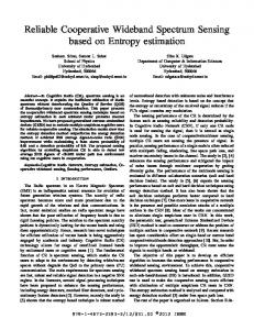
In this chapter, a novel technique is proposed for the problem of jointly estimating carrier frequency and single DoA of di↵erent PUs. The signals of PU sources are considered as uncorrelated band-limited signals.These sources are supposed to be spread over a wideband spectrum, and hence the proposal is applied on a wideband spectrum. The proposal is based on nonlinear KFs and an L-shaped uniform array, Two di↵erent algorithms are proposed using EKF and UKF. In section 4.1, the L-shaped array model are described. Section 4.2 presents the proposed state space model for this problem. The proposed algorithms are discussed in sections 4.3 and 4.3. Moreover, simulation results and a comparative study are delivered in section 4.5. Finally, conclusions are derived in section 4.6.

4.1

System Model

Since two di↵erent parameters should be estimated for each existing source signal, a 2D array should be used to accomplish this target. Thus, a traditional L-shaped uniform array, where two ULAs are connected together as shown in Figure 4.1, is considered to provide the 1

This chapter is a part of a published journal manuscript [92].

33

Chapter 4

Joint DoA & Carrier Freq. Estimation z

ml (t)

N . . . . . . 1 ✓l x 0

1

. . . . . .

N

Figure 4.1: L-shaped uniform array model proposed algorithm with the measurements. The first ULA is located on the x-axis and the other one is on the z-axis. Each array has N elements including the connecting one located on the corner of the L shape, i.e., the whole number of elements is 2N-1. The connecting element is considered as a reference point for both two arrays. Suppose L uncorrelated band-limited source signals are transmitted on separate carrier frequencies. The source signals are incident on the arrays with di↵erent DoAs. Thus, each element in both two arrays receives delayed versions of the source signals received by the reference point. Then, the output at nth element of the x-array and z-array respectively is defined by [93] rxn (t)

=

rzn (t) =

L X l=1 L X

ml (t)e

j2⇡(n 1)d

sin ✓l l

+ ⌘xn (t) (4.1)

ml (t)e

j2⇡(n 1)d

cos ✓l l

+ ⌘zn (t)

l=1

where ml (t), with l = 1, 2 . . . L, denotes the signal transmitted from the lth source and arrives the two arrays with a wavelength of l and a direction of arrival of ✓l . The element spacing in both two arrays is denoted as d. In addition, ⌘xn (t) and ⌘zn (t) denote noise signals in the nth element of the x-array and z-array respectively. Both ⌘xn (t) and ⌘zn (t) are assumed to be complex Gaussian white noise with zero mean and variance of n2 . In cognitive radio, SUs do not have any prior information about PUs being detected. The number of PUs is even unknown and then SUs have to blindly detect carrier frequencies and their corresponding DoAs. Thus, the problem being solved in this chapter is to find both carrier frequency and DoA for every source signal arrives the arrays 34

Joint DoA & Carrier Freq. Estimation

Chapter 4

while the measured outputs at both two arrays are the only known information. In the following section, a detailed description of how the proposed state space model is derived from Equation 4.1 is presented.

4.2

Proposed State Space Model

Each source signal is exposed to the same time delay between any two successive elements in the array. An lth source signal that reaches the nth element of both two arrays can be determined from its version that reaches the previous element respectively Xln = e

j2⇡d

Zln

j2⇡d

=e

sin ✓l l cos ✓l l

Xln

1

(4.2)

Zln 1

where Xln and Zln are the signals of the lth source received by the nth element of the x-array and z-array respectively. Equation 4.2 obviously represents a state space model in the spatial domain. Exploiting the spatial domain gives an advantage over the temporal state space, as there is no need to capture more than one time sample. Consequently, there is no need to use a high-speed ADC in capturing wideband spectrum. In other words, the proposed sensing technique can still successfully detect a wideband spectrum without requiring any additional hardware complexity. Both Xln and Zln , where l = 1, 2 . . . L, are complex signals, so each one can be decomposed into two real variables that represent real and imaginary values. Suppose Xln = xn2l 1 + jxn2l , then Equation 4.2 can be redefined as 2 3 ⇣ ⇣ sin ✓l ⌘ sin ✓l ⌘ 2 2 n 3 3 sin 2⇡d cos 2⇡d x2l 1 7 xn2l 11 6 l l 74 5 4 5=6 (4.3) 6 7 ⇣ ⌘ ⇣ ⌘ 4 5 n 1 n sin ✓l sin ✓l x2l x2l sin 2⇡d cos 2⇡d l

l

n n Similarly, suppose Zln = z2l 1 + jz2l , then 2 3 ⇣ ⇣ cos ✓l ⌘ cos ✓l ⌘ 2 2 n 3 3 cos 2⇡d sin 2⇡d n 1 z2l 1 z 6 7 l l 7 4 2l 1 5 4 5=6 6 7 ⇣ ⇣ 4 n 1 n cos ✓l ⌘ cos ✓l ⌘5 z2l z2l sin 2⇡d cos 2⇡d l

l

35

(4.4)

Chapter 4


Thus, the state variable xs 2 R4L⇥1 is formed at any element as a concatenation of real and imaginary values of the L source signals that arrive this element in the x-array followed by their versions arrive the corresponding z-array element, i.e., xs = [xr zr ]T where xr = [x1 x2 . . . x2L 1 x2L ]T and zr = [z1 z2 . . . z2L 1 z2L ]T . While KF is going to predict the posterior state variable in the spatial domain, it is assumed to predict the unknown DoAs and carrier frequencies as well. So, the state variable expands to contain these parameters. Thus, the state variable becomes xs = [xr zr A B]T where xs 2 R6L⇥1 and the column vectors A and B are described as A = [A1 . . . AL ]T =

h sin ✓

1

...

1

T

B = [B1 . . . BL ] =

h cos ✓ 1

sin ✓L iT L

1

...

cos ✓L iT

(4.5)

L

The parameters sinl✓l and cosl✓l are selected instead of directly selecting ✓l and l as state parameters. The reason is that these parameters share the same small range and can prevent sub-optimal filters from divergence. Moreover, the inter-element spacing d is set to a fraction of the minimum wavelength that can be estimated. Reducing d as possible can result in expanding the sinusoidal models in Equations 4.3 - 4.4 regarding to the unknown parameters. This, in turn, leads the filter to searching for the true values in a small region where the model is relatively linear. Under this scenario, both EKF and UKF can overcome their sub-optimal performance as discussed in section 3.2. Now, the process model of the spatial state space model can be formed 2 3 ↵x 0 0 0 6 0 ↵z 0 0 7 n 1 7x xns = 6 (4.6) 40 0 I 05 s 0 0 0 I where I 2 RL⇥L is the identity matrix. The matrices ↵x and ↵z 2 R2L⇥2L are defined as 2 3 2 3 ↵x1 0 0 ↵z1 0 0 6 7 6 7 ↵x = 4 0 . . . 0 5 , ↵z = 4 0 . . . 0 5 (4.7) 0 0 ↵xL 0 0 ↵zL 36

Joint DoA & Carrier Freq. Estimation where

2

6 6 ↵xl = 6 4

⇣

cos 2⇡d

sin ✓l ⌘

Chapter 4

⇣

sin 2⇡d

l

⇣

sin ✓l ⌘

⇣

sin ✓l ⌘

3

7 7 7 ⌘ sin ✓l 5 l

sin 2⇡d cos 2⇡d l l 2 3 ⇣ ⇣ cos ✓l ⌘ cos ✓l ⌘ cos 2⇡d sin 2⇡d 6 7 l l 6 7 ↵zl = 6 7 ⇣ ⌘ ⇣ ⌘ 4 cos ✓l cos ✓l 5 sin 2⇡d cos 2⇡d l

(4.8)

l

with l = 1, 2, . . . L. The second equation forming the state space model is the measurement model. Measurement model represents the output of the nth element in both two arrays. The real and imaginary values of the output of the nth element in the x-array can be deduced as n Yx,re

=

n Yx,im =

L X l=1 L X

xn2l

1

+ unx,re (4.9)

xn2l + unx,im

l=1

where unx,re and unx,im are the real and imaginary values of Gaussian white noise signal ⌘xn . The same is applied to z-array. Thus, measurement model in matrix notation becomes n n n n Yn = [Yx,re Yx,im Yz,re Yz,im ]T

2

1 60 =6 40 0

0 1 0 ... 0

1 0 0 0

0 1 0 0

0 0 1 0

0 0 0 ... 1

0 0 1 0

0 0 0 1

0 0 0 ... 0

3 0 (4.10) 07 n 7 x + un 05 s 0

The nonlinear process model and linear measurements model in Equation 4.6 and 4.10 respectively can be gathered in a state space model, where the process state model is similar to the one in Equation 3.1 and the measurements state model is similar to the one in Equation 3.2, as follows xns = f (xns 1 ) Yn = H xns + un 37

(4.11)

Chapter 4


where f (.) is the nonlinear function represents the system and un represents the measurements noise where un ⇠ N (0, R). The observation matrix H 2 R4⇥6L is constant over iteration in the proposed state space. The measurements noise covariance matrix R represents uncertainty in measurements due to noise signal. However, the process noise covariance matrix Q is assumed to be zero giving full trust in the proposed state space model. Since the state space model represents a nonlinear system, traditional linear KF would be inefficient at evaluating optimal estimate. Thus, sub-optimal EKF and UKF are recommended to deal with nonlinearity in this problem.

4.3

Proposed EKF-Based Approach

The main concept of EKF is that it linearizes the nonlinear system about the estimated trajectory. The linearization is performed using Taylor series and approximated to the first order partial derivatives along the trajectory. This, in turn, leads to degraded accuracy for strong nonlinear systems. Since the filter updates the estimated trajectory every iteration depending on measurements, partial derivatives, in turn, follow observed measurements. As a result, EKF is exposed to tremendous errors caused by linearization approximation and influence of noisy measurements on partial derivatives. The errors accumulate over iterations and eventually lead the filter to diverge. Since EKF is a sub-optimal filter and may fail to converge to true values, the filter can be encouraged to converge to the true carrier frequencies and DoAs if the criteria in section 3.2.3 is exploited. In other words, the parameters to be estimated are selected to have small variances relative to a region where the system is relatively linear. As a result, the linearized model approaches the original nonlinear model over a small operating range resulting in small linearization errors. In addition, initializing EKF with a value close to the mean value of the state parameters encourages the filter to operate in the target linear range. Besides, tuning the filter with selecting a suitable R leads to overcome the e↵ect of noisy measurements. As a result, EKF tends to approach the performance of traditional KF under these conditions. Consequently, the state parameters are supposed to relate to carrier frequencies and DoAs and have small variances as well. Thus, sinl✓l and cosl✓l are selected as mentioned in Equation 4.5. Now, EKF can be applied to the state space model described in 38


Chapter 4

Equations 4.6 and 4.10 to estimate the state variable xs . First, EKF ˆ 0 = E[xs ] and initial covariance is initialized with initial estimate x T ˆ 0 )(xs x ˆ 0 ) ]. Then, it predicts the posterior matrix P0 = E[(xs x ˆ n and posterior covariance matrix Pn from the previous estimates x state. The filter finally updates the estimates depending on observed measurements at the array elements. The filter goes through multiple iterations till the filter convergence. Every iteration consists of two steps as follows.

4.3.1

Prediction Step

ˆ n and covariance matrix Pn are predicted The posterior estimates x as described in [89] with ˆ n = f (ˆ x xn 1 )

(4.12)

Pn = Fn Pn 1 FTn

where Fn is Jacobian matrix of f (.) and contains the first order partial derivatives of f (xns ). 2 3 f1 0 f3 0 6 0 f2 0 f4 7 @f (xns 1 ) 6 7 Fn = = (4.13) @xns 1 xns 1 =ˆxn 1 4 0 0 I 0 5 0 0 0 I

where I 2 RL⇥L is the identity matrix. f1 , f2 , f3 and f4 are defined as follows 2 3 2 3 .. .. . 0 . 0 0 0 6 7 6 7 0 0 0 f1 = 4 0 , f = 5 4 5 2 1l 2l .. .. . . 0 0 0 0 2 3 2 3 ... ... 0 0 0 0 6 7 6 7 0 5, 0 5, f3 = 4 0 f4 = 4 0 l = 1, 2, . . . L 3l 4l .. .. . . 0 0 0 0 (4.14)

1l

2

@xn2l 1 6 @xn 1 6 2l 1 =6 6 4 @xn2l @xn2l 11

3 @xn2l 1 @xn2l 1 7 7 7 7 n 5 @x2l @xn2l 1 xns

2

1

=ˆ xn

1

6 =6 4 39

⇣

cos 2⇡dAˆnl ⇣

sin 2⇡dAˆnl

1

⌘

sin 2⇡dAˆnl

1

cos 2⇡dAˆnl

⌘

⇣

⇣

(4.15)

1

⌘3

1

7 7 ⌘5

Chapter 4

2l


2

n @z2l 1 6 @z n 1 6 2l 1 =6 6 n 4 @z2l n 1 @z2l 1

3l

@xn2l n 1 @z2l

3 @xn2l 1 6 @An 1 7 6 l 7 7 =6 6 7 n 4 @x2l 5 @Anl 1 xns 6 = 2⇡d 6 4 2

2

1 17

2

2

4l

3

n @z2l n @z2l

7 7 7 5

1

xn s

=ˆ xn

1

=ˆ xn

1

6 =6 4

⇣ ˆn sin 2⇡dB l

⇣ ⌘3 ˆn 1 sin 2⇡dB l 7 7 ⌘ ⇣ ⌘5 1 ˆn 1 cos 2⇡dB l

1

⇣

sin 2⇡dAˆnl ⇣

cos 2⇡dAˆnl 3

(4.16)

(4.17) 1

⌘

1

⇣

⌘

n @z2l 1 6 @B n 1 7 6 l 7 7 =6 6 7 n 4 @z2l 5 @Bln 1 xns 1 =ˆxn 1 ⇣ ⌘ 2 ˆn 1 sin 2⇡dB l 6 6 = 2⇡d 4 ⇣ ⌘ ˆn 1 cos 2⇡dB

⌘ 3

2 n 13 7 xˆ2l 1 74 5 ⇣ ⌘5 n 1 xˆ2l sin 2⇡dAˆnl 1

cos 2⇡dAˆnl

⇣

ˆn cos 2⇡dB l ⇣ ˆn sin 2⇡dB l

l

4.3.2

⇣ ⌘ ˆn 1 cos 2⇡dB l

1

1

⌘ 3

(4.18)

2 n 13 7 zˆ2l 1 74 5 ⌘5 n 1 1 zˆ2l

Updating Step

The posterior estimates are updated depending on the di↵erence beˆ n and the observed measuretween the estimated measurements H x th ments at the n elements Yn . The updating step follows the following equations as in [89] Kn = Pn HT (R + H Pn HT ) ˆn = x ˆ n + Kn (Yn H x ˆn ) x Pn = Pn K n H P n

1

(4.19)

where Kn is Kalman gain. The matrix H can be deduced by comparing both Equations 4.10 and 4.11. When the filter converges, the 40

Joint DoA & Carrier Freq. Estimation parameters ✓l and

l,

with l = 1, 2 . . . L, can be then evaluated as ✓l = tan l

4.4

Chapter 4

1

⇣A ⌘ l

Bl sin ✓l = or Al

l

cos ✓l = Bl

(4.20)

Proposed UKF-Based Approach

In UKF, Gaussian distributed state is represented by a minimal set of carefully chosen sigma points. Sigma points capture both the mean and covariance of the state variable. Then, sigma points are propagated through the nonlinear system. The systems outputs corresponding to sigma points are used to perfectly recover Gaussian state. The state variable xs can be estimated using UKF as well from the state space model in Equation 4.6. UKF algorithm is first introduced in [91], which gives clear derivation of the algorithm. First, UKF ˆ a0 , a concatenation of the initial estimate x ˆ 0 and is initialized with x initial estimates of measurements noise. The initial covariance matrix Pa0 is initialized as well. ˆ a0 = [ˆ x xT 0]T 0 P0 0 Pa0 = 0 P

(4.21)

ˆ 0 )(xs x ˆ 0 )T ] and P is measurements noise where P0 = E[(xs x covariance matrix (equivalent to R in EKF). Then, the filter repeats the following steps till it converges.

4.4.1

Selecting Sigma Points

For a state variable of dimension M, UKF selects 2M+1 sigma points. Therefore, for 6L⇥1 state variable xs , 12L+1 sigma points are evaluated as in [91]. a 0,n 1

a i,n 1

ˆ an 1 x

=

a i,n 1

ˆ an =x

1

+

⇣p ⇣p

ˆ an =x

1

(6L + ⇤)Pn

1

(6L + ⇤)Pn

1

41

⌘

⌘i i

, i = 1, 2 . . . 6L , i = 6L + 1, . . . 12L

(4.22)

Chapter 4


where ⇤ represents scaling parameter and ⇤ = ↵2 (6L + ) 6L. The ˆ n and  is ⌘a parameter ↵ denotes the spread of sigma points around ⇣p x secondary scaling parameter (usually 0). The term (6L + ⇤)Pn 1

i

represents the ith row of the matrix square root, evaluated by Cholesky decomposition [94].

4.4.2

Prediction Step

Sigma points corresponding to the state variable only xi,n 1 , with i = 0, 1, . . . 12L, are then propagated through the nonlinear process ˆn . model to predict the posterior estimates x x i,n|n 1

= f(

x i,n 1 )

(4.23)

where f (.) is the nonlinear function representing the process model, shown in Equation 4.6. The posterior estimate and covariance matrix are then evaluated as weighted mean and covariance matrix of new sigma points [91]. ˆn = x

12L X

(m)

x i,n|n 1

wi

i=0

Pn =

12L X

(c)

wi

i=0

⇣

x i,n|n 1

ˆn x

⌘⇣

x i,n|n 1

ˆn x

⌘T

(4.24)

where the weights are evaluated in UKF algorithm as (m)

w0

(c)

w0

(m)

wi

⇤ 6L + ⇤ ⇤ = + (1 ↵2 + ) 6L + ⇤ 1 (c) = wi = , i = 0, 1, . . . 12L 2(6L + ⇤) =

(4.25)

where represents prior knowledge of the state distribution ( = 2 for Gaussian distribution). On the other hand, sigma points are propagated through measurements model to predict the posterior predicted measurements as well. i,n|n 1

=H

ˆn = y

12L X

x i,n|n 1 (m)

wi

i=0

42

+

n i,n|n 1

(4.26) i,n|n 1


4.4.3

Chapter 4

Updating Step

Like EKF, the posterior estimate and covariance matrix are updated depending on the di↵erence between observed measurements Yn and ˆ n as follows [91] the predicted measurements y Kn = Pxñ yñ Pyñ1yñ

Pyñ yñ = Pxñ yñ =

12L X

ˆn ) y

Pn = Pn

KTn

(c)

wi

i=0 12L X i=0


(c)

wi

⇣

⇣

Kn Pyñ yñ ˆn y

i,n|n 1

x i,n|n 1

ˆn x

⌘⇣ ⌘⇣

i,n|n 1

i,n|n 1

(4.27)

ˆn y ˆn y

⌘T ⌘T

(4.28)

When the filter converges, ✓l and l can be estimated as in Equation 4.20. Although UKF generally has a better performance than EKF, it has to calculate a large number of sigma points in every iteration. As a result, UKF requires high time of processing.

4.5

Results and Discussions

In this section, a numerical study is presented. The experiment setup is first described, and then the results are discussed. Finally, a comparison among the proposed algorithm and proposals in [76] and [80] is presented.

4.5.1

Experiment Setup

For simulations, the number of elements in each array is set to 200 (N = 200) with inter-element spacing of one tenth of the minimum wavelength. Suppose that the two arrays receive signals from 6 different band-limited uncorrelated sources (L = 6). The normalized carrier frequencies of the received source signals are {0.878, 0.523, 0.643, 0.313, 0.135, 0.96} and their corresponding DoAs are {45.7, 33.8, 21.4, 78.3, -10.6, 4.9} respectively. In addition, the SNR at the array elements is assumed to be 10dB. EKF and UKF are properly initialized and tuned to avoid filters ˆ 0 is preferably set around the mean value divergence. In both filters, x 43

Chapter 4


of xs . However, it is set to di↵erent values during simulations to examine and compare the performance of both two filters. On the other hand, P0 should be carefully assumed, as a lower P0 than its true value leads the filter to trust inaccurate estimates and neglect observed measurements. Thus, P0 is set to its true value through simulations. The last parameters to be tuned are R and P in EKF and UKF respectively. Noise variance in the arrays can be an indication of the value of R and P , but they cannot be set to zero.

4.5.2

Simulation Results

Monte-Carlo simulations have been executed over 500 snapshots for both EKF and UKF algorithms. First, the initial estimates were set to value that is close to the mean of the state variable. So, all the elements of xˆ0 were set to 0.05. Both EKF and UKF were able to efficiently detect all carrier frequencies and the corresponding DoA of all the source signals. The estimated normalized frequencies fˆN and [ are gathered in Table 4.1. Figure 4.2 shows the speed of angles DoA convergence of both EKF and UKF. Both EKF and UKF need less than 10 iterations to converge to the true values of DoA as shown in Figure 4.2a. However, EKF was about 3 times faster than UKF in converging to the true values of carrier frequencies as shown in Figure 4.2b. Since each iteration represents exploiting another array element, UKF needs more array elements than EKF to perfectly converge. As shown in Figure 4.3, both EKF and UKF succeeded to pair both carrier frequencies and their corresponding DoAs. According to simulations, EKF algorithm is 10 times faster than UKF. Although UKF Table 4.1: Actual and estimated DoAs and normalized carrier frequencies of 6 di↵erent sources

Actual 45.7 33.8 21.4 78.3 10.6 4.9

DoA( ) EKF 45.6992 33.6861 21.4303 78.2553 10.5389 4.9475

UKF 45.7 33.8013 21.3996 78.3012 10.6041 4.8995 44

Normalized Frequency Actual EKF UKF 0.878 0.523 0.643 0.313 0.135 0.96

0.8781 0.5231 0.6431 0.313 0.1351 0.9601

0.8781 0.5231 0.6431 0.313 0.135 0.9602


Chapter 4

80 Source EKF UKF

60

! ◦) DoA(

40

20

0

-20

-40 0

10

20

30

40

50

# of Iterations

(a) Estimated DoA 1 0.9 Source EKF UKF

0.8 0.7

fˆN

0.6 0.5 0.4 0.3 0.2 0.1 0 0

10

20

30

40

50

No. of Iterations

(b) Estimated normalized frequency

Figure 4.2: Estimated parameters over iterations is a derivatives-free algorithm, it takes more time in evaluating the required sigma points in every iteration. Since the number of sigma points depends on the number of source signals, the processing time of UKF may increase exponentially with the increase in the number of source signals. Another experiment has been executed to examine the e↵ects of initial estimates. In this experiment, the initial estimates were set to 0.5 and 0.8. Then, the root mean square error (RMSE) in the estimated DoAs and normalized wavelengths ˆ N has been evaluated over 500 snapshots. The results of all these cases are gathered in Figure 4.4. When the initial estimate was set to 0.05 which is close to the mean value, both EKF and UKF gave the lowest RMSE in all cases. Then, RMSE tends to increase with the increase in the initial 45

Chapter 4

Joint DoA & Carrier Freq. Estimation 1 0.8 Actual EKF UKF

fˆN

0.6 0.4 0.2 0 -50

0

50

100

! DoA

Figure 4.3: Joint estimated carrier frequency and DoA using EKF and UKF estimates. The reason of this degradation is the sub-optimality of EKF and UKF, and hence they may converge to a sub-optimal solution if they are not properly initialized. To examine the e↵ects of the inter-element spacing on the performance of EKF and UKF, the simulation was repeated with an interelement spacing of min /4 and an initial estimate of 0.05. Figure 4.5 shows the di↵erence between the two cases where the inter-element spacing was min /4 and min /10. In Figure 4.5a where the interelement spacing was min /10, both EKF and UKF perfectly converged to the true values. When the inter-element spacing increased to one fourth of the minimum wavelength, the performance widely degraded as shown in Figure 4.5b. This proves the criteria discussed in section 3.2.3. When the inter-element spacing decreases the process state model expands to an extent in which it tends to be relatively linear regarding to the unknown state parameters. As a result, the linearization errors diminish and the performance of EKF almost approaches the performance of UKF. In contrast, the performance of EKF dramatically deteriorated compared to the performance of UKF when the inter-element spacing increases because of the linearization errors. The main drawback of the proposed algorithms in this chapter is their limited degrees of freedom. The proposed algorithms can detect a number of source signals up to the number of the elements in one ULA of the employed array. Thus, the structure used in these simulations was able to detect up to 199 sources. Since spectrum sensing techniques should be blind, the proposed algorithms should be set to detect the maximum possible number of sources (L = 199). When the 46


10 3

EKF,initial=0.05 EKF,initial=0.5 EKF,initial=0.8 UKF,initial=0.05 UKF,initial=0.5 UKF,initial=0.8

10 2

! ◦) RMSE in DoA(

10 1

10

Chapter 4

0

10 -1 10 -2

10

-3

10

-4

0

50

100

150

200

# of Iterations

(a) RMSE in estimated DoA 10 2 EKF,initial=0.05 EKF,initial=0.5 EKF,initial=0.8 UKF,initial=0.05 UKF,initial=0.5 UKF,initial=0.8

10 1

ˆN RMSE in λ

10 0 10 -1 10 -2

10 -3 10 -4 0

50

100

150

200

# of Iterations

(b) RMSE in estimated normalized wavelength

Figure 4.4: RMSE in estimated parameters at di↵erent initial estimates filter converges to the true values, the actual number of sources can be detected easily as the remaining signals would be converged to zero indicating their absence.

4.5.3

Comparative Study

For the sake of comparison, Kumar et al. [76] and Ariananda and Leus [80] are considered. These two algorithms depend on sub-Nyquist sam47

Chapter 4

Joint DoA & Carrier Freq. Estimation 1 0.8 Actual EKF UKF

fˆN

0.6 0.4 0.2 0 -50

0

50

100

! DoA

(a) d =

min /10

1.2 1

fˆN

0.8 0.6 0.4

Actual EKF UKF

0.2 0 -50

0

50

100

! DoA

(b) d =

min /4

Figure 4.5: Estimated DoA and carrier frequencies at di↵erent interelement spacing pling and have employed di↵erent array structures with a large number of ADCs to achieve sub-Nyquist rates. In [76], the authors have exploited a 2D nested array. The 2D nested array is a concatenation of two rectangular arrays, a dense rectangular array and a sparse one. Each element in the dense array is followed by a direct path with an ADC, while each element in the sparse array is followed by two paths and two ADCs. In [80], the employed array is a multi-coset array in which each element is followed by severe channels and each channel has a single ADC. The employed array can be considered as an Ns virtual ULA while N elements only are activated from the virtual array. Table 4.2 shows the di↵erences in degrees of freedom, sampling rate and the number of employed ADCs among them and the proposed 48

49 1

Ns M s

Ns M s B ⇤

for an N activated elements in an Ns virtual ULA

2Ns 1

(3N + 1) 2

(3N + 1)B 2

for a 2D nested array with N elements

4

l N m2

1

2N

1

No restrictions

for an (2N-1) L-shaped uniform array

N

Spectrum cannot be reconstructed since the system consider a single sample.

like [76], estimated parameters are evaluated numerically, leading to precise estimations.

KF-Based Proposed Approaches

* Ms denotes number of channels of multi-coset sampler and B denotes bandwidth of band-limited source signals.

# of ADCs employed

Minimum Sampling Rate

Degrees of Freedom

Discussion

Kumar et al. [76]

Reconstructed power spectrum is a It gives precise estimation since predefined grid where estimated estimated parameters are evaluated parameters are approximated to the numerically. nearest values. Wideband spectrum is compeletly reconstructed.

Ariananda and Leus [80]

Table 4.2: Comparison among the proposed algorithms and two other methods from the literature

Joint DoA & Carrier Freq. Estimation Chapter 4

Chapter 4


algorithm. Ariananda and Leus [80] has the highest degrees of freedom among the three algorithms. Since the increase in the number of the virtual elements Ns is faster than the increase in the number of the actual array elements N, Ariananda and Leus [80] can detect a large number of source signals with a few number of array elements [29]. For example, Ariananda and Leus [80] has degrees of freedom of more than 250 using 20 array elements only. However, Kumar et al. [76] and the proposed algorithm can result in degrees of freedom of 24 and 9 respectively using the same number of array elements. Kumar et al. [76] has the second highest degrees of freedom, which increase in a quadrature manner. As a result, when the number of array elements exceeds 13, the algorithm starts to detect a number of source signals higher than the employed array elements. However, the proposed algorithm has the lowest degrees of freedom, which increase linearly and cannot exceed the number of array elements as it depends on a dense array. On the other hand, the proposed algorithm has the simplest hardware requirement since a single time sample is required. Since the proposed algorithm exploits the spatial domain, there is no restrictions on the sampling rates. Then, a number of ADCs equal to the number of array elements are sufficient to capture one time sample. However, the other algorithms relying on sub-Nyquist rates require a large number of relaxed ADCs, which have restricted minimum sampling rates. Kumar et al. [76] requires a number of ADCs equal to 1.5 times the number of array elements. Thus, it has the second simplest hardware. However, Ariananda and Leus [80] requires a number of ADCs depending on Ns . Since the ratio N/Ns decreases with the increase in N, it results in an increasing number of ADCs and a more complex hardware architecture for larger problems.

4.5.4

Performance Evaluation

The performance of the proposed algorithms is compared to the performance of Kumar et al. [76] to evaluate their e↵ectiveness as a solution for the considered problem. The results are shown in Figure 4.6, with both EKF and UKF being executed with initial estimate of 0.05 and inter-element spacing of one-tenth of the minimum wavelength. Since the filters should be tuned at di↵erent SNRs by trial and error, the quality of tuning cannot be maintained fixed. Moreover, the shown results constitute the best performance that we were able to get by 50


Chapter 4

Figure 4.6: Overall RMSE of the proposed algorithms and Kumar et al. [76] manual tuning. However, there is no guarantee that lower RMSE cannot be accomplished. This raises the need to propose an optimization algorithm in the future for defining the point of the lowest RMSE. As a result, we avoid holding quantitative comparisons as long as possible. However, the proposals show a higher performance with lower RMSE than Kumar et al. [76] when simulations were executed at 5, 15 and 31dB as shown in Figure 4.6. The high performance at low SNRs is reasonable as KFs are designed to e↵ectively handle noisy measurements. Even though the performance of the proposed algorithms shows a competitive manner, it should be considered precisely and deliberately using an optimization algorithm in a future work.

4.6

Conclusions

In this chapter, two di↵erent approaches are proposed for the joint DoA and carrier frequency estimation problem using EKF and UKF. Both two filters were proven to be convenient for detecting the required parameters. Through simulations, UKF showed a lower RMSE than EKF, but higher processing time. Overall, the performance of both of them can be boosted using a number of factors. First of all, the filter initialization is a crucial factor that can enhance the performance. If the initial estimates are set close to the mean value of the parameters, the performance of EKF and UKF markedly improves. Second, the 51

Chapter 4


filter tuning is another factor that can help the filter to wisely follow the process and measurement models. That can be accomplished by setting the matrices R and P by trial and error till the filters converge with the lowest RMSE, while the matrix Q is assumed to be zero to reduce the complexity resulted from the trial-and-error process giving full trust to the process model. Third, choosing the estimated parameters to have the same range helps the filters to converge to the true values. Finally, the inter-element spacing plays a vital role in improving the performance of the proposals. Since reducing the inter-element spacing expands the process model and makes the filters operate on a region where the process model is piecewise linear. However, the main problem of the proposals is the limited degrees of freedom, as they are restricted to half of the whole number of the employed array elements.

52

Chapter 5 Joint 2D-DoA and Carrier Frequency Estimation Technique Using Nonlinear KFs 1

In this chapter, the proposal in chapter 4 is extended to detect a second angle along with DoA and carrier frequency. For this purpose, two Lshaped uniform arrays are employed, and nonlinear KFs are applied in the spatial domain. In section 5.1, the two L-shaped array model is described. Section 5.2 presents the proposed state space model for this problem. The proposed approaches are discussed in sections 5.3 and 5.4, while simulation results are delivered in section 5.5.

5.1

System Model

Since a 2D array was sufficient to detect two unknown parameters in the proposal of chapter 4, a 3D array would be e↵ective in detecting three di↵erent parameters of the source signals for the problem considered in this chapter. Therefore, two traditional L-shaped uniform arrays located in x-z plane and the y-z plane, as shown in Figure 5.1, are chosen to help formulate the proposed state space model. Each single ULA in this structure has N elements with an inter-element spacing of d. The element at the origin is considered as a reference point. Suppose that L di↵erent band-limited signals from L di↵erent 1

This chapter is a part of a published journal manuscript [95].

53

Chapter 5

Joint 2D-DoA & Carrier Freq. Estimation z

ml (t)

N . . . . . . 1 ✓l y 1

0

1

. . . . . .

N

. . .

l

. . .

N x

Figure 5.1: Two L-shaped uniform array model uncorrelated sources are impinging on the two L-shaped arrays. Each source signal is transmitted from a di↵erent direction on a di↵erent carrier frequency. Then, the output of each element can be evaluated as [93] rxn (t)

=

L X

ml (t)e

j2⇡(n 1)d

cos l sin ✓l l

ml (t)e

j2⇡(n 1)d

sin l sin ✓l l

ml (t)e

j2⇡(n 1)d

+ ⌘xn (t)

l=1

ryn (t) = rzn (t) =

L X l=1 L X

cos ✓l l

+ ⌘yn (t)

(5.1)

+ ⌘zn (t)

l=1

where rxn (t), ryn (t) and rzn (t) are the output of the nth element in the ULA located on x-axis, y-axis and z-axis respectively. The signal ml (t), with l = 1, 2 . . . L, denotes the received source signal at the reference point from the lth source. The signal ml (t) has a wavelength of l and arrives from a direction with an azimuth angle of l and an elevation angle of ✓l . Noise signals ⌘xn (t), ⌘yn (t) and ⌘zn (t) are assumed to be complex Gaussian white noise with zero mean and variance of 2 n. Since CRs are not allowed to have any prior information about licensed users being detected, the considered problem is a blind estimation problem. CR has to blindly estimate carrier frequency and the corresponding 2D-DoA of the surrounding PUs. For this problem, Kalman filter is proposed for estimating l , l and ✓l of each PU. 54

Joint 2D-DoA & Carrier Freq. Estimation

5.2

Chapter 5

Proposed Spatial State Space Model

The problem that confronts WBSS is the high hardware complexity required to perform sampling at Nyquist rates. Since the array geometry provides an opportunity to exploit the spatial domain, the proposed algorithms depends on a spatial state space instead of a temporal state space. The spatial state space is formed from the time delay that each source signal encounters between any two successive array elements. The time delay is expressed as a phase shift between the di↵erent versions of the source signals arrive the elements. Therefore, the lth source signal that reaches nth element in the three di↵erent ULAs Xln , Yln and Zln can be determined as Xln = e

j2⇡d

cos l sin ✓l l

Yl n = e

j2⇡d

sin l sin ✓l l

Zln = e

j2⇡d

cos ✓l l

Zln

Xln

1

Yl n

1

(5.2)

1

In matrix notation, Equation 5.2 can be reformulated as follows 2 4

xn2l

1

xn2l

2

3

6 5=6 6 4

where xn2l larly, 2 4

n y2l

1

n y2l

1

⇣

sin 2⇡d

l

⇣ cos sin 2⇡d

l

cos 2⇡d

l

cos

3 sin ✓l ⌘ 2 3 n 1 x 7 l 7 4 2l 1 5 7 cos l sin ✓l ⌘5 xn2l 1

sin ✓l ⌘

sin ✓l ⌘

l

⇣

l

l

(5.3) and xn2l represent real and imaginary parts of Xln . Simi-

2

3

⇣ cos cos 2⇡d

6 5=6 6 4

3 sin ✓l ⌘ 2 3 cos 2⇡d sin 2⇡d n 1 y 7 2l 1 l l 74 5 7 ⇣ ⌘ ⇣ ⌘ 5 n 1 sin l sin ✓l sin l sin ✓l y2l sin 2⇡d cos 2⇡d ⇣

sin

l

sin ✓l ⌘

⇣

sin

l

l

l

(5.4)

and 2 4

n z2l n z2l

1

3

2

6 5=6 6 4

3 ⇣ cos ✓l ⌘ 2 3 sin 2⇡d n 1 z 7 l l 7 4 2l 1 5 7 ⇣ ⇣ n 1 cos ✓l ⌘ cos ✓l ⌘5 z2l sin 2⇡d cos 2⇡d

⇣ cos ✓l ⌘ cos 2⇡d l

l

55

(5.5)

Chapter 5


The state variable xs 2 R6L⇥1 is then formed at any element as a concatenation of the real and imaginary values in the three ULAs as follows xs = [x1 , x2 . . . x2L 1 , x2L , y1 , y2 . . . y2L 1 , y2L , z1 , z2 , . . . z2L 1 , z2L ]T (5.6) Since KFs are considered to predict unknown parameters, these parameters should be concatenated to the state variable. Then, in each iteration of the kalman filtering, the parameters are estimated as well as the posterior estimate of the state variable. The parameters to be estimated in the considered problem are carrier frequency, azimuth and elevation angles of the L sources. These parameters are not going to be concatenated to the state variable directly as they vary over di↵erent wide ranges and may force EKF to diverge. So, related parameters that share the same range are selected instead to speed up the filter convergence and boost the filter performance. The parameters are selected to be al =

cos

l

sin ✓l

, bl =

l

sin

l

sin ✓l l

cl =

cos ✓l

(5.7)

l

where l = 1, 2 . . . L. By estimating these parameters using KF, l , ✓l and l can be evaluated for each source. Moreover, the inter-element spacing d is set to a fraction of the minimum wavelength that can be estimated. Reducing d as possible can result in expanding the sinusoidal model in Equations 5.3 - 5.5 regarding to the unknown parameters. This, in turn, leads the filter to searching through a region where the model is relatively linear. Under this scenario, both EKF and UKF can overcome their sub-optimal performance and converge to more precise values as discussed in section 3.2.3. Using simulation in section 5.5, an enhanced performance is proven while decreasing d. Now, the state variable becomes xs 2 R9L⇥1 and the process model of the spatial state space model can be defined 2 3 ↵x 0 0 0 0 0 6 0 ↵y 0 0 0 07 6 7 60 0 ↵ z 0 0 07 n 6 7 xns 1 xs = 6 (5.8) 7 0 0 0 I 0 0 6 7 40 0 0 0 I 05 0 0 0 0 0 I 56


Chapter 5

where I 2 RL⇥L is the identity matrix. The submatrices ↵x , ↵y and ↵z 2 R2L⇥2L are defined as 2

↵x1

6 ↵x = 4 0 0

0 .. . 0

0

3

2

↵y1

7 6 0 5 , ↵y = 4 0 ↵xL 0

0 .. .

3

0

2

↵z1

7 6 0 5 , ↵z = 4 0 ↵yL 0

0

0 .. .

0

7 0 5 0 ↵zL (5.9)

where 2

6 6 ↵xl = 6 4 2

6 6 ↵yl = 6 4 2

6 6 ↵zl = 6 4

⇣ cos cos 2⇡d ⇣

sin 2⇡d ⇣

cos 2⇡d ⇣

cos 2⇡d

sin ✓l ⌘

⇣ cos sin 2⇡d

l

cos 2⇡d

l

cos

sin ✓l ⌘

⇣

l

sin

l

sin ✓l ⌘

sin

l

sin 2⇡d

sin ✓l ⌘

cos ✓l ⌘ l

⇣

sin 2⇡d

⇣ ⇣ cos ✓l ⌘ sin 2⇡d cos 2⇡d l

sin ✓l ⌘

3

7 7 7 ⌘ cos l sin ✓l 5 l

sin

l

sin ✓l ⌘

⇣

3

7 7 7 sin l sin ✓l ⌘5 l

cos 2⇡d

l

l

l

⇣

l

sin 2⇡d ⇣

l

(5.10)

l

cos ✓l ⌘

3

7 7 7 ⌘ cos ✓l 5 l

l

with l = 1, 2, . . . L. However, the measurement model of the spatial state space represents the measured output at the nth element in all arrays. The measured output at the nth element is expected to be the sum of all incident source signals on this element. It, however, is exposed to measurement errors and hence the measurement model can be declared in 57

3

Chapter 5


matrix notation as n n n n n n Yn = [Yx,re Yx,im Yy,re Yy,im Yz,re Yz,im ]T

2

1 60 6 60 =6 60 6 40 0

0 1 0 ... 0 0 0

0 0 1 0 0 0

0 0 0 ... 1 0 0

0 0 0 0 1 0

0 0 0 0 0 1

0 0 0 ... 0 0 0

3 0 07 7 07 7 xns + un 07 7 05 0

(5.11)

n n n where Yx,re , Yy,re and Yz,re are the real parts of the nth element output in the x-array, y-array and z-array respectively. The remaining terms n n n , Yy,im and Yz,im are the imaginary parts of these outputs respecYx,im tively. The vector un represents the measurement noise signals which has zero-mean and covariance matrix R. The spatial state model is now formulated and it obviously contains a nonlinear process model as in Equation 3.2 and a linear measurement model as in Equation 3.1. Thus, sub-optimal EKF and UKF are proposed for the nonlinearity of this problem. While applying these filters to the proposed state model, the process noise covariance matrix Q is assumed to be zero giving full trust in the proposed process model.

5.3

Proposed EKF-Based Approach

The first approach proposes EKF algorithm in [89] for estimating the state variable xs from the state space model that has been already ˆ 0 and formulated. First, EKF is initialized with an initial estimate x ˆ 0 is preferable to be initial covariance matrix P0 . The initial estimate x selected close to the mean value of the state variable to speed up the convergence. Moreover, The matrix P0 should be carefully selected as it may be set to a low value that is enough to force the filter to fully trust the posterior estimates and neglect the e↵ect of measurements. Then, EKF goes through several iterations and each iteration consists of two steps: prediction step that follows the process model and updating step that follows the measurement model as shown in Algorithm 5.1. In each prediction step, the nonlinear process model must be linearized around the prior estimates. Then, the approximated resultant to the first order derivatives is calculated as a Jacobian matrix 58


Chapter 5

Fn

@f (xns 1 ) Fn = @xns 1

2

xn s

1

=ˆ xn

1

3 0 0 f4 0 0 f2 0 0 f5 0 7 7 0 f3 0 0 f6 7 7 0 0 I 0 07 7 0 0 0 I 05 0 0 0 0 I

f1 60 6 60 =6 60 6 40 0

Algorithm 5.1 EKF-based proposed algorithm 0: Intialization: ˆ 0 = E[xs ] x

0:

ˆ 0 )T ] x

ˆ 0 )(xs x

P0 = E[(xs loop: Prediction Step:

@f (xns 1 ) @xns 1 ˆ n = f (ˆ x xn 1 ) Fn =

xn s

1

=ˆ xn

1

Pn = Fn Pn 1 FTn Updating Step: Kn = Pn HT (R + H Pn HT ) ˆn = x ˆ n + Kn (Yn H x ˆn ) x Pn = Pn K n H P n if convergence: for each source: l

= tan

✓l = sin l

1

1

cos ✓l = cl

break loop 59

⇣b ⌘ l

al ⇣b ⌘ l

cl

1

(5.12)

Chapter 5


where I 2 RL⇥L is the identity matrix. The matrices f1 , f2 , f3 , f4 , f5 and f6 are defined as follows 2

..

6 f1 = 4 0

.

0

3 0 7 0 5, ...

0 1l

0

l = 1, 2, . . . L

(5.13)

where

1l

2

@xn2l 1 6 @xn 1 6 2l 1 =6 6 4 @xn2l @xn2l 11

3 @xn2l 1 @xn2l 1 7 7 7 7 n 5 @x2l @xn2l 1 xns

⇣ ⌘3 sin 2⇡dˆ anl 1 6 7 7 =6 4 ⇣ ⌘ ⇣ ⌘5 sin 2⇡dˆ anl 1 cos 2⇡dˆ anl 1 2

1

=ˆ xn

1

⇣ ⌘ cos 2⇡dˆ anl 1

(5.14) Similarly, the remaining matrices f2 , f3 , f4 , f5 and f6 are diagonal and their diagonals have the elements 2l , 3l , 4l , 5l and 6l respectively. In the same manner, they are evaluated as

2l

4l

5l

6l

2

6 =6 4

⇣

cos 2⇡dˆbnl ⇣

1

⌘

⇣

sin 2⇡dˆbnl

⌘

⇣

1

⌘3 7 7 ⌘5

sin 2⇡dˆbnl 1 cos 2⇡dˆbnl 1 ⇣ ⌘ ⇣ ⌘3 2 cos 2⇡dˆ cnl 1 sin 2⇡dˆ cnl 1 6 7 6 7 3l = 4 ⇣ ⌘ ⇣ ⌘5 sin 2⇡dˆ cnl 1 cos 2⇡dˆ cnl 1 ⇣ ⌘ ⇣ ⌘ 3 2 2 n 13 sin 2⇡dˆ anl 1 cos 2⇡dˆ anl 1 6 7 xˆ2l 1 74 5 = 2⇡d 6 4 ⇣ ⌘ ⇣ ⌘5 n 1 xˆ2l cos 2⇡dˆ anl 1 sin 2⇡dˆ anl 1 ⇣ ⌘ ⇣ ⌘ 3 2 2 n 13 sin 2⇡dˆbnl 1 cos 2⇡dˆbnl 1 6 7 yˆ2l 1 74 5 = 2⇡d 6 4 ⇣ ⌘ ⇣ ⌘5 n 1 yˆ2l cos 2⇡dˆbnl 1 sin 2⇡dˆbnl 1 ⇣ ⌘ ⇣ ⌘ 3 2 2 n 13 sin 2⇡dˆ cnl 1 cos 2⇡dˆ cnl 1 6 7 zˆ2l 1 74 5 = 2⇡d 6 4 ⇣ ⌘ ⇣ ⌘5 n 1 zˆ2l cos 2⇡dˆ cnl 1 sin 2⇡dˆ cnl 1 60

(5.15)


Chapter 5

After performing linearization by evaluating Jacobian matrix Fn , the ˆ n and covariance matrix Pn are predicted from posterior estimate x ˆ n 1 and Pn 1 respectively. The predicted estimates their prior values x are then updated depending on the filter gain Kn and observation matrix H as shown in Algorithm 5.1. The filter then goes through several iterations of prediction and updating, till it finally tends to converge. The filter converges to the true values of al , bl and cl since the estimated parameters have a small variance compared to a region where the model is relatively linear. This, in turn, forces EKF to approach the performance of traditional linear KF. The unknown carrier frequencies and 2D angles are finally calculated from the estimated al , bl and cl .

5.4

Proposed UKF-Based Approach

The second approach proposes UKF algorithm, described in [91], for the considered estimation problem. The complete algorithm is deˆ a0 and covariance scribed in Algorithm 5.2. First, the initial estimate x a ˆ a0 is a conmatrix P0 are initialized properly. The initial estimate x ˆ 0 and the initial catenation of the initial estimate of state variable x estimate of measurements noise. This, in turn, leads the initial covariance matrix Pa0 to gather both the covariance matrix of state variable ˆ 0 )(xs x ˆ 0 )T ] and the measurements noise covariance P0 = E[(xs x matrix P (equivalent to R in EKF). Then, the filter rotates in several iterations till the filter converges to the true values. In each iteration, sigma points ai,n 1 , with i = 0, 1 . . . 18L, are selected to perfectly capture the mean and variance of the state variable. Since a state variable of dimension M needs 2M+1 sigma points, the state variable xs needs 18L+1 sigma points. These sigma points are in Algorithm 5.2 by determining ⇣pevaluated as shown ⌘ th the i row of (6L + ⇤)Pn 1 using Cholesky decomposition. The i

parameter ⇤ is a scaling parameter which equals to ↵2 (6L + ) 6L ˆ n and  is a where ↵ denotes the spread of sigma points around x secondary scaling parameter (usually equals to 0). After selecting the sigma points, the filter executes prediction step in which the sigma points are propagated through the nonlinear process model, and the resultant is used to predict the posterior estimate ˆ n . The posterior estimate x ˆ n and covariance matrix Pn are evalux ated as weighted mean and covariance matrix of the resultant. The 61

Chapter 5


Algorithm 5.2 UKF-based proposed algorithm 0: Intialization: ˆ a0 x

=

[ˆ xT0

T

Pa0

0] ,



=

P0 0

0 P

0: loop: Selecting Sigma Points: a 0,n 1

a i,n 1

ˆ an 1 x

=

a i,n 1

ˆ an =x

+

⇣p ⇣p

1

Prediction Step:

ˆ an =x

1

⌘

(6L + ⇤)Pn

1

(6L + ⇤)Pn

1

x i,n|n 1

x i,n 1 )

12L X

ˆn = x

= f( (m)

⌘i i

, i = 1, 2 . . . 6L , i = 6L + 1, . . . 12L

x i,n|n 1

wi

i=0

Pn =

12L X

(c)

wi

i=0

⇣

x i,n|n 1

ˆn x

⌘⇣

x i,n|n 1

ˆn x

⌘T

Updating Step: i,n|n 1

x i,n|n 1

= Hn

ˆn = y

12L X

+

n i,n|n 1

(m)

wi

i,n|n 1

i=0

Pyñ yñ =

12L X

(c)

wi

i=0

Pxñ yñ =

12L X

(c)

wi

i=0

⇣ ⇣

i,n|n 1

ˆn y

x i,n|n 1

ˆn x

Kn = Pxñ yñ Pyñ1yñ

⌘⇣

⌘⇣


i,n|n 1

ˆn y

i,n|n 1

ˆn y

ˆn ) y

Kn Pyñ yñ KTn

Pn = Pn if convergence: for each source: l

= tan

1

⇣b ⌘ l

al l

,

=

✓l = sin cos ✓l cl

break loop

62

1

⇣b ⌘ l

cl

⌘T

⌘T


Chapter 5

employed weights is defines as in [89] (m)

w0

(c)

=

w0 =

(m)

wi

⇤ 6L + ⇤ ⇤ + (1 6L + ⇤ (c)

= wi =

↵2 + )

1 2(6L + ⇤)

(5.16)

i = 0, 1 . . . 18L

where represents the state variable distribution ( = 2 for Gaussian distribution). Then, the filter executes updating step where the posterior estimate and covariance matrix are corrected by the measurements. They are updated based on the di↵erence between the estimated observations yn and the actual measurements Yn . The estimated observations are evaluated as a weighted mean of the resultant of measurement model after the sigma points are propagated through it. The complete algorithm used in prediction and updating steps are shown in Algorithm 5.2. The filter keeps going in iterations of selecting the sigma points, prediction and updating, till it converges to the true values. Finally, The carrier frequencies, azimuth angles and elevation angles are evaluated. In fact, UKF tends to have a better performance than EKF, as UKF is accurate to the third order derivatives. Furthermore, UKF, unlike EKF, is a derivative-free filter. However, it requires calculating sigma points using Cholesky decomposition in every iteration. This leads UKF to have higher processing time.

5.5

Results and Discussions

Numerical simulations of the proposed approaches are presented in this section. First, the simulation model is presented, and then the simulation results and discussions are held. Finally, a comparison among the proposal in [76], [85] and the proposed algorithm is presented. 63

Chapter 5

5.5.1


Experiment Setup

For simulations, each ULA on each axis has 150 elements (N = 150) with an inter-element spacing of one-fourth of the minimum wavelength. Twelve di↵erent source signals are impinging on the arrays. The source signals are traveling from di↵erent angles and are carried on di↵erent carrier frequencies. Table 5.1 shows the carrier frequencies and their corresponding 2D-DoAs for the di↵erent sources. The SNR is selected to be 5dB. The initial estimates in both EKF and UKF are set to values that are close to the mean value of the state variable. Thus, all elements ˆ o are set to 0.03. The initial covariance in the initial estimate vector x matrix P0 is also set to a proper value which prevents the filter from fully trust the estimates and ignoring the observations. Thus, it is initialized with its true value. Then, the filters are tuned carefully to guarantee the filter convergence by trial and error.

5.5.2

Simulation Results

estimates. Under this scenario, Monte-Carlo simulations have been executed with both EKF and UKF for 500 snapshots. Both filters succeeded in detecting the carrier frequency and 2D-DoA of all source ˆ and norsignals. The RMSE in the estimated azimuth ˆ, elevation ✓, ˆ malized wavelength N is shown in Figure 5.2a, and the estimated parameters are gathered in Table 5.2. Although EKF and UKF are sub-optimal estimators, they successfully detect the di↵erent sources with RMSE in all the estimated parameters close to 10 1 . The reason is that the estimated values are located on the same range and the initial estimates are set to the center of that range. These factors helped the filters to converge to the true values. However, both Table 5.1: DoAs and normalized carrier frequencies of 12 di↵erent sources # of source

Azimuth ( )

Elevation ( )

Normalized Frequency

# of source

Azimuth ( )

Elevation ( )

Normalized Frequency

1 2 3 4 5 6

30 47 93 52 127 173

5 84 23 37 53 127

0.463 0.217 0.294 0.716 0.607 0.861

7 8 9 10 11 12

60 205 146 26 237 100

94 151 89 163 77 41

0.354 0.119 0.67 0.294 0.52 0.4

64


Chapter 5

EKF and UKF have showed a degraded performance when the initial estimates were set to 0.7. The RMSE in this case has deteriorated markedly as shown in Figure 5.2b. To explicitly declare those find-

EKF Azimuth UKF Azimuth EKF Elevation UKF Elevation

10 0

ˆ ◦) RMSE in φˆ and θ(


10 1

10 -1

10 -2

10

EKF Azimuth UKF Azimuth EKF Elevation UKF Elevation

2

10 1 10 -3 0

50

100

150

0

50

# of Iterations

100

10 0

10 1 EKF UKF

EKF UKF

10 -1

RMSE in λˆN

RMSE in λˆN

150

# of Iterations

10 -2

10 -3

10 0

10 -1 0

50

100

150

0

50

# of Iterations

100

150

# of Iterations

(a) Initial estimate = 0.03

(b) Initial estimate = 0.7

Figure 5.2: RMSE in the estimated azimuth, elevation and normalized wavelength Table 5.2: Actual and estimated 2D-DoAs and normalized carrier frequencies of 12 di↵erent sources Actual 30 47 93 52 127 173 60 205 146 26 237 100

Azimuth EKF 30.012 46.999 92.956 51.997 126.970 172.979 59.992 204.712 145.976 26.018 237.010 99.966

UKF

Actual

Elevation EKF

UKF

29.615 47.009 93.356 52.015 127.110 173.061 60.040 205.294 146.078 25.786 236.978 100.169

5 84 23 37 53 127 94 151 89 163 77 41

5.024 83.978 23.018 37.006 52.992 126.994 93.977 150.864 88.983 162.932 76.964 41.003

4.895 84.151 22.939 36.972 53.043 127.012 94.118 150.791 89.057 163.201 77.093 41.005

65

Normalized Frequency Actual EKF UKF 0.463 0.217 0.294 0.716 0.607 0.861 0.354 0.119 0.67 0.294 0.52 0.4

0.461 0.216 0.293 0.713 0.604 0.854 0.356 0.118 0.666 0.292 0.516 0.398

0.473 0.221 0.299 0.731 0.620 0.881 0.361 0.123 0.685 0.301 0.532 0.408

Chapter 5


200

200

150

150

100

100

θˆ

θˆ

ings, the estimated carrier frequency and 2D-DoA in the two cases are shown in Figure 5.3. In Figure 5.3a, the estimated parameters are obviously close to the actual values when the initial estimate is 0.03. However, when the initial estimate was set to 0.7, EKF converged to erroneous values which are far apart from the true values and UKF converged to the true values with massive errors as shown in Figure 5.3b. This proves that initial estimates play a crucial role in the filter convergence and may lead the filter to completely diverge if they are not set properly. Another thing can be found in Figure 5.2. When the initial estimate is 0.7, UKF outperforms EKF. That is expected, as UKF is accurate to the third order derivative while EKF is accurate to the first order derivative. However, EKF outperforms UKF when the initial estimate is 0.03. This indicates that the filter operates over a relatively linear model where the linearization error is massively reduced. This also reflects the vital role of initial The inter-element spacing of the array can enhance the performance of EKF and UKF. As reducing the inter-element spacing ex-

50

50

Actual EKF UKF

0

Actual EKF UKF

0 0

50

100

150

200

250

0

50

100

φˆ

150

200

250

φˆ

0.8

0.8

0.6

0.6

fˆN

1

fˆN

1

0.4

0.4

Actual EKF UKF

0.2

Actual EKF UKF

0.2

0

0 0

50

100

150

200

250

0

φˆ

50

100

150

200

250

φˆ

(a) Initial estimate = 0.03

(b) Initial estimate = 0.7

Figure 5.3: Estimated carrier frequencies and their corresponding 2DDoA 66


Chapter 5

pands the process model relating to the estimated parameters al , bl and cl . Expanding a nonlinear model can produce relatively linear characteristics over the region where those parameters are defined. This is proven by the improved performance accomplished by reducing the inter-element spacing. New experiment has been executed with an initial estimate of 0.7 to show the e↵ect of the inter-element spacing in a worse case. For di↵erent inter-element spacing values, simulations have been carried out and the results are shown in Figure 5.4. When the inter-element spacing is reduced to one-tenth of the minimum wavelength, the performance of both EKF and UKF is enhanced and the RMSE is reduced. Moreover, EKF performance starts to approach UKF performance and the gab between their performances is tremendously diminished. This indicates that linearization error has

10 3 EKF, d = λmin /4

EKF, d = λmin /4

UKF, d = λmin /4

UKF, d = λmin /4

UKF, d = λmin /10

10 2

10 1

10 0

0

50

100

EKF, d = λmin /10

10 2

ˆ ◦) RMSE in θ(

ˆ ◦) RMSE in φ(

EKF, d = λmin /10

150

UKF, d = λmin /10

10 1

10 0

0

50

# of Iterations

100

150

# of Iterations

(a) RMSE in azimuth

(b) RMSE in elevation EKF, d = λmin /4

10 1

UKF, d = λmin /4

RMSE in λˆN

EKF, d = λmin /10 UKF, d = λmin /10

10 0

10 -1

0

50

100

150

# of Iterations

(c) RMSE in normalized wavelength

Figure 5.4: RMSE in the estimated azimuth, elevation and normalized wavelength with initial estimates of 0.7 and di↵erent inter-element spacing 67

Chapter 5


been reduced and the process model tends to be relatively linear. Reducing the inter-element spacing, however, produces mutual coupling in the array elements. Another experiment has been carried out to find out the e↵ect of the number of source signals. The simulations have been repeated for 5, 12 and 24 source signals with inter-element spacing of min /10 and initial estimate of 0.03. The filters were still able to detect all the carrier frequencies with their corresponding elevation and azimuth angles as shown in Figure 5.5. The filters can continue to detect a larger number of sources up to the degrees of freedom of two L-shaped uniform arrays. The degrees of freedom are limited to the number of array elements in one axis. Thus, the maximum number of source signals that can be detected with this system is 149. Since the detection of PUs is a blind estimation problem in CR, the CRs have no prior information about the number of existing sources. In this case, the filters are set to detect 149 di↵erent source signals and finally detect the actual number of the sources, as the remaining signals would be zero. As depicted in Figure 5.5, the proposed approaches can detect azimuth angles up to 300 . As two L-shaped uniform arrays provide the ability to detect an azimuth angle of 360 and an elevation angle of 180 . In Figure 5.5c, There are many pairs that share the same frequency or the same elevation, but the two filters were able to distinguish between them since they di↵er in the other parameters. From simulations, it is found that EKF consumes time 20 times lower than the time consumed by UKF to detect 5 di↵erent sources. When the number of source signals is raised to 12, the ratio between the time consumed by UKF and EKF roughly becomes 40. Again, this ratio becomes around 70, when the number of sources becomes 24. Although UKF is a derivative-free filter, it consumes much time in selecting sigma points. Since the number of sigma points depends on the number of source signals, the time consumed by UKF to calculate and process these sigma points increases rapidly with the increase in the number of sources. A further experiment has been carried out to examine the proposals at di↵erent levels of SNRs. Thus, the simulations have been repeated with an initial estimate of 0.03 and inter-element spacing of one-tenth of the minimum wavelength. The SNR level was set to 1dB and 13dB respectively, and the RMSE in the estimated parameters was evaluated at each level. The results are gathered in Figure 5.6. At each SNR level, the filters should be tuned again to handle the new level of 68

Joint 2D-DoA & Carrier Freq. Estimation 90

80 Actual EKF UKF

80

Actual EKF UKF

70

70

60

60

50

Est. Elevation

Est. Elevation

Chapter 5

50 40

40 30

30

20

20

10

10

0 0

10

20

30

40

50

60

70

80

90

0

20

40

60

80

Est. Azimuth

1

140

160

180

200

Actual EKF UKF

0.9 0.8

Est. Normalized Frquency

0.8


120

1

Actual EKF UKF

0.9

0.7 0.6 0.5 0.4 0.3 0.2

0.7 0.6 0.5 0.4 0.3 0.2

0.1 0

100

Est. Azimuth

0.1 0

10

20

30

40

50

60

70

80

0

90

0

20

40

60

80

Est. Azimuth

100

120

140

160

180

200

Est. Azimuth

(a) L = 5

(b) L = 12

90

Actual EKF UKF

80 70

Est. Elevation

60 50 40 30 20 10 0 -50

0

50

100

150

200

250

300

Est. Azimuth

1

Actual EKF UKF

0.9


0.8 0.7 0.6 0.5 0.4 0.3 0.2 0.1 0 -50

0

50

100

150

200

250

300

Est. Azimuth

(c) L = 24

Figure 5.5: Estimated carrier frequencies and their corresponding 2DDoA for di↵erent number of sources

uncertainty in the measurements. The filter tuning is a trial-and-error process, where the matrix R is changed several times till the filter tends to converge. Therefore, the resultant RMSE follows both the SNR level and the quality of tuning as well. Overall, Figure 5.6 shows an improvement in the filter performance with the increase in SNR. 69

Chapter 5




10 1 EKF, Azimuth UKF, Azimuth EKF, Elevation UKF, Elevation

10 0

10 -1

0

50

100

10

10 -1

10 -2

10 -3

150

EKF, Azimuth UKF, Azimuth EKF, Elevation UKF, Elevation

0

0

# of Iterations

50

100

150

# of Iterations

10 0 EKF UKF

10 0

10 -1

RMSE in λˆN

RMSE in λˆN

EKF UKF

10 -2

10 -1

10 -2

10 -3

10 -3 0

50

100

150

0

# of Iterations

50

100

150

# of Iterations

(a) SNR = 1dB

(b) SNR = 13dB

Figure 5.6: RMSE in the estimated carrier frequencies and their corresponding 2D-DoA at di↵erent SNRs EKF still follows the same behavior as in Figure 5.3a and outperforms UKF because of selecting the initial estimate around zero and the small inter-element spacing.

5.5.3

Comparative Study

References [76] and [85] are considered for the sake of comparison. In [76], the authors have proposed a new architecture with a 2D nested array to implement sub-Nyquist sampling. The 2D nested array consists of two rectangular arrays: a sparse rectangular array and a dense one. To achieve sub-Nyquist rate, each element in the dense array is followed by a single ADC that samples the signals at sub-Nyquist rate. However, each element in the sparse array is followed by two paths: a direct path with an ADC and a delayed path with another ADC. Then, a proposed algorithm is executed to obtain the carrier frequency and a single DoA for each source. In [85], the authors have exploited a standard URA for detecting both the carrier frequency and the cor70


Chapter 5

responding 2D-DoA of each source. Then, the authors have proposed adding a number of delay channels after a single array element of the employed URA. Each delay channel has been provided with an ADC. Then, the authors have exploited the spatial and time delays to detect the unknown parameters using ESPRIT algorithm. In contrast, the proposal in this chapter does not rely on this large number of ADCs as the processing is executed spatially. Table 5.3 shows the di↵erences among the proposed algorithm, Kumar et al. [85] and Kumar et al. [76]. Kumar et al. [85] can detect a number of source signals higher than the number of array elements if the number of the employed delay channels exceeds 4. However, the simulations in [85] have proven that the higher the number of delay channels, the higher the performance would be accomplished. Thus, the number of delay channels would be twice or triple the number of array elements. In this context, the degrees of freedom of Kumar et al. [85] increase exponentially with the increase in the number of the employed array elements. Under these circumstances, it outperforms the proposed algorithm and Kumar et al. [76]. Although the latter has degrees of freedom that also increase exponentially, they rise at a slower rate than the degrees of freedom of Kumar et al. [85]. That is predictable since Kumar et al. [85], unlike the others, has no constraints on detecting a number of source signals higher than the number of the employed array elements. However, Kumar et al. [76] needed at least 5 array elements to start detecting source signals. Besides, it started to detect a number of source signals higher than the number of the employed array elements when the number of array elements exceeded 13. The proposed algorithm, however, started to detect signals with at least 4 array elements, and its degrees of freedom increase linearly with the increase of the array elements. Besides, its degrees of freedom are restricted to one-third of the total number of the employed array elements. Overall, the proposed algorithm has the lowest degrees of freedom among the three methods as it does not rely on sparsity on any domain. On the other hand, the proposed algorithm has employed a lower number of ADCs as there are no restrictions on the sampling rate. Since both Kumar et al. [76] and Kumar et al. [85] operate at subNyquist rates to sample a wideband spectrum, their implementations require a large number of relaxed ADCs. The number of ADCs required for Kumar et al. [76] is around 1.5 times the number of array elements. Kumar et al. [85] required a number of ADCs equal to 71

72

2D-DoA Carrier Frequency

Estimated Parameters

(3N + 1) 2 DoA Carrier Frequency

* B denotes the bandwidth of band-limited source signals.

N+M

# of ADCs employed

(3N + 1)B⇤ 2

NM 4

Degrees of Freedom (N + M)B⇤

A 2D nested array with N elements l N m2 1 4

A URA with N elements and M delay channels

Architecture

Minimum Sampling Rate

Kumar et al. [76]

Kumar et al. [85]

1

2 2D-DoA Carrier Frequency

3N

No restrictions

N

Two L-shaped uniform arrays with 3N 2 elements

KF-Based Proposed Approaches

Table 5.3: Comparison among the proposed approaches, Kumar et al. [85] and Kumar et al. [76]

Chapter 5 Joint 2D-DoA & Carrier Freq. Estimation


Chapter 5

the total number of the employed array elements and delay channels together. As a result, the number of ADCs may be 3 or 4 times the number of array elements, which can be considered as the price that has been paid for the high degrees of freedoms. However, the proposed algorithm exploits the spatial domain instead of the temporal domain to get rid of the need to sample the signals at Nyquist rates, and hence it only requires a number of ADCs equal to the number of the employed array elements without any restrictions on the speed of the ADCs. So, the number of ADCs required for the proposed algorithm is always lower than the number required by Kumar et al. [76] and Kumar et al. [85] for the same number of array elements. Moreover, both the proposed algorithm and Kumar et al. [85] detect two angles for each source signal instead of a single angle as in Kumar et al. [76]. This gives them another advantage as it increases the spatial capacity. As many CRs can share two parameters with PUs at the same time without interfering them as they di↵er in the third parameter.

5.5.4

Performance Evaluation

To evaluate the e↵ectiveness of the proposals in the considered problem, their performance is compared to the performance of Kumar et al. [85], and the results are shown in Figure 5.7. Both EKF and UKF are executed with initial estimate of 0.03 and inter-element spacing of one-tenth of the minimum wavelength. Since the filters should be tuned at di↵erent SNRs by trial and error, the quality of tuning cannot be maintained fixed. Moreover, the shown results constitute the best performance that we were able to get by manual tuning. However, there is no guarantee that lower RMSE cannot be accomplished. This raises the need to propose an optimization algorithm in the future for defining the point of the lowest RMSE. As a result, we avoid holding quantitative comparisons as long as possible. Thus, two di↵erent SNRs are only considered as shown in Figure 5.7 to just evaluate the performance of the proposals. At 1dB, both EKF and UKF have a lower RMSE than Kumar et al. [85]. That is reasonable as KFs are designed to e↵ectively handle noisy measurements. On the other hand, at 13dB, UKF has higher RMSE than Kumar et al. [85], whereas EKF has a close RMSE to it. Overall, the performance of the proposed algorithms shows a competitive manner, but it should be considered precisely and deliberately using an optimization algorithm in a future 73

Chapter 5


Figure 5.7: Overall RMSE of the proposed algorithms and Kumar et al. [85] work.

5.6

Conclusions

The proposed algorithms in chapter 4 are extended to detect an additional angle of 2D-DoA. The new problem employs a 3D array to detect the three parameters, which are carrier frequency, elevation and azimuth. In this scenario, the proposals were able to successfully detect all of them. UKF still has lower RMSE and higher processing time, however EKF can outperform UKF at certain conditions. The same factors, discussed in section 4.6, are considered in order to boost the performance of the proposals. Finally, the limited degrees of freedom are the drawback shared with the proposals in chapter 4. They are restricted to one-third of the total employed array elements because the whole algorithms are carried out in the spatial domain besides the employed array is a dense array.

74

Chapter 6 Conclusions and Suggested Future Work 6.1

Conclusions

This thesis introduces two di↵erent proposals, each of which has been implemented using two di↵erent algorithms, EKF and UKF. The first proposal has dealt with the problem of joint estimating carrier frequency and single DoA of PUs. For this problem, an L-shaped uniform array has been employed. Nonlinear Kalman filters have been applied in the spatial domain. In other words, the amplitude of each PU signal and its desired unknown parameters have been estimated from the relation between the received signals at each array element and its successive. The advantage that has been gained by this proposal over the other related work in the literature is that one time sample is required resulting in reducing hardware requirements. Using simulations, both EKF and UKF were proven to be able to successfully detect both carrier frequencies and DoA of all PUs. Since the filters are sub-optimal, the performance has been found to be dependent on the filter initialization and tuning. UKF, however, shows a better performance and EKF consumes lower processing time. Moreover, the e↵ect of the inter-element spacing has been discussed. Reducing the inter-element spacing results in enhancing the performance of both EKF and UKF. The reason is that reducing the inter-element spacing results in expanding the process model and producing a relatively linear region compared to the state variable. Since the main goal of exploiting DoA is to increase the spatial capacity, the second proposal concerns with the problem of estimating 75

Chapter 6

Conclusions and Suggested Future Work

carrier frequency and 2D-DoA of PUs. Then, CRs can share the same frequency and one angle with a PU but di↵er in the second angle. This can lead to an increase in the spatial capacity. Since two dimension array is sufficient for detecting two parameters of each PU, three dimension array can detect three desired parameters of each PU, which are carrier frequency, azimuth and elevation. Therefore, two L-shaped arrays connected from one axis have been employed in this proposal. The algorithms of the first proposal have been modified to adopt the new structure, and the same resultant performance has been achieved. The array structure employed in this proposal helps the proposal to detect any source signal from all the directions around the CR. As the 3D array can detect an azimuth angle of 360 and an elevation angle of 180 . Overall, the proposed algorithms were able to blindly detect the carrier frequency and DoA or 2D-DoA of the existing PUs. However, the maximum number of PUs that can be detected are limited to the degrees of freedom of the employed arrays. Since the employed arrays are dense and the proposed algorithms are applied in the spatial domain, the proposals have limited degrees of freedom. In the joint carrier frequency and DoA estimation proposal, the degrees of freedom are limited to half of the number of array elements. However, they are limited to one third of the number of array elements in the joint carrier frequency and 2D-DoA estimation proposal.

6.2

Suggested Future Work

For future work, e↵orts may be exerted to control the performance of nonlinear KFs. An optimization algorithm may be proposed for tuning the filter and choosing the suitable R and P matrices at different SNRs. Moreover, the limited degrees of freedom of the proposed technique may be considered in a future work. Increasing the degrees of freedom can be accomplished by applying nonlinear KFs on sparse arrays, which have higher degrees of freedom than dense arrays. In this situation, KFs would be applied to the compressed measurements of the sparse arrays using the help of compressive sensing techniques. The proposed algorithms may also be investigated in other realistic environments, like Rayleigh-fading environment. The e↵ects of these environments on KF-based algorithms could be studied and modifications might be held. Also, the proposed algorithms may be modified 76

Conclusions and Suggested Future Work

Chapter 6

and introduced to cooperative sensing. Instead of applying KFs on an array, KFs may be applied on single antennas of di↵erent CRs which cooperate in detecting the PUs in the surroundings. In this case, the proposed algorithms in chapter 4 and chapter 5 would need modifications to deal with varying process and measurement models through iterations. However, it would overcome the need to large arrays.

77

Bibliography [1] J. Mitola and G. Maguire, “Cognitive radio: making software radios more personal,” IEEE Personal Communications, vol. 6, no. 4, pp. 13–18, 1999. [2] S. Haykin, “Cognitive radio: brain-empowered wireless communications,” IEEE Journal on Selected Areas in Communications, vol. 23, no. 2, p. 201–220, 2005. [3] I. F. Akyildiz, W.-Y. Lee, and K. R. Chowdhury, “CRAHNs: Cognitive radio ad hoc networks,” Ad Hoc Networks, vol. 7, no. 5, pp. 810–836, Jul 2009. [4] H. Sun, A. Nallanathan, C.-X. Wang, and Y. Chen, “Wideband spectrum sensing for cognitive radio networks: a survey,” IEEE Wireless Communications, vol. 20, no. 2, pp. 74–81, Apr 2013. [5] J. G. Proakis, Digital communications, 4th ed. 2001.

McGraw-Hill,

[6] D. Cabric, S. Mishra, and R. Brodersen, “Implementation issues in spectrum sensing for cognitive radios,” in Conference Record of the Thirty-Eighth Asilomar Conference on Signals, Systems and Computers, vol. 1, 2004, pp. 772–776. [7] R. Tandra and A. Sahai, “SNR Walls for Signal Detection,” IEEE Journal of Selected Topics in Signal Processing, vol. 2, no. 1, pp. 4–17, Feb 2008. [8] A. Mariani, A. Giorgetti, and M. Chiani, “E↵ects of Noise Power Estimation on Energy Detection for Cognitive Radio Applications,” IEEE Transactions on Communications, vol. 59, no. 12, pp. 3410–3420, Dec 2011. 79

BIBLIOGRAPHY [9] S. S. Kalamkar, A. Banerjee, and A. K. Gupta, “SNR wall for generalized energy detection under noise uncertainty in cognitive radio,” in 19th Asia-Pacific Conference on Communications (APCC), Aug 2013, pp. 375–380. [10] X. Hu, X.-Z. Xie, T. Song, and W. Lei, “An algorithm for energy detection based on noise variance estimation under noise uncertainty,” in 14th International Conference on Communication Technology, Nov 2012, pp. 1345–1349. [11] M. Jin, Q. Guo, J. Tong, J. Xi, and Y. Li, “Energy Detection of DVB-T Signals Against Noise Uncertainty,” IEEE Communications Letters, vol. 18, no. 10, pp. 1831–1834, Oct 2014. [12] W. Jouini, “Energy Detection Limits Under Log-Normal Approximated Noise Uncertainty,” IEEE Signal Processing Letters, vol. 18, no. 7, pp. 423–426, Jul 2011. [13] J. Tong, M. Jin, Q. Guo, and L. Qu, “Energy Detection Under Interference Power Uncertainty,” IEEE Communications Letters, vol. 21, no. 8, pp. 1–4, May 2017. [14] W. A. Gardner, A. Napolitano, and L. Paura, “Cyclostationarity: Half a century of research,” Signal Processing, vol. 86, no. 4, pp. 639–697, Apr. 2006. [15] Zhi Quan, Shuguang Cui, A. Sayed, and H. Poor, “Optimal Multiband Joint Detection for Spectrum Sensing in Cognitive Radio Networks,” IEEE Transactions on Signal Processing, vol. 57, no. 3, pp. 1128–1140, Mar 2009. [16] B. Farhang-Boroujeny, “Filter Bank Spectrum Sensing for Cognitive Radios,” IEEE Transactions on Signal Processing, vol. 56, no. 5, pp. 1801–1811, May 2008. [17] M. Kim and J.-i. Takada, “Efficient multi-channel wideband spectrum sensing technique using filter bank,” in 2009 IEEE 20th International Symposium on Personal, Indoor and Mobile Radio Communications, Sep 2009, pp. 1014–1018. [18] Z. Tian and G. B. Giannakis, “Compressed Sensing for Wideband Cognitive Radios,” in 2007 IEEE International Conference on Acoustics, Speech and Signal Processing - ICASSP ’07, 2007, pp. 1357–1360. 80

BIBLIOGRAPHY [19] Z. Tian, Y. Tafesse, and B. M. Sadler, “Cyclic Feature Detection With Sub-Nyquist Sampling for Wideband Spectrum Sensing,” IEEE Journal of Selected Topics in Signal Processing, vol. 6, no. 1, pp. 58–69, Feb 2012. [20] R. Venkataramani and Y. Bresler, “Perfect reconstruction formulas and bounds on aliasing error in sub-Nyquist nonuniform sampling of multiband signals,” IEEE Transactions on Information Theory, vol. 46, no. 6, pp. 2173–2183, 2000. [21] M. Mishali and Y. C. Eldar, “Spectrum-blind reconstruction of multi-band signals,” in 2008 IEEE International Conference on Acoustics, Speech and Signal Processing, Mar 2008, pp. 3365– 3368. [22] M. E. Dominguez-Jimenez, N. Gonzalez-Prelcic, G. VazquezVilar, and R. Lopez-Valcarce, “Design of universal multicoset sampling patterns for compressed sensing of multiband sparse signals,” in 2012 IEEE International Conference on Acoustics, Speech and Signal Processing (ICASSP), Mar 2012, pp. 3337– 3340. [23] M. Mishali and Y. Eldar, “From Theory to Practice: Sub-Nyquist Sampling of Sparse Wideband Analog Signals,” IEEE Journal of Selected Topics in Signal Processing, vol. 4, no. 2, pp. 375–391, Apr 2010. [24] S. Zheng and X. Yang, “Wideband spectrum sensing in modulated wideband converter based cognitive radio system,” in 2011 11th International Symposium on Communications & Information Technologies (ISCIT), Oct 2011, pp. 114–119. [25] R. Zhang, H. Zhao, S. Jia, and C. Shan, “Sparse multi-band signal recovery based on support refining for modulated wideband converter,” in 2016 IEEE 13th International Conference on Signal Processing (ICSP), Nov 2016, pp. 304–309. [26] W. Lv, H. Wang, and S. Mu, “Spectrum Sensing Using Co-Prime Array Based Modulated Wideband Converter,” Sensors, vol. 17, no. 5, pp. 1–19, May 2017. 81

BIBLIOGRAPHY [27] W. Liu, Z. Huang, X. Wang, and W. Sun, “Design of a Single Channel Modulated Wideband Converter for Wideband Spectrum Sensing: Theory, Architecture and Hardware Implementation,” Sensors, vol. 17, no. 5, p. 1035, May 2017. [28] M. A. Lexa, M. E. Davies, J. S. Thompson, and J. Nikolic, “Compressive power spectral density estimation,” in 2011 IEEE International Conference on Acoustics, Speech and Signal Processing (ICASSP), may 2011, pp. 3884–3887. [29] D. D. Ariananda and G. Leus, “Compressive Wideband Power Spectrum Estimation,” IEEE Transactions on Signal Processing, vol. 60, no. 9, pp. 4775–4789, Sep 2012. [30] G. Leus and D. D. Ariananda, “Power Spectrum Blind Sampling,” IEEE Signal Processing Letters, vol. 18, no. 8, pp. 443– 446, Aug 2011. [31] I. F. Akyildiz, B. F. Lo, and R. Balakrishnan, “Cooperative spectrum sensing in cognitive radio networks: A survey,” Physical Communication, vol. 4, no. 1, pp. 40–62, Mar 2011. [32] P. Wang, J. Fang, N. Han, and H. Li, “Multiantenna-Assisted Spectrum Sensing for Cognitive Radio,” IEEE Transactions on Vehicular Technology, vol. 59, no. 4, pp. 1791–1800, May 2010. [33] A. Pandharipande and J.-P. M. G. Linnartz, “Performance Analysis of Primary User Detection in a Multiple Antenna Cognitive Radio,” in IEEE International Conference on Communications, Jun. 2007, pp. 6482–6486. [34] Y. Zeng, Y.-C. Liang, and R. Zhang, “Blindly Combined Energy Detection for Spectrum Sensing in Cognitive Radio,” IEEE Signal Processing Letters, vol. 15, pp. 649–652, 2008. [35] Y. He, J. Xue, T. Ratnarajah, and M. Sellathurai, “Full-duplex spectrum sensing for multi-antenna non-time-slotted cognitive radio networks,” in 17th International Workshop on Signal Processing Advances in Wireless Communications (SPAWC), Jul 2016, pp. 1–6. [36] K.-L. Du, “A↵ordable Cyclostationarity-Based Spectrum Sensing for Cognitive Radio With Smart Antennas,” IEEE Transactions on Vehicular Technology, vol. 59, no. 4, pp. 1877–1886, May 2010. 82

BIBLIOGRAPHY [37] K.-L. Du and M. N. S. Swamy, “A Class of Adaptive Cyclostationary Beamforming Algorithms,” Circuits, Systems & Signal Processing, vol. 27, no. 1, pp. 35–63, Jan. 2008. [38] R. Chopra, D. Ghosh, and D. K. Mehra, “Spectrum Sensing for Cognitive Radios Based on Space-Time Fresh Filtering,” IEEE Transactions on Wireless Communications, vol. 13, no. 7, pp. 3903–3913, Jul. 2014. [39] P. Urriza, E. Rebeiz, and D. Cabric, “Multiple Antenna Cyclostationary Spectrum Sensing Based on the Cyclic Correlation Significance Test,” IEEE Journal on Selected Areas in Communications, vol. 31, no. 11, pp. 2185–2195, Nov 2013. [40] G. Lu, Y. Wang, K. Xie, and X. Yang, “Novel spectrum sensing method based on the spatial spectrum for cognitive radio systems,” Journal of Electronics (China), vol. 27, no. 5, pp. 625–629, Apr. 2011. [41] L. Godara, “Application of antenna arrays to mobile communications. II. Beam-forming and direction-of-arrival considerations,” Proceedings of the IEEE, vol. 85, no. 8, pp. 1195–1245, 1997. [42] M. S. Iqbal, A. Ghafoor, S. Hussain, and R. Gha↵ar, “Channel state dependent adaptive spatial spectrum sensing algorithm for cognitive radios,” in IEEE 10th Consumer Communications and Networking Conference (CCNC), Jan. 2013, pp. 613–616. [43] Y. Yinghui and L. Guangyue, “Blind spectrum sensing based on the ratio of mean square to variance,” The Journal of China Universities of Posts and Telecommunications, vol. 23, no. 1, pp. 42–48, Feb 2016. [44] Y. Zeng and Y.-C. Liang, “Maximum-Minimum Eigenvalue Detection for Cognitive Radio,” in IEEE 18th International Symposium on Personal, Indoor and Mobile Radio Communications, 2007, pp. 1–5. [45] A. Kortun, T. Ratnarajah, M. Sellathurai, and C. Zhong, “On the Performance of Eigenvalue-Based Spectrum Sensing for Cognitive Radio,” in IEEE Symposium on New Frontiers in Dynamic Spectrum (DySPAN), Apr. 2010, pp. 1–6. 83

BIBLIOGRAPHY [46] L. Wang, B. Zheng, J. Cui, and H. Hu, “Performance analysis of eigenvalue-based sensing algorithm with Monte-Carlo threshold,” in International Conference on Wireless Communications and Signal Processing, Oct. 2013, pp. 1–6. [47] L. Huang, J. Fang, K. Liu, H. C. So, and H. Li, “An EigenvalueMoment-Ratio Approach to Blind Spectrum Sensing for Cognitive Radio Under Sample-Starving Environment,” IEEE Transactions on Vehicular Technology, vol. 64, no. 8, pp. 3465–3480, Aug 2015. [48] C. Liu, H. Li, J. Wang, and M. Jin, “Optimal Eigenvalue Weighting Detection for Multi-Antenna Cognitive Radio Networks,” IEEE Transactions on Wireless Communications, vol. 16, no. 4, pp. 2083–2096, Apr 2017. [49] S. Sedighi, A. Taherpour, S. Gazor, and T. Khattab, “SFETBased Multiple Antenna Spectrum Sensing Using the Second Order Moments of Eigenvalues,” in 2015 IEEE Global Communications Conference (GLOBECOM). IEEE, Dec 2015, pp. 1–7. [50] ——, “Eigenvalue-Based Multiple Antenna Spectrum Sensing: Higher Order Moments,” IEEE Transactions on Wireless Communications, vol. 16, no. 2, pp. 1168–1184, Feb 2017. [51] A. Ghobadzadeh, S. Gazor, M. R. Taban, A. A. Tadaion, and M. Gazor, “Separating Function Estimation Tests: A New Perspective on Binary Composite Hypothesis Testing,” IEEE Transactions on Signal Processing, vol. 60, no. 11, pp. 5626–5639, Nov 2012. [52] S. M. Kay, Fundamentals of Statistical Signal Processing: Detection Theory, 1st ed. Prentice Hall, 1998. [53] T. J. Lim, R. Zhang, Y. C. Liang, and Y. Zeng, “GLRT-Based Spectrum Sensing for Cognitive Radio,” in IEEE Global Telecommunications Conference, 2008, pp. 1–5. [54] A. Taherpour, M. Nasiri-Kenari, and S. Gazor, “Multiple antenna spectrum sensing in cognitive radios,” IEEE Transactions on Wireless Communications, vol. 9, no. 2, pp. 814–823, Feb. 2010. 84

BIBLIOGRAPHY [55] O. Besson, S. Kraut, and L. Scharf, “Detection of an unknown rank-one component in white noise,” IEEE Transactions on Signal Processing, vol. 54, no. 7, pp. 2835–2839, Jul. 2006. [56] J. Sala-Alvarez, G. Vazquez-Vilar, and R. Lopez-Valcarce, “Multiantenna GLR Detection of Rank-One Signals With Known Power Spectrum in White Noise With Unknown Spatial Correlation,” IEEE Transactions on Signal Processing, vol. 60, no. 6, pp. 3065–3078, Jun. 2012. [57] R. Zhang, T. Lim, Y.-C. Liang, and Y. Zeng, “Multi-antenna based spectrum sensing for cognitive radios: A GLRT approach,” IEEE Transactions on Communications, vol. 58, no. 1, pp. 84–88, Jan. 2010. [58] D. Ramirez, G. Vazquez-Vilar, R. Lopez-Valcarce, J. Via, and I. Santamaria, “Detection of Rank-p Signals in Cognitive Radio Networks With Uncalibrated Multiple Antennas,” IEEE Transactions on Signal Processing, vol. 59, no. 8, pp. 3764–3774, Aug 2011. [59] E. Soltanmohammadi, M. Orooji, and M. Naraghi-Pour, “Spectrum Sensing Over MIMO Channels Using Generalized Likelihood Ratio Tests,” IEEE Signal Processing Letters, vol. 20, no. 5, pp. 439–442, May 2013. [60] S. Ali, D. Ram´ırez, M. Jansson, G. Seco-Granados, and J. A. López-Salcedo, “Multi-antenna spectrum sensing by exploiting spatio-temporal correlation,” EURASIP Journal on Advances in Signal Processing, vol. 2014, no. 1, p. 160, Dec 2014. [61] A. Koochakzadeh, M. Malek-Mohammadi, M. Babaie-Zadeh, and M. Skoglund, “Multi-antenna assisted spectrum sensing in spatially correlated noise environments,” Signal Processing, vol. 108, no. C, pp. 69–76, Mar 2015. [62] A. Habibzadeh and S. S. Moghaddam, “Noise calibrated GLRTbased spectrum sensing algorithm for cognitive radio applications,” in 2015 IEEE International Symposium on Signal Processing and Information Technology (ISSPIT), Dec 2015, pp. 174– 179. 85

BIBLIOGRAPHY [63] S. Dwivedi, A. Kota, and A. K. Jagannatham, “GLRT based Bartlett detection for spectrum sensing in multi-antenna cognitive radio,” in 2016 International Conference on Signal Processing and Communications (SPCOM), Jun 2016, pp. 1–5. [64] A. Badawy, T. Khattab, T. Elfouly, C.-F. Chiasserini, and D. Trinchero, “On the performance of spectrum sensing based on GLR for full-duplex cognitive radio networks,” in 2016 IEEE Wireless Communications and Networking Conference, Apr 2016, pp. 1–6. [65] R. Couillet and M. Debbah, “A Bayesian Framework for Collaborative Multi-Source Signal Sensing,” IEEE Transactions on Signal Processing, vol. 58, no. 10, pp. 5186–5195, Oct. 2010. [66] J. Manco-Vasquez, M. Lazaro-Gredilla, D. Ramirez, J. Via, and I. Santamaria, “Bayesian multiantenna sensing for cognitive radio,” in IEEE 7th Sensor Array and Multichannel Signal Processing Workshop (SAM), Jun. 2012, pp. 77–80. [67] J. Manco-Vásquez, M. Lázaro-Gredilla, D. Ram´ırez, J. V´ıa, and I. Santamar´ıa, “A Bayesian approach for adaptive multiantenna sensing in cognitive radio networks,” Signal Processing, vol. 96, no. B, pp. 228–240, Mar. 2014. [68] C. Qian, L. Huang, Y. Shi, and H. So, “Joint angle and frequency estimation using structured least squares,” in Proc IEEE International Conference Acoustic, Speech and Signal Processing, 2014, pp. 2972–2976. [69] A. Lemma, A.-J. van der Veen, and E. Deprettere, “Joint anglefrequency estimation using multi-resolution ESPRIT,” pp. 1957– 1960, 1998. [70] W. Xudong, X. Zhang, J. Li, and J. Bai, “Improved ESPRIT method for joint direction-of-arrival and frequency estimation using multiple-delay output,” International Journal of Antennas and Propagation, vol. 2012, pp. 1–9, 2012. [71] A. A. Kumar, S. G. Razul, and C. M. S. See, “An efficient subNyquist receiver architecture for spectrum blind reconstruction 86

BIBLIOGRAPHY and direction of arrival estimation,” in IEEE International Conference on Acoustics, Speech and Signal Processing (ICASSP), 2014, p. 6781–6785. [72] R. Roy and T. Kailath, “ESPRIT-estimation of signal parameters via rotational invariance techniques,” IEEE Transactions on Acoustic, Speech and Signal Processing, vol. 37, no. 7, p. 984–995, 1989. [73] R. Schmidt, “Multiple emitter location and signal parameter estimation,” IEEE Transactions on Antennas Propagation, vol. 34, no. 3, p. 276–280, 1986. [74] A. A. Kumar, S. G. Razul, and C. M. S. See, “Spectrum blind reconstruction and direction of arrival estimation at sub-Nyquist sampling rates with uniform linear array,” in IEEE International Conference on Digital Signal Processing (DSP), 2015, p. 670–674. [75] A. A. Kumar, S. G. Razul, and C.-M. S. See, “Spectrum blind reconstruction and direction of arrival estimation of multi-band signals at sub-Nyquist sampling rates,” Multidimensional Systems and Signal Processing, pp. 1–27, Sep 2016. [76] A. A. Kumar, S. G. Razul, and C. M. S. See, “Carrier frequency and direction of arrival estimation with nested sub-nyquist sensor array receiver,” in Proceedings of the 23rd European Signal Processing Conference (EUSIPCO), 2015, p. 1167–1171. [77] S. Stein, O. Yair, D. Cohen, and Y. C. Eldar, “Joint spectrum sensing and direction of arrival recovery from sub-Nyquist samples,” in IEEE 16th International Workshop on Signal Processing Advances in Wireless Communications (SPAWC), 2015, p. 331–335. [78] A. Lavrenko, F. Romer, S. Stein, D. Cohen, G. Del Galdo, R. S. Thoma, and Y. C. Eldar, “Spatially resolved sub-Nyquist sensing of multiband signals with arbitrary antenna arrays,” in IEEE 17th International Workshop on Signal Processing Advances in Wireless Communications (SPAWC), 2016, pp. 1–5. [79] S. Stein Ioushua, O. Yair, D. Cohen, and Y. C. Eldar, “CaSCADE: Compressed Carrier and DOA Estimation,” IEEE Trans87

BIBLIOGRAPHY actions on Signal Processing, vol. 65, no. 10, pp. 2645–2658, May 2017. [80] D. D. Ariananda and G. Leus, “Compressive joint angularfrequency power spectrum estimation for correlated sources,” in Proceedings of the 21st European Signal Processing Conference (EUSIPCO), 2013, pp. 1–5. [81] A. T. Mo↵et, “Minimum-Redundancy Linear Arrays,” IEEE Transactions Antennas Propagation, vol. 16, no. 2, pp. 172–175, 1968. [82] C. Hui, W. Yongliang, and W. Zhiwen, “Frequency and 2-d angle estimation based on uniform circular array,” in IEEE International Symposium on Phased Array Systems and Technology, 2003, pp. 547–552. [83] X. Qi, L. Gan, P. Wei, and C. Ren, “Joint frequency and 2-D DOA estimation using pseudocovariance matrices,” in International Conference on Communications, Circuits and Systems, Jul 2009, pp. 398–401. [84] R. J. Weber and Y. Huang, “A wideband circular array for frequency and 2d angle estimation,” in IEEE Aerospace Conference, Mar 2010, pp. 1–8. [85] A. A. Kumar, M. G. Chandra, and P. Balamuralidhar, “Joint frequency and 2-D DOA recovery with sub-Nyquist di↵erence space-time array,” in 25th European Signal Processing Conference (EUSIPCO), 2017, pp. 420–424. [86] L.-T. Wan, L.-T. Liu, W.-J. Si, and Z.-X. Tian, “Joint estimation of 2D-DOA and frequency based on space-time matrix and conformal array.” The Scientific World Journal, vol. 2013, pp. 463–828, 2013. [87] Y. Zou, H. Xie, L. Wan, and G. Han, “High Accuracy Frequency and 2D-DOAs Estimation of Conformal Array Based on PARAFAC,” Journal of Internet Technology, vol. 16, no. 1, pp. 107–119, 2015. [88] L.-y. Xu, X.-f. Zhang, Z.-z. Xu, and M. Yu, “Joint 2D-DOA and Frequency Estimation for L-Shaped Array Using Iterative Least 88

BIBLIOGRAPHY Squares Method,” International Journal of Antennas and Propagation, vol. 2012, pp. 1–8, 2012. [89] G. Welch and G. Bishop, “An introduction to the Kalman filter,” SIGGRAPH, pp. 1–16, 2006. [90] P. Abbeel, “EKF, UKF,” lecture in Advanced Robotics, 2011. [91] S. J. Julier and J. K. Uhlmann, “New extension of the Kalman filter to nonlinear systems,” Proc. SPIE, vol. 3068, p. 182–193, 1997. [92] S. Elaraby, H. Y. Soliman, H. M. Abdel-Atty, and M. A. Mohamed, “Joint 2D-DOA and carrier frequency estimation technique using nonlinear Kalman filters for cognitive radio,” IEEE Access, pp. 25 097–25 109, 2017. [93] C. A. Balanis and P. I. Ioannides, Introduction to Smart Antennas, 2nd ed. Morgan & Claypool Publishers, 2007. [94] S. C. Chapra and R. P. Canale, Numerical methods for engineers, 6th ed. McGraw-Hill Higher Education, 2010. [95] S. Elaraby, H. Y. Soliman, H. M. Abdel-Atty, and M. A. Mohamed, “Joint angular and spectral estimation technique using nonlinear Kalman filters for cognitive radio,” AEU - International Journal of Electronics and Communications, vol. 83, pp. 359–365, Jan 2018.

89

‫ﻛﻠﯿﺔ اﻟﮭﻨﺪﺳﺔ‬ ‫ﻗﺴﻢ اﻟﮭﻨﺪﺳﺔ اﻟﻜﮭﺮﺑﯿﺔ‬

‫ﺟﺎﻣﻌﺔ ﺑﻮرﺳﻌﯿﺪ‬

‫اﻟﺘﻘﺪﯾﺮ اﻟﺰاوي اﻟﻤﺘﺤﺪ ﻣﻊ اﺳﺘﺸﻌﺎر اﻟﻄﯿﻒ واﺳﻊ اﻟﻤﺪى ﻓﻲ ﺷﺒﻜﺎت‬ ‫اﻟﺮادﯾﻮ ذات اﻹدراك‬ ‫رﺳﺎﻟﺔ ﻣﺎﺟﺴﺘﯿﺮ ﻗﺪﻣﺖ ﻟﻘﺴﻢ اﻟﮭﻨﺪﺳﺔ اﻟﻜﮭﺮﺑﯿﺔ ﺑﻜﻠﯿﺔ اﻟﮭﻨﺪﺳﺔ اﺳﺘﻜﻤﺎﻻ ﻟﻤﺘﻄﻠﺒﺎت درﺟﺔ‬ ‫ﻣﺎﺟﺴﺘﯿﺮ اﻟﻌﻠﻮم اﻟﮭﻨﺪﺳﯿﺔ‬ ‫ﻓﻲ‬ ‫اﻟﮭﻨﺪﺳﺔ اﻟﻜﮭﺮﺑﯿﺔ – ﺗﺨﺼﺺ اﻻﻟﻜﺘﺮوﻧﯿﺎت واﻻﺗﺼﺎﻻت‬ ‫إﻋﺪاد‬

‫ﺳﻤﺮ اﻟﺴﯿﺪ اﻟﻌﺮﺑﻲ أﺣﻤﺪ ﺣﺪو‬ ‫ﺑﻜﺎﻟﻮرﯾﻮس ﻓﻲ اﻟﮭﻨﺪﺳﺔ اﻟﻜﮭﺮﺑﯿﺔ ﻣﻦ ﺟﺎﻣﻌﺔ ﺑﻮرﺳﻌﯿﺪ ‪٢٠١١‬‬

‫إﺷﺮاف‬

‫د‪ .‬ھﺒﺔ ﯾﻮﺳﻒ ﺳﻠﯿﻤﺎن‬

‫أ‪.‬د‪ .‬ﻣﺤﻤﺪ ﻋﺒﺪ اﻟﻌﻈﯿﻢ ﻣﺤﻤﺪ‬ ‫أﺳﺘﺎذ ورﺋﯿﺲ ﻗﺴﻢ ھﻨﺪﺳﺔ اﻻﺗﺼﺎﻻت واﻻﻟﻜﺘﺮوﻧﯿﺎت‬ ‫ﻛﻠﯿﺔ اﻟﮭﻨﺪﺳﺔ‬ ‫ﺟﺎﻣﻌﺔ اﻟﻤﻨﺼﻮرة‬

‫اﻟﻤﺪرس ﺑﻘﺴﻢ اﻟﮭﻨﺪﺳﺔ اﻟﻜﮭﺮﺑﯿﺔ‬ ‫ﻛﻠﯿﺔ اﻟﮭﻨﺪﺳﺔ‬ ‫ﺟﺎﻣﻌﺔ ﺑﻮرﺳﻌﯿﺪ‬

‫د‪ .‬ھﺒﺔ ﻣﺤﻤﺪ ﻋﺒﺪ اﻟﻌﺎطﻲ‬ ‫اﻟﻤﺪرس ﺑﻘﺴﻢ اﻟﮭﻨﺪﺳﺔ اﻟﻜﮭﺮﺑﯿﺔ‬ ‫ﻛﻠﯿﺔ اﻟﮭﻨﺪﺳﺔ‬ ‫ﺟﺎﻣﻌﺔ ﺑﻮرﺳﻌﯿﺪ‬

‫‪٢٠١٧‬‬

‫ﻛﻠﯿﺔ اﻟﮭﻨﺪﺳﺔ‬ ‫ﻗﺴﻢ اﻟﮭﻨﺪﺳﺔ اﻟﻜﮭﺮﺑﯿﺔ‬

‫ﺟﺎﻣﻌﺔ ﺑﻮرﺳﻌﯿﺪ‬

‫اﻟﺘﻘﺪﯾﺮ اﻟﺰاوي اﻟﻤﺘﺤﺪ ﻣﻊ اﺳﺘﺸﻌﺎر اﻟﻄﯿﻒ واﺳﻊ اﻟﻤﺪى ﻓﻲ ﺷﺒﻜﺎت‬ ‫اﻟﺮادﯾﻮ ذات اﻹدراك‬ ‫رﺳﺎﻟﺔ ﻣﺎﺟﺴﺘﯿﺮ ﻗﺪﻣﺖ ﻟﺠﺎﻣﻌﺔ ﺑﻮرﺳﻌﯿﺪ اﺳﺘﻜﻤﺎﻻ ﻟﻤﺘﻄﻠﺒﺎت درﺟﺔ‬ ‫ﻣﺎﺟﺴﺘﯿﺮ اﻟﻌﻠﻮم‬ ‫ﻓﻲ‬ ‫اﻟﮭﻨﺪﺳﺔ اﻟﻜﮭﺮﺑﯿﺔ – ﺗﺨﺼﺺ اﻻﻟﻜﺘﺮوﻧﯿﺎت واﻻﺗﺼﺎﻻت‬ ‫إﻋﺪاد‬

‫ﺳﻤﺮ اﻟﺴﯿﺪ اﻟﻌﺮﺑﻲ أﺣﻤﺪ ﺣﺪو‬ ‫ﺑﻜﺎﻟﻮرﯾﻮس ﻓﻲ اﻟﮭﻨﺪﺳﺔ اﻟﻜﮭﺮﺑﯿﺔ ﻣﻦ ﺟﺎﻣﻌﺔ ﺑﻮرﺳﻌﯿﺪ ‪٢٠١١‬‬

‫ﻣﻌﺘﻤﺪة ﻣﻦ‬

‫أ‪.‬د‪ .‬أﺣﻤﺪ ﺷﻌﺒﺎن ﻣﺪﯾﻦ ﺳﻤﺮة‬

‫أ‪.‬د‪ .‬ﻣﺼﻄﻔﻰ ﻣﺤﻤﻮد ﻋﺒﺪ اﻟﻨﺒﻲ دﯾﺎب‬

‫اﻷﺳﺘﺎذ اﻟﻤﺘﻔﺮغ ﺑﻘﺴﻢ ھﻨﺪﺳﺔ‬ ‫اﻻﺗﺼﺎﻻت واﻻﻟﻜﺘﺮوﻧﯿﺎت‬ ‫ﻛﻠﯿﺔ اﻟﮭﻨﺪﺳﺔ‬ ‫ﺟﺎﻣﻌﺔ اﻟﻤﻨﺼﻮرة‬

‫اﻷﺳﺘﺎذ اﻟﻤﺘﻔﺮغ ﺑﻘﺴﻢ ھﻨﺪﺳﺔ‬ ‫اﻻﺗﺼﺎﻻت واﻻﻟﻜﺘﺮوﻧﯿﺎت‬ ‫ﻛﻠﯿﺔ اﻟﮭﻨﺪﺳﺔ‬ ‫ﺟﺎﻣﻌﺔ طﻨﻄﺎ‬

‫أ‪.‬د‪ .‬ﻣﺤﻤﺪ ﻋﺒﺪ اﻟﻌﻈﯿﻢ ﻣﺤﻤﺪ‬ ‫أﺳﺘﺎذ ورﺋﯿﺲ ﻗﺴﻢ ھﻨﺪﺳﺔ اﻻﺗﺼﺎﻻت واﻻﻟﻜﺘﺮوﻧﯿﺎت‬ ‫ﻛﻠﯿﺔ اﻟﮭﻨﺪﺳﺔ‬ ‫ﺟﺎﻣﻌﺔ اﻟﻤﻨﺼﻮرة‬

‫‪٢٠١٧‬‬

‫ﻣﻠﺨﺺ‬ ‫ﻓﻲ ظﻞ إزدﯾﺎد أﻋﺪاد أﺟﮭﺰة اﻟﺮادﯾﻮ ﻓﻲ اﻵوﻧﺔ اﻷﺧﯿﺮة وﻣﺎ ﯾﺘﻮﻗﻊ ﻟﮭﺎ ﻣﻦ‬ ‫زﯾﺎدة ﻛﺒﯿﺮة ﻓﻲ اﻷﻋﻮام اﻟﻘﺎدﻣﺔ ﺑﺴﺒﺐ إﻧﺘﺮﻧﺖ اﻷﺷﯿﺎء )‪ (IoT‬ﻓﺈن اﻟﻔﻀﺎء اﻟﻄﯿﻔﻲ‬ ‫ﺳﯿﺼﯿﺮ ﻋﺎﺟﺰا ﻋﻦ اﺣﺘﻤﺎل ھﺬا اﻟﻄﻠﺐ اﻟﻤﺘﺰاﯾﺪ ﻋﻠﻰ اﻟﺘﺮددات اﻟﺤﺎﻣﻠﺔ ﻟﻺﺷﺎرات‬ ‫اﻟﻼﺳﻠﻜﯿﺔ‪ ،‬ﻣﻤﺎ دﻓﻊ ﺑﺎﻟﺒﺎﺣﺜﯿﻦ إﻟﻰ إﯾﺠﺎد آﻟﯿﺔ ﺟﺪﯾﺪة ﻻﺳﺘﻐﻼل اﻟﻔﻀﺎء اﻟﻄﯿﻔﻲ ﺑﺸﻜﻞ‬ ‫أﻣﺜﻞ‪ .‬وﺗﻌﺪ أﺟﮭﺰة اﻟﺮادﯾﻮ ذات اﻹدراك )‪ (CR‬أﺣﺪ اﻟﻤﻘﺘﺮﺣﺎت اﻟﺘﻲ ﻗﺪ ﺗﺴﺎﻋﺪ ﻋﻠﻰ‬ ‫اﺳﺘﻐﻼل اﻟﻔﻀﺎء اﻟﻄﯿﻔﻲ ﺑﺸﻜﻞ ﯾﺴﻤﺢ ﻟﻌﺪد أﻛﺒﺮ ﻣﻦ أﺟﮭﺰة اﻟﺮادﯾﻮ ﺑﺎﻟﺘﺸﺎرك ﻣﻌﺎ ﻓﻲ‬ ‫اﺳﺘﺨﺪام اﻟﻄﯿﻒ‪ .‬وﺗﺮﺗﻜﺰ ﻓﻜﺮة أﺟﮭﺰة اﻟﺮادﯾﻮ ذات اﻹدراك ﻋﻠﻰ اﺳﺘﺸﻌﺎر اﻟﺒﺎﻗﺎت‬ ‫اﻟﻄﯿﻔﯿﺔ ﻏﯿﺮ اﻟﻤﺴﺘﻐﻠﺔ ﺑﻮاﺳﻄﺔ ﻣﺴﺘﺨﺪﻣﯿﮭﺎ اﻟﺮﺋﯿﺴﯿﯿﻦ )‪ (PU‬واﺳﺘﺨﺪاﻣﮭﺎ ﺑﻮاﺳﻄﺔ‬ ‫ﻣﺴﺘﺨﺪﻣﯿﻦ ﺛﺎﻧﻮﯾﯿﻦ )‪ (SU‬ﻟﺤﯿﻦ ﻋﻮدة ﻣﺴﺘﺨﺪﻣﯿﮭﺎ اﻟﺮﺋﯿﺴﯿﯿﻦ ﻻﺳﺘﺨﺪاﻣﮭﺎ ﻣﻦ ﺟﺪﯾﺪ‪.‬‬ ‫ﻓﺒﻌﻮدة اﻟﻤﺴﺘﺨﺪﻣﯿﻦ اﻟﺮﺋﯿﺴﯿﯿﻦ واﻟﻤﺎﻟﻜﯿﻦ ﻟﺮﺧﺼﺔ ﺗﻠﻚ اﻷطﯿﺎف ﯾﺘﻮﺟﺐ ﻋﻠﻰ أﺟﮭﺰة‬ ‫اﻟﺮادﯾﻮ ذات اﻹدراك ﺗﺮك اﻟﺒﺎﻗﺔ اﻟﻄﯿﻔﯿﺔ واﻟﺒﺤﺚ ﻋﻦ ﺑﺎﻗﺔ طﯿﻔﯿﺔ أﺧﺮى ﻏﯿﺮ ﻣﺸﻐﻮﻟﺔ‬ ‫ﻻﺳﺘﻜﻤﺎل إرﺳﺎل ﻣﻮﺟﺎﺗﮭﻢ‪ .‬وﻟﺘﻨﻔﯿﺬ ﺗﻠﻚ اﻟﻤﮭﻤﺔ ﺑﻨﺠﺎح وﺑﺪون اﻟﺘﺄﺛﯿﺮ ﺳﻠﺒﺎ ﻋﻠﻰ إرﺳﺎل‬ ‫اﻟﻤﺴﺘﺨﺪﻣﯿﻦ اﻟﺮﺋﯿﺴﯿﯿﻦ ﯾﺘﻮﺟﺐ ﻋﻠﻰ أﺟﮭﺰة اﻟﺮادﯾﻮ ذات اﻹدراك ﺗﻨﻔﯿﺬ ﺑﻌﺾ‬ ‫اﻟﻌﻤﻠﯿﺎت اﻟﺘﻲ ﯾﺄﺗﻲ ﻋﻠﻰ رأﺳﮭﺎ اﺳﺘﺸﻌﺎر اﻟﻄﯿﻒ )‪.(SS‬‬ ‫اﺳﺘﺸﻌﺎر اﻟﻄﯿﻒ ﯾﻌﻨﻲ ﺑﺎﺳﺘﺸﻌﺎر وﺟﻮد أو ﻏﯿﺎب اﻟﻤﺴﺘﺨﺪﻣﯿﻦ اﻟﺮﺋﯿﺴﯿﯿﻦ‬ ‫ﻋﻦ ﺑﺎﻗﺎﺗﮭﻢ اﻟﻄﯿﻔﯿﺔ‪ ،‬وﺗﻨﻘﺴﻢ آﻟﯿﺎت ﺗﻨﻔﯿﺬه إﻟﻰ ﻧﻮﻋﯿﻦ‪ :‬اﺳﺘﺸﻌﺎر اﻟﻄﯿﻒ ﻣﺤﺪود اﻟﻤﺪى‬ ‫)‪ (NBSS‬واﺳﺘﺸﻌﺎر اﻟﻄﯿﻒ واﺳﻊ اﻟﻤﺪى )‪ .(WBSS‬ﯾﻌﻨﻲ اﻟﻨﻮع اﻷول ﺑﺎﺳﺘﺸﻌﺎر‬ ‫ﺑﺎﻗﺔ طﯿﻔﯿﺔ واﺣﺪة ﻣﺤﺪودة اﻟﻤﺪى‪ ،‬ﺑﯿﻨﻤﺎ ﯾﮭﺘﻢ اﻟﻨﻮع اﻟﺜﺎﻧﻲ ﺑﺎﺳﺘﺸﻌﺎر ﻣﺪى أوﺳﻊ ﻣﻦ‬ ‫اﻟﻄﯿﻒ ﻣﻤﺎ ﯾﺰﯾﺪ ﻣﻦ ﻋﺪد اﻟﻤﺴﺘﺨﺪﻣﯿﻦ اﻟﺮﺋﯿﺴﯿﯿﻦ اﻟﺬﯾﻦ ﯾﻤﻜﻦ اﺳﺘﺸﻌﺎر وﺟﻮدھﻢ ﻣﻦ‬ ‫ﻋﺪﻣﮫ ﻟﺤﻈﯿﺎ‪ ،‬ﻓﯿﺰﯾﺪ ﻣﻦ ﻓﺮص إﯾﺠﺎد ﺑﺎﻗﺎت ﺧﺎﻟﯿﺔ وﺑﺎﻟﺘﺎﻟﻲ ﻣﻦ ﻋﺪد أﺟﮭﺰة اﻟﺮادﯾﻮ‬ ‫ذات اﻹدراك اﻟﺘﻲ ﯾﻤﻜﻨﮭﺎ ﻣﺸﺎرﻛﺔ اﻟﻄﯿﻒ ﻓﻲ ﻧﻔﺲ ذات اﻟﻮﻗﺖ‪ .‬وﻋﻠﯿﮫ ﻓﻘﺪ ﺣﻈﻰ‬ ‫اﺳﺘﺸﻌﺎر اﻟﻄﯿﻒ واﺳﻊ اﻟﻤﺪى ﺑﺎھﺘﻤﺎم ﻛﺒﯿﺮ ﻓﻲ اﻟﺴﻨﻮات اﻷﺧﯿﺮة‪ ،‬وﻗﺪﻣﺖ اﻟﻌﺪﯾﺪ ﻣﻦ‬ ‫اﻟﻤﻘﺘﺮﺣﺎت ﻵﻟﯿﺔ ﺗﻨﻔﯿﺬه‪ ،‬وﻟﻜﻦ ﺗﺒﻘﻰ اﻟﻌﻘﺒﺔ اﻷﺑﺮز ھﻲ ﺣﺎﺟﺘﮫ ﻟﻤﺤﻮﻻت ﺗﻨﺎظﺮﯾﺔ‬ ‫رﻗﻤﯿﺔ )‪ (ADC‬ﻏﺎﯾﺔ اﻟﺘﻌﻘﯿﺪ وﻋﺎﻟﯿﺔ اﻟﺴﺮﻋﺔ ﻟﺘﺤﻘﯿﻖ ﻣﻌﺪﻻت اﻟﺘﻌﯿﯿﻦ اﻟﻌﺎﻟﯿﺔ‪ .‬وﻓﻲ‬ ‫ﺳﺒﯿﻞ اﻟﻮﺻﻮل ﻟﺤﻞ ﻟﺘﻠﻚ اﻟﻌﻘﺒﺔ‪ ،‬ﻗﺪﻣﺖ ﺑﻌﺾ اﻟﻤﻘﺘﺮﺣﺎت ﻟﺘﻘﻠﯿﻞ ﻣﻌﺪﻻت اﻟﺘﻌﯿﯿﻦ ﻋﻦ‬ ‫ﻣﻌﺪل ﻧﯿﻜﻮﺳﺖ وﺣﺎﻓﻈﺖ ﻋﻠﻰ ﻓﺎﻋﻠﯿﺘﮭﺎ ﺑﻨﻔﺲ اﻟﻮﻗﺖ‪ ،‬ﻟﻜﻨﮭﺎ ﺗﻄﻠﺒﺖ ﺑﺎﻟﻤﻘﺎﺑﻞ اﺳﺘﺨﺪام‬ ‫ﻋﺪد أﻛﺒﺮ ﻣﻦ اﻟﻤﺤﻮﻻت اﻟﺘﻨﺎظﺮﯾﺔ اﻟﺮﻗﻤﯿﺔ‪.‬‬ ‫ ‬

‫ ‪I‬‬

‫ ‬

‫وﻟﺰﯾﺎدة ﺳﻌﺔ ﺷﺒﻜﺎت اﻟﺮادﯾﻮ ذات اﻹدراك‪ ،‬أوﻟﺖ ﺑﻌﺾ اﻟﻤﻘﺘﺮﺣﺎت اھﺘﻤﺎﻣﺎ‬ ‫ﺑﺎﻟﻤﺠﺎل اﻟﻤﻜﺎﻧﻲ‪ ،‬ﺣﯿﺚ ﯾﻤﻜﻦ ﻟﻠﻤﺴﺘﺨﺪﻣﯿﻦ اﻟﺜﺎﻧﻮﯾﯿﻦ ﻣﺸﺎرﻛﺔ ﻧﻔﺲ اﻟﺘﺮددات اﻟﺤﺎﻣﻠﺔ‬ ‫ﻣﻊ اﻟﻤﺴﺘﺨﺪﻣﯿﻦ اﻟﺮﺋﯿﺴﯿﯿﻦ وﻟﻜﻦ ﻓﻲ اﺗﺠﺎھﺎت ﻣﺨﺘﻠﻔﺔ دون أي ﺗﻌﺎرض ﺑﯿﻨﮭﻤﺎ‪ .‬وﻓﻲ‬ ‫ھﺬه اﻟﺮﺳﺎﻟﺔ‪ ،‬ﻧﻮﻟﻲ اھﺘﻤﺎﻣﺎ ﺑﺘﻠﻚ اﻟﻨﻘﻄﺔ‪ ،‬ﺣﯿﺚ ﻧﺘﻨﺎول ﻣﺸﻜﻠﺔ ﺗﻘﺪﯾﺮ اﺗﺠﺎھﺎت‬ ‫اﻟﻮﺻﻮل )‪ (DOA‬اﻟﻤﺘﺤﺪة ﻣﻊ اﺳﺘﺸﻌﺎر اﻟﻄﯿﻒ واﺳﻊ اﻟﻤﺪى ﻟﻤﺠﻤﻮﻋﺔ ﻣﻦ‬ ‫اﻟﻤﺼﺎدر ﻣﺤﺪودة اﻟﻤﺪى اﻟﻄﯿﻔﻲ واﻟﻤﻮزﻋﺔ ﻋﻠﻰ طﯿﻒ واﺳﻊ اﻟﻤﺪى‪ .‬ﺗﻘﺪم اﻟﺮﺳﺎﻟﺔ‬ ‫ﺣﻼ ﺟﺪﯾﺪا ﻟﺘﻠﻚ اﻟﻤﺸﻜﻠﺔ ﻣﻌﺘﻤﺪة ﻋﻠﻰ ﻣﺮﺷﺤﺎت ﻛﺎﻟﻤﺎن ﻏﯿﺮ اﻟﺨﻄﯿﺔ‪ ،‬وﺗﺤﺪﯾﺪا‬ ‫اﻟﻨﻮﻋﯿﻦ‪ :‬ﻣﺮﺷﺢ ﻛﺎﻟﻤﺎن اﻟﻤﻤﺘﺪ )‪ (EKF‬وﻣﺮﺷﺢ ﻛﺎﻟﻤﺎن )‪ .(UKF‬وﺗﺴﺘﻌﺮض‬ ‫اﻟﺮﺳﺎﻟﺔ ﺗﻠﻚ اﻟﻤﺸﻜﻠﺔ ﻓﻲ ﺣﺎﻟﺘﯿﻦ ﻣﺨﺘﻠﻔﺘﯿﻦ‪ .‬اﻟﺤﺎﻟﺔ اﻷوﻟﻰ ﻣﻌﻨﯿﺔ ﺑﺘﻘﺪﯾﺮ زاوﯾﺔ واﺣﺪة‬ ‫ﻻﺗﺠﺎھﺎت اﻟﻮﺻﻮل ﻟﻜﻞ إﺷﺎرة ﯾﺘﻢ اﺳﺘﻘﺒﺎﻟﮭﺎ ﺑﺎﻹﺿﺎﻓﺔ ﻟﻠﺘﺮددات اﻟﺤﺎﻣﻠﺔ ﻟﺘﻠﻚ‬ ‫اﻹﺷﺎرات‪ ،‬وﻓﻲ ھﺬه اﻟﺤﺎﻟﺔ ﺗﻢ اﺳﺘﺨﺪام ﻣﺼﻔﻮﻓﺔ ھﻮاﺋﯿﺔ ﻣﻨﺘﻈﻤﺔ ﻋﻞ ﺷﻜﻞ ‪ L‬ﻟﯿﺘﻢ‬ ‫ﺗﻄﺒﯿﻖ ﻣﺮﺷﺤﺎت ﻛﺎﻟﻤﺎن ﻓﻲ اﻟﻤﺠﺎل اﻟﻤﻜﺎﻧﻲ ﻟﺘﻠﻚ اﻟﻤﺼﻔﻮﻓﺔ اﻟﮭﻮاﺋﯿﺔ ﻋﻮﺿﺎ ﻋﻦ‬ ‫اﻟﻤﺠﺎل اﻟﺰﻣﻨﻲ‪ .‬وﻗﺪ ﺣﻘﻖ اﺳﺘﺨﺪام اﻟﻤﺠﺎل اﻟﻤﻜﺎﻧﻲ ﻓﻲ اﻵﻟﯿﺎت اﻟﻤﻘﺘﺮﺣﺔ ﺑﮭﺬه‬ ‫اﻟﺮﺳﺎﻟﺔ ﺗﻔﻮﻗﺎ ﻣﻠﺤﻮظﺎ ﻋﻠﻰ اﻵﻟﯿﺎت اﻷﺧﺮى ﻣﻦ ﺟﮭﺔ ﺗﻘﻠﯿﻞ ﻣﻌﺪﻻت اﻟﺘﻌﯿﯿﻦ اﻟﻤﻄﻠﻮﺑﺔ‬ ‫ﻋﻨﺪ اﻟﺘﻌﺎﻣﻞ ﻣﻊ اﺳﺘﺸﻌﺎر اﻟﻄﯿﻒ واﺳﻊ اﻟﻤﺪى‪ .‬وﯾﻌﻮد اﻟﺴﺒﺐ ﻓﻲ ذﻟﻚ إﻟﻰ ﻋﺪم‬ ‫اﻟﺤﺎﺟﺔ ﻷﻛﺜﺮ ﻣﻦ ﻋﯿﻨﺔ زﻣﻨﯿﺔ واﺣﺪة ﻓﻘﻂ ﻋﻨﺪ ﻛﻞ ﻋﻨﺼﺮ ﻣﻦ ﻋﻨﺎﺻﺮ اﻟﻤﺼﻔﻮﻓﺔ‬ ‫اﻟﮭﻮاﺋﯿﺔ ﻋﻨﺪ ﺗﻨﻔﯿﺬ اﻵﻟﯿﺔ اﻟﻤﻘﺘﺮﺣﺔ‪ ،‬ﻣﻤﺎ ﯾﻘﻠﻞ ﻣﻦ ﺳﺮﻋﺔ اﻟﻤﺤﻮﻻت اﻟﺘﻨﺎظﺮﯾﺔ اﻟﺮﻗﻤﯿﺔ‬ ‫وﻣﻦ ﺗﻌﻘﯿﺪ اﻟﺪارات اﻟﻼزﻣﺔ ﻟﺘﻨﻔﯿﺬھﺎ‪.‬‬ ‫وﻟﺰﯾﺎدة اﻟﺴﻌﺔ اﻟﻤﻜﺎﻧﯿﺔ ﻟﺸﺒﻜﺎت اﻟﺮادﯾﻮ ذات اﻹدراك ﺗﺘﻨﺎول اﻟﺮﺳﺎﻟﺔ ﺣﺎﻟﺔ‬ ‫أﺧﺮى ﯾﺘﻢ ﻓﯿﮭﺎ ﺗﻘﺪﯾﺮ زاوﯾﺘﯿﻦ ﻻﺗﺠﺎھﺎت اﻟﻮﺻﻮل وھﻤﺎ زاوﯾﺔ اﻟﺴﻤﺖ وزاوﯾﺔ‬ ‫اﻻرﺗﻔﺎع إﻟﻰ ﺟﺎﻧﺐ اﻟﺘﺮددات اﻟﺤﺎﻣﻠﺔ ﻟﻺﺷﺎرات‪ .‬ﻓﻲ ھﺬه اﻟﺤﺎﻟﺔ ﺗﻢ اﺳﺘﺨﺪام‬ ‫ﻣﺼﻔﻮﻓﺘﯿﻦ ھﻮاﺋﯿﺘﯿﻦ ﻣﻦ اﻟﻨﻮع اﻟﻤﺴﺘﺨﺪم ﻓﻲ اﻟﺤﺎﻟﺔ اﻷوﻟﻰ‪ ،‬وﺗﻢ ﺗﻄﺒﯿﻖ ﻣﺮﺷﺤﺎت‬ ‫ﻛﺎﻟﻤﺎن ﻏﯿﺮ اﻟﺨﻄﯿﺔ ﻋﻠﻰ اﻟﻤﺠﺎل اﻟﺰﻣﻨﻲ ﻛﻤﺎ ﻓﻲ اﻟﺤﺎﻟﺔ اﻷوﻟﻰ‪ .‬واﺳﺘﺨﻠﺼﺖ اﻟﺮﺳﺎﻟﺔ‬ ‫إﻟﻰ أن ﻛﻼ اﻟﻤﺮﺷﺤﯿﻦ ﺳﺎﺑﻘﻲ اﻟﺬﻛﺮ ﻗﺪ اﺳﺘﻄﺎﻋﺎ ﺗﻘﺪﯾﺮ اﻟﺘﺮددات اﻟﺤﺎﻣﻠﺔ واﺗﺠﺎھﺎت‬ ‫اﻟﻮﺻﻮل ﺑﻨﺠﺎح ﻓﻲ اﻟﺤﺎﻟﺘﯿﻦ‪ .‬وﻧﻈﺮا ﻷن ﻛﻼ اﻟﻤﺮﺷﺤﯿﻦ ﯾﻌﺎﻧﻲ ﻣﻦ أداء دون اﻟﻤﺜﺎﻟﻲ‬ ‫ﻟﻜﻮﻧﮭﻤﺎ ﻣﺮﺷﺤﺎت ﻏﯿﺮ ﺧﻄﯿﺔ ﻣﻤﺎ ﻗﺪ ﯾﻌﯿﻖ ﺗﻘﺎرﺑﮭﻢ إﻟﻰ اﻟﻘﯿﻢ اﻟﺤﻘﯿﻘﯿﺔ أو ﯾﺰﯾﺪ ﻣﻦ‬ ‫ﻧﺴﺒﺔ اﻟﺨﻄﺄ ﻓﻲ اﻟﻘﯿﻢ اﻟﺘﻲ ﯾﺘﻘﺎرﺑﺎن ﻋﻨﺪھﺎ‪ ،‬ﻓﻘﺪ ﻗﺎﻣﺖ اﻟﺮﺳﺎﻟﺔ ﺑﺪراﺳﺔ اﻟﻌﻮاﻣﻞ اﻟﺘﻲ ﻗﺪ‬ ‫ﺗﺴﺎﻋﺪ ﻋﻠﻰ ﺗﺤﺴﯿﻦ أداﺋﮭﻤﺎ وﺗﻌﺰﯾﺰ ﺗﻘﺎرﺑﮭﻤﺎ‪ .‬وﻗﺪ ﺳﯿﻘﺖ اﻟﺘﺠﺎرب وﻧﺘﺎﺋﺠﮭﺎ ﻟﺘﺪﻟﻞ‬ ‫ﻋﻠﻰ ﺗﺄﺛﯿﺮ ﺗﻠﻚ اﻟﻌﻮاﻣﻞ ﻓﻲ رﻓﻊ أداء اﻟﻤﺮﺷﺤﯿﻦ ﻓﻲ اﻟﻤﺸﻜﻠﺔ ﻗﯿﺪ اﻟﺪراﺳﺔ‪ .‬وﺗﻌﺪ أﺑﺮز‬ ‫اﻟﻤﻌﻮﻗﺎت اﻟﺘﻲ ﺗﻮاﺟﮫ اﻵﻟﯿﺔ اﻟﻤﻘﺘﺮﺣﺔ ﻓﻲ ﺗﻠﻚ اﻟﺮﺳﺎﻟﺔ ھﻲ ﻣﺤﺪودﯾﺔ درﺟﺎت اﻟﺤﺮﯾﺔ‪،‬‬ ‫ﻣﻤﺎ ﯾﻨﻌﻜﺲ ﻋﻠﻰ ﻋﺪد اﻟﻤﺼﺎدر اﻟﺘﻲ ﯾﻤﻜﻦ رﺻﺪھﺎ وﺗﻘﺪﯾﺮ اﺗﺠﺎھﺎت وﺻﻮﻟﮭﺎ‬ ‫وﺗﺮدداﺗﮭﺎ اﻟﺤﺎﻣﻠﺔ آﻧﯿﺎ‪.‬‬

‫ ‬

‫ ‪II‬‬

‫ ‬

‫وﺗﺴﺘﻌﺮض اﻟﺮﺳﺎﻟﺔ ﻣﻮﺿﻮﻋﺎﺗﮭﺎ ﻓﻲ ﻋﺪة أﺑﻮاب‪:‬‬ ‫اﻟﺒﺎب اﻷول‪ :‬ﯾﺤﺘﻮي ﻋﻠﻰ ﻣﻘﺪﻣﺔ اﻟﺮﺳﺎﻟﺔ اﻟﺘﻲ ﺗﻌﺮض دواﻓﻊ وإﺳﮭﺎﻣﺎت وﺗﻜﻮﯾﻦ‬ ‫اﻟﺮﺳﺎﻟﺔ‪.‬‬ ‫اﻟﺒﺎب اﻟﺜﺎﻧﻲ‪ :‬ﯾﻘﺪم ﻋﺮض ﻣﺨﺘﺼﺮ ﻟﻔﻜﺮة ﺷﺒﻜﺎت اﻟﺮادﯾﻮ ذات اﻹدراك‪ ،‬ﯾﻠﯿﮫ ﻋﺮض‬ ‫ﻣﺨﺘﺼﺮ ﻟﻤﺎ ﻗﺪ ﺳﺒﻖ دراﺳﺘﮫ ﻓﻲ اﻷﺑﺤﺎث اﻟﻌﻠﻤﯿﺔ ﻣﻦ آﻟﯿﺎت وﻣﻘﺘﺮﺣﺎت ﺗﺨﺺ‬ ‫اﻟﻤﺸﻜﻠﺔ ﻗﯿﺪ اﻟﺪراﺳﺔ‪.‬‬ ‫اﻟﺒﺎب اﻟﺜﺎﻟﺚ‪ :‬ﯾﺘﻨﺎول ﻋﺮﺿﺎ ﺳﺮﯾﻌﺎ ﻟﻤﺮﺷﺤﺎت ﻛﺎﻟﻤﺎن اﻟﺨﻄﯿﺔ وﻏﯿﺮ اﻟﺨﻄﯿﺔ‪،‬‬ ‫وﯾﻨﺎﻗﺶ أداﺋﮭﻢ واﻟﻌﻮاﻣﻞ اﻟﺘﻲ ﻗﺪ ﺗﺴﺎﻋﺪ ﻋﻠﻰ ﺗﺤﺴﯿﻨﮫ‪.‬‬ ‫اﻟﺒﺎب اﻟﺮاﺑﻊ‪ :‬ﯾﻘﺘﺮح آﻟﯿﺔ ﺟﺪﯾﺪة ﻟﺘﻘﺪﯾﺮ اﺗﺠﺎھﺎت اﻟﻮﺻﻮل واﺳﺘﺸﻌﺎر اﻟﻄﯿﻒ واﺳﻊ‬ ‫اﻟﻤﺪى اﻟﻤﺘﺤﺪ ﻣﻌﮭﺎ ﺑﺎﺳﺘﺨﺪام ﻣﺮﺷﺤﺎت ﻛﺎﻟﻤﺎن ﻏﯿﺮ اﻟﺨﻄﯿﺔ ﻟﻤﺠﻤﻮﻋﺔ ﻣﻦ اﻟﻤﺼﺎدر‬ ‫ﻣﺤﺪودة اﻟﻤﺪى اﻟﻄﯿﻔﻲ واﻟﻤﻮزﻋﺔ ﻋﻠﻰ طﯿﻒ واﺳﻊ اﻟﻤﺪى‪ .‬وﯾﻘﺪم اﻟﻨﺘﺎﺋﺞ اﻟﺘﻲ ﺗﺜﺒﺖ‬ ‫ﻓﺎﻋﻠﯿﺔ اﻵﻟﯿﺔ ﻓﻲ ﺣﻞ اﻟﻤﺸﻜﻠﺔ ﻗﯿﺪ اﻟﺪراﺳﺔ‪ ،‬وﯾﻨﺎﻗﺶ اﻟﻌﻮاﻣﻞ اﻟﺘﻲ ﺗﺴﺎﻋﺪ ﻋﻠﻰ ﺗﺤﺴﯿﻦ‬ ‫أداء اﻵﻟﯿﺔ‪.‬‬ ‫اﻟﺒﺎب اﻟﺨﺎﻣﺲ‪ :‬ﯾﻌﺮض اﻵﻟﯿﺔ اﻟﻤﻘﺘﺮﺣﺔ ﻟﺘﻘﺪﯾﺮ اﺗﺠﺎھﺎت اﻟﻮﺻﻮل ﺛﻨﺎﺋﯿﺔ اﻟﺒﻌﺪ )زواﯾﺎ‬ ‫اﻟﺴﻤﺖ وزواﯾﺎ اﻻرﺗﻔﺎع( واﺳﺘﺸﻌﺎر اﻟﻄﯿﻒ واﺳﻊ اﻟﻤﺪى اﻟﻤﺘﺤﺪ ﻣﻌﮭﺎ ﺑﺎﺳﺘﺨﺪام‬ ‫ﻣﺮﺷﺤﺎت ﻛﺎﻟﻤﺎن ﻏﯿﺮ اﻟﺨﻄﯿﺔ‪ ،‬ﯾﻠﯿﮭﺎ ﻋﺮض اﻟﻨﺘﺎﺋﺞ اﻟﺘﻲ ﺗﺪﻟﻞ ﻋﻠﻰ ﻓﺎﻋﻠﯿﺔ ﺗﻠﻚ‬ ‫اﻵﻟﯿﺔ‪ ،‬وﯾﻨﺎﻗﺶ أداء ﻣﺮﺷﺤﺎت ﻛﺎﻟﻤﺎن ﻋﻨﺪ ظﺮوف ﻣﺘﺒﺎﯾﻨﺔ‪.‬‬ ‫اﻟﺒﺎب اﻟﺴﺎدس‪ :‬ﯾﻘﺪم ﻣﻠﺨﺼﺎ ﻟﻤﺎ ﻗﺪ ﺳﺒﻖ ﻋﺮﺿﮫ ﻓﻲ اﻟﺮﺳﺎﻟﺔ ﻣﻊ إﺑﺮاز ﻷھﻢ اﻟﻨﺘﺎﺋﺞ‬ ‫اﻟﻤﺴﺘﺨﻠﺼﺔ‪ ،‬ﻓﯿﻤﺎ ﯾﻌﺮض ﻓﻲ اﻟﻨﮭﺎﯾﺔ ﻣﺎ ﻗﺪ ﯾﻌﻘﺐ ﺗﻠﻚ اﻟﺪراﺳﺔ ﻣﻦ ﺗﻄﻮﯾﺮ ﻟﻶﻟﯿﺎت‬ ‫اﻟﻤﻘﺘﺮﺣﺔ‪.‬‬

‫ ‬

‫ ‪III‬‬

‫ ‬