IEEE TRANSACTIONS ON AUDIO, SPEECH AND LANGUAGE PROCESSING
1
Speech Spectrum Modeling for Joint Estimation of Spectral Envelope and Fundamental Frequency Hirokazu Kameoka, Member, IEEE, Nobutaka Ono, Member, IEEE and Shigeki Sagayama, Member, IEEE
Abstract— Although considerable effort has been devoted to both fundamental frequency (F0 ) and spectral envelope estimation in the field of speech processing, the problem of determining F0 and spectral envelopes has largely been tackled independently. If F0 were known in advance, then the spectral envelope could be estimated very reliably. On the other hand, if the spectral envelope were known in advance, then we could obtain a reliable F0 estimate. F0 and the spectral envelope, each of which is a prerequisite of the other, should thus be estimated jointly rather than independently in succession. On this basis, we develop a parametric speech spectrum model that allows us to estimate the F0 and spectral envelope simultaneously. We confirmed experimentally the significant advantage of this joint estimation approach for both F0 estimation and spectral envelope estimation. Index Terms— speech analysis, spectral envelope estimation, F0 estimation, EM algorithm
I. I NTRODUCTION PECTRAL envelope estimation and fundamental frequency (F0 ) estimation play very important roles in a wide range of speech processing activities including speech compression, speech recognition and synthesis. Conventionally, considerable effort has been dedicated to tackling these problems independently. By contrast, this paper describes the importance of estimating the F0 and spectral envelope simultaneously. For this purpose, we develop a new speech analyzer based on a parametric speech source-filter model that includes both F0 and spectral envelope parameters. In the filter-based speech synthesis framework, we sometimes assume a speech production model based on a linear system with a single pulse train as the input, which represents a vocal cord excitation. In this model, since the input power spectrum is assumed to have harmonic components with equal powers, a smooth function passing through the prominent spectral peaks corresponds approximately to the power spectrum of the vocal tract impulse response. In this paper, when we refer to “spectral envelope”, we assume that it follows this definition. Many techniques can be used to estimate spectral envelopes. For example, Linear Predictive Coding (LPC) can be understood as a spectral envelope extractor in the sense that it tries to fit an all-pole spectrum to the observed power spectrum
S
H. Kameoka is with NTT Communication Science Laboratories, Media Information Laboratory, 3-1 Morinosato Wakamiya, Atsugi, Kanagawa, 2430198, Japan (e-mail:
[email protected], Tel: +81-46-240-3645, Fax: +81-46-240-4708). N. Ono, and S. Sagayama are with Graduate School of Information Science and Technology, The University of Tokyo, 7-3-1, Hongo, Bunkyo-ku, Tokyo, 113-8656, Japan (e-mail: {onono,sagayama}@hil.t.u-tokyo.ac.jp, Tel: +81-35841-6902, Fax: +81-3-5841-6902).
using a spectral distortion measure associated with a statistical distribution assumption related to excitation source signals [1– 5]. For instance, when an excitation source signal is assumed to follow a Gaussian distribution, the corresponding distortion measure is called the Itakura-Saito distance, which imposes larger penalties on negative deviations than on positive deviations of the all-pole spectrum from the observed spectrum. If we can ensure that an excitation source signal follows an assumed distribution, LPC can be a good estimator of a spectral envelope. However, when F0 changes, in general the statistics of the excitation signal will change correspondingly. For this reason, we must undertake LPC for each F0 with a different assumption regarding the statistical distribution, but if F0 is unknown we cannot decide what distribution should be assumed in the first place. The cepstrum method [6] can also be used to estimate the spectral envelope by low-pass filtering a log-amplitude spectrum interpreted as a signal. But this estimator is also sensitive to F0 : the envelope estimate tends to descend into the space between the harmonics. The discrete all-pole modeling method [7] aims to mitigate this F0 dependency problem in LPC, and is designed to fit an all-pole spectrum to a discrete set of harmonic components extracted (via F0 estimation) prior to the analysis. A generalized version of the discrete all-pole approach to the estimation of moving average and autoregressive moving average models is proposed in [8]. Similarly, the discrete cepstrum method [9] is an extension of the cepstrum method, and directly estimates the cepstral coefficients where only the extracted harmonics are considered to be the observed data. The regularized discrete cepstrum method [10, 11] applies a regularization technique to the discrete cepstrum approach to impose smoothness conditions on the spectral envelope estimates. STRAIGHT [12], another state-of-the-art technique, begins by estimating F0 . It then determines an appropriate length for the analysis window according to the F0 estimate, and applies discrete Fourier analysis. These methods have been shown to provide high-precision spectral envelope estimation results with a reliable F0 estimation preprocessor. On the other hand, although a huge number of F0 estimation algorithms have been developed (see review articles by Hess [13, 14]), their reliability is still limited. One critical issue in F0 determination is how to avoid subharmonic or pitch halving errors. In a mathematical sense, the period of the signal s(t), which is the inverse of F0 , is defined as the minimum T value such that s(t) = s(t + T ). However, this definition applies strictly only to a perfectly periodic signal and speech departs from perfect periodicity. Therefore, we would like to find the
2
IEEE TRANSACTIONS ON AUDIO, SPEECH AND LANGUAGE PROCESSING
excitation source signal
pitch period
F0
Fig. 1.
impulse response
time
frequency
window function
time
time
frequency
frequency
Linear system approximation model in the power spectrum domain.
minimum T value such that s(t) ≃ s(t + T ). Difficulties include finding a way to measure the degree of periodicity of signals. T , which is likely to be the smallest member of an infinite set of time shifts that leave the signal ‘almost’ invariant, cannot be determined easily because if T is the true period, we obtain s(t) ≃ s(t+nT ) for all n ∈ N. We note here that nT (n ̸= 1) corresponds to the period of the subharmonic. One effective way to avoid subharmonic errors is to introduce a smoothness measure/constraint for spectral envelopes (that is, limit the variation in partial amplitude across the frequency axis) [15–20]. To clarify this point, let us consider a situation where we are given an F0 estimate obtained with an F0 extractor. If this F0 estimate corresponds to 2T (i.e. double the true period), for example, it amounts to assuming that the speech spectrum has a harmonic structure with zero power for all the odd-order harmonics. We may conjecture that the spectral envelope of such a spectrum would be nonsmooth. The smoothness measure therefore signals the irregularity of the speech spectrum when the determined F0 value is half the true F0 . From the above discussions we can draw the following conclusion: the more reliable the F0 determination is the more accurate the spectral envelope estimation becomes, and, on the other hand, the more reliable the spectral envelope estimation is the more reliable the F0 determination becomes. Given this chicken and egg relationship, F0 estimation and spectral envelope estimation should preferably be performed together rather than independently in succession. This is the standpoint we adopt in this paper for formulating a combined model of the spectral envelope and spectral fine structure based on F0 . II. F ORMULATION OF P ROPOSED M ETHOD A. Speech Spectrum Modeling A short-time segment of a speech signal y(t) can be modeled as an output of the linear system of the vocal tract impulse response h(t) with the source excitation s(t) such that ( ) y(t) = s(t) ∗ h(t) w(t), (1) where t is time and w(t) is a window function. In the Fourier domain, the above equation is written as ( ) Y (ω) = S(ω)H(ω) ∗ W (ω), (2) where ω is the frequency, Y (ω), S(ω), H(ω) and W (ω) are the Fourier transforms of y(t), s(t), h(t) and w(t),
respectively. Letting the excitation source signal s(t) be a pulse sequence with a pitch period T such that √ ∞ T ∑ s(t) = δ(t − nT ), (3) 2π n=−∞ the Fourier transform of its analytic signal representation is again a pulse sequence given by [ √ )] ∞ ( T 2π ∑ 2π S(ω) = δ ω−n 2π T n=0 T =
∞ √ ∑ µ δ(ω − nµ),
(4)
n=0
where µ ≡ 2π T is the F0 parameter, δ(·) the Dirac delta function, and n runs over the integers. Multiplying S(ω) by the vocal tract frequency response H(ω) and then taking the convolution with the frequency response W (ω) of the window function yields the complex spectrum of the shorttime segment of voiced speech: ( ) Y (ω) = S(ω)H(ω) ∗ W (ω) (∞ ) ∑ √ = µ H(ω)δ(ω − nµ) ∗ W (ω) n=0 ∞ √ ∑ = µ H(nµ)W (ω − nµ).
(5)
n=0
We will use the approximation of its power spectrum as a model of the speech spectrum (Fig. 1): ∞ ∑ ¯ ¯ ¯ ¯ ¯ ¯ ¯Y (ω)¯2 = µ ¯H(nµ)¯2 ¯W (ω − nµ)¯2 n=0
+µ ≃µ
∑
H ∗ (n′ µ)H(nµ)W ∗ (ω − n′ µ)W (ω − nµ)
n̸=n′ ∞ ∑
¯ ¯ ¯ ¯ ¯H(nµ)¯2 ¯W (ω − nµ)¯2 .
(6)
n=0
This approximation is justified under the sparseness assumption whereby the power spectrum of the sum of multiple signal components is approximately equal to the sum of the power spectra generated independently from the components. The accuracy of this approximation increases as the interferences between the harmonics decrease, where the cross term ′ W ∗ (ω − n′ µ)W ¯ (ω − nµ)¯2is such that n ̸= n is sufficiently smaller than ¯W (ω − nµ)¯ . Assuming w(t) to be a Gaussian window, |W (ω)|2 is also a Gaussian distribution function with a frequency spread of σ such that ( ) 2 ¯ ¯ ¯W (ω)¯2 = √ 1 exp − ω . (7) 2σ 2 2πσ We see from Eq. (6) that the power of each harmonic component is determined according to the spectral envelope function |H(ω)|2 . As we want |H(ω)|2 to be a smooth and non-negative function of ω, we introduce the following Gaussian mixture function (see Fig. 2): ( ) M ∑ ¯ ¯ (ω − ρm )2 θm ¯H(ω)¯2 ≡ η √ exp − , (8) 2 2νm 2πνm m=1
KAMEOKA et al.: SPEECH SPECTRUM MODELING FOR JOINT ESTIMATION OF SPECTRAL ENVELOPE AND FUNDAMENTAL FREQUENCY
power
be investigated in the future. Another reason for treating σ as a free parameter is that it has been effective in avoiding the local minimum problem during the optimization process, which will be described later. Now, we ∪Mwould like to find the optimal estimates of Θ = {µ, σ, η, m=1 {ρm , νm , θm }} such that the present model best fits the observed spectrum.
frequency Spectral envelope model: |H(ω)|2 .
B. Parameter Optimization
power
Fig. 2.
frequency Fig. 3.
with
3
Compound model of spectral envelope and fine structure |Y (ω)|2 .
M ∑
θm = 1.
(9)
m=1
The underlying model for the vocal tract filter with respect to the above spectral envelope model is shown in Appendix I. The scale parameter η determines the gain of the spectrum model. From Eqs. (6)–(8), the speech spectrum can be written concisely as: ¯2 ( ) N ¯¯ ∑ ¯ ¯ H(nµ)¯ (ω − nµ2 ) ¯Y (ω)¯2 = µ √ exp − 2σ 2 2πσ n=0 ( ) N ∑ M ∑ (ω − nµ)2 (nµ − ρm )2 ηµθm = exp − − , 2 2πσνm 2σ 2 2νm n=0 m=1 (10) where n is assumed to be bounded for convenience. We notice from Eq. (10) that the spectral model we present here is a compound model of two Gaussian mixture models, which represent the spectral envelope and the spectral fine structure, respectively (see Fig. 3). Note that the present model is assumed to contain the null frequency component. Although the null frequency component is usually not considered a partial, this contributes during the model fitting process to preventing the n = 1 component from being pulled into the low frequency region when a low frequency noise component is present. Until now we have assumed voiced speech with a harmonic structure, but by treating σ in Eq. (10), which has thus far been constant, as a free parameter, the model can also approximate an unvoiced speech spectrum fairly well. In linear systembased speech synthesis, a white noise signal is often used as the excitation input to synthesize unvoiced speech so the input power spectrum should be flat. Now, if σ becomes sufficiently large for the tails of adjacent Gaussians to cover each other, the harmonic structure disappears and the model given by Eq. (10) appears fairly similar to a white spectrum. However, as the approximation given in Eq. (6) becomes less accurate in this case, a more careful modeling of unvoiced speech should
Based on the fact that the present power domain model is composed of multiple Gaussian distribution functions with the mixture weights constrained by each other, the current model fitting problem can be viewed as a natural 1 extension of Gaussian mixture model estimation using the ExpectationMaximization (EM) algorithm [21]. This is one advantage we may derive from dealing with the power-domain observation. Suppose that we are given an observation F (ω), namely the Fourier transform of a short-term segment of a speech signal. The current problem is to minimize the distortion measure between nonnegative functions |Y (ω)|2 and |F (ω)|2 . We define the distortion measure as Csisz´ar’s I-divergence [22] J(Θ) ≡
∫ ( |F (ω)|2 |F (ω)|2 log |Y (ω)|2 R
) − |F (ω)| + |Y (ω)| dω, 2
2
(11)
which is often used for Non-negative Matrix Factorization (NMF) [23]. It simply reduces to the KL divergence when ∫ ∫ |F (ω)|2 dω = |Y (ω)|2 dω = 1. Since the model |Y (ω)|2 contains the parameters that characterize the spectral envelope structure and the spectral fine structure, this optimization leads to a joint estimation of the spectral envelope and F0 . Note that this measure is not derived from the stochastic modeling of a time domain signal but defined for the sake of convenience when deriving an efficient optimization process. Now, recall that |Y (ω)|2 is represented in the form ∑∑ ¯ ¯ ¯Y (ω)¯2 = Yn,m (ω) (12) n m ( ) ηµθm (ω − nµ)2 (nµ − ρm )2 Yn,m (ω) ≡ exp − − . 2 2πσνm 2σ 2 2νm
Based on this fact, we will show that the model parameters can be efficiently estimated with an EM-like iterative algorithm. First, for any weight functions λn,m (ω) such that ∀n, m, ω : 0 < λn,m (ω) < 1, and ∀ω :
∑∑ n
λn,m (ω) = 1,
(13)
(14)
m
1 The Maximum-Likelihood estimation of GMM parameters basically amounts to the problem of fitting a Gaussian mixture density function to a data histogram with the KL divergence as the fitting criterion.
4
IEEE TRANSACTIONS ON AUDIO, SPEECH AND LANGUAGE PROCESSING
we obtain the following inequation:
More specifically, this part reads
¯ ¯ ∫ ( ¯F (ω)¯2 ¯ ¯2 ¯ ¯ J(Θ) = F (ω) log ∑ ∑ Yn,m (ω) n m λn,m (ω) λn,m (ω) ¯ ¯2 − ¯F (ω)¯ +
∑∑ n
∫ ∑∑ n
Yn,m (ω) dω
¯ ¯2 ∫ ( ¯ ¯2 ∑ ∑ λn,m (ω)¯F (ω)¯ ¯ ¯ ≤ F (ω) λn,m (ω) log Yn,m (ω) n m ) ¯ ¯2 ∑ ∑ Yn,m (ω) dω, − ¯F (ω)¯ + n
m
(15)
by invoking Jensen’s inequality based on the concavity of the logarithm function such that: log
∑
yi xi ≥
i
∑ i
∑ 1 1 yi log xi , ⇔ log ∑ ≤ yi log , x y x i i i i i
where ∀i : 0 < yi < 1,
∑
yi = 1.
) ( ηµθm (ω − nµ)2 (nµ − ρm )2 = exp − − dω 2 2πσνm 2σ 2 2νm n,m ) ( ∑ ηµθm (nµ − ρm )2 √ , (19) = exp − 2 2νm 2πνm n,m ∑∫
)
m
≡J + (Θ, λ)
Yn,m (ω)dω
m
(16)
from which we find that J + (Θ, λ) is nonlinear in µ, ρm and νm . However, as this term is the sum of the heights of the sampled points of |H(ω)|2 with an interval µ, it is ∫ convenient to approximate it with the integral |H(ω)|2 dω. Approximating the Gaussian integral with the Riemann sums with subintervals of an equal length of µ: ∫ √
( ) 1 (ω − ρm )2 exp − dω 2 2νm 2πνm ) ( ∑ 1 (nµ − ρm )2 √ ≃µ exp − , (20) 2 2νm 2πνm n
leads us to
i
∑ +
By using J (Θ, λ) to denote the upper bound of J(Θ), i.e., the right-hand side of the inequation (15), equality J + (Θ, λ) = J(Θ) holds if and only if Yn,m (ω) . ∀n, ∀m, ∀ω : λn,m (ω) = ∑ ∑ Yn′ ,m′ (ω) n′
√
n
(17)
∫ ∑∑
m′
Eq. (17) is obtained by setting the variation of the functional J + (Θ, λ) with respect to λn,m (ω) at zero. If we are able to decrease J + (Θ, λ) with respect to Θ, then J(Θ) can be decreased iteratively in the following way. When λn,m (ω) is given by Eq. (17) with an arbitrary Θ, the objective function J(Θ) becomes equal to J + (Θ, λ). Then, the parameter Θ that decreases J + (Θ, λ) while keeping λn,m (ω) fixed will necessarily decrease J(Θ), since inequation (15) guarantees that the original objective function is always even smaller than the decreased J + (Θ, λ). Therefore, by repeating the update of λn,m (ω) by Eq. (17) and the update of Θ that decreases J + , the objective function, which is bounded from below by zero, decreases monotonically and converges to a stationary point. This approach is often referred to as the majorization method [24] and has been adopted for various optimization problems including NMF [23]. We notice that J + cannot be minimized with respect to Θ in a closed-form expression because of the third term
n
m
Yn,m (ω)dω.
(21)
since the left-hand side of Eq. (20) is 1. Substituting Eq. (21) into Eq. (19), it follows that
n
∫ ∑∑
) ( 1 1 (nµ − ρm )2 ≃ , exp − 2 2ν µ 2πνm m
(18)
Yn,m (ω)dω ≃
m
∑ ηµθm µ
m
= η.
(22)
We can thus conjecture that the third term of the I divergence (and J + (Θ, λ)) depends very weakly on µ, ρm and νm . The update equations for the parameters other than σ and η can thus be obtained approximately by maximizing the term ∫
¯ ¯ ∑∑ ¯F (ω)¯2 λn,m (ω) log Yn,m (ω)dω. n
(23)
m
Now, the parameter update equations for µ, ρm , θm , σ, νm and η are obtained as follows (see Appendix for their derivations): µ(t) a (t) ρ1 −b1 . = . .. .. (t) ρM −bM
−b1
···
c1 .. 0
.
−bM
−1
0 cM
d 0 .. . 0
,
(24)
power (dB)
KAMEOKA et al.: SPEECH SPECTRUM MODELING FOR JOINT ESTIMATION OF SPECTRAL ENVELOPE AND FUNDAMENTAL FREQUENCY
Estimated envelope
Power spectrum power (dB)
frequency (Hz)
Estimated envelope
Power spectrum frequency (Hz)
Fig. 4. Observed power spectra of voiced (top) and unvoiced (bottom) speech and the corresponding spectral envelope estimates.
∑
(
)∫
¯ ¯2 + (t−1) λn,m (ω)¯F (ω)¯ dω, (t−1)2 2 σ νm n,m ∫ ∑ ¯ ¯2 1 n λn,m (ω)¯F (ω)¯ dω, bm ≡ (t−1) νm 2 n ∑∫ ¯ ¯2 1 λn,m (ω)¯F (ω)¯ dω, cm ≡ (t−1) νm 2 n M ∫ ∑ ∑ ¯ ¯2 1 d ≡ (t−1)2 n λn,m (ω)¯F (ω)¯ ωdω, σ ∫n m=1 ¯ ¯2 1 ∑ (t) λn,m (ω)¯F (ω)¯ dω (25) θm = F n ∫ ¯ ¯2 ( )2 1 ∑ σ (t)2 = λn,m (ω)¯F (ω)¯ ω − nµ(t) dω (26) F n,m ∫ ¯ ¯2 1 ∑ ( (t) (t) )2 (t) 2 λn,m (ω)¯F (ω)¯ dω (27) nµ − ρm νm = F n ( / ∑ (t) (t) (t) ) (nµ(t) − ρm )2 µ θm exp − . (28) η (t) = F √ (t) (t) 2πνm 2νm 2 n,m ∫ where F = |F (ω)|2 dω and the superscript t refers to the iteration cycle. Some examples of the estimated envelope |H(ω)|2 with M = 15 can be seen in Fig. 4. a≡
n
2
1
1
5
each case. The initial values of µ were set at 47, 94 and 141Hz, respectively, and of these conditions, the converged parameter set that gave the minimum J value was considered to be the global optimum. As the present optimization algorithm usually converged after 10 iterations, each search was run for 10 iterations. The initial θm values were determined uniformly, and σ and νm were initialized at 31 and 313Hz, respectively. ρm was initially set at 8000 m Hz. For an F0 estimation task, we defined two error criteria, namely deviations over 5% and 20%, from the hand-labeled F0 reference as fine and gross errors, respectively. The former criterion shows how precisely the proposed analyzer is able to estimate F0 and the latter reveals the robustness with respect to pitch doubling/halving pitch errors. The areas where reference F0 s were given by zero were not considered in the accuracy computation. As a second evaluation, we took the average of the cosine measures between |Y (ω)|2 and |F (ω)|2 for the entire analysis interval to confirm the appropriateness of the choices of distortion measure for minimization and of the model for expressing speech power spectra. These results can be seen in Table I. The numbers in the brackets in Table I are the results obtained with YIN. The source code was kindly provided to us by its authors. The results confirm that our method is as accurate as YIN when it comes to roughly estimating F0 , and significantly outperforms YIN as regards precise estimation. Thus, our method would be especially useful when a very precise F0 estimate is required, which is exactly the case with spectral envelope estimation algorithms that use F0 estimates. We should note however that the parameters used for YIN may not do it full justice. The results seem to be rather good for a frame-by-frame algorithm, which encourages us to embed this envelope structured model into the parametric spectrogram model proposed in [27, 28] to exploit the temporal connectivity of speech attributes and thus realize a further improvement. Although we have chosen N and M (the number of Gaussian components for the spectral envelope model and the spectral fine structure model) experimentally, we infer that the performance as an F0 extractor would depend strongly on the model order. Determining the model order remains an open problem that must be investigated.
III. E XPERIMENTAL E VALUATIONS A. Single Voice F0 Estimation To confirm its performance as an F0 extractor, we tested our method on 10 Japanese speech data of male (‘myi’) and female (‘fym’) speakers from the ATR speech database [25] and chose the well-known F0 extractor “YIN”[26] for comparison. All the speech data were around 5s long, monaural and sampled at 16kHz. All the power spectra were computed using a Hanning window that was 32ms long with a 10ms overlap. The spectral model was made using N + 1 = 60 Gaussians, and the envelope model was made using M = 15 Gaussians. The number of free parameters was therefore 3 + 15 × 3 = 48. Three independent sets of iterations were run for each analysis frame and the starting conditions were different in
B. Synthesis and Analysis Here we evaluate the accuracy of spectral envelope estimation. To accomplish this, we must use speech signals as the experimental data whose true spectral envelope is known in advance. For this purpose, we created several synthetic speech signals, which were made using three types of linear filter, namely an all-zero filter, an all-pole filter and a pole-zero filter, and the input excitation. The input excitation we used here is a linear chirped single pulse signal, whose F0 modulates linearly from 100 to 400Hz within 2 seconds. We chose filters with
6
IEEE TRANSACTIONS ON AUDIO, SPEECH AND LANGUAGE PROCESSING
TABLE I
1
10
Accuracies of F0 estimation.
-1
10
Cosine (%)
myisda01
98.4 ( 85.3 )
98.6 ( 98.6 )
96.7
myisda02
93.3 ( 82.6 )
97.8 ( 97.8 )
98.0
myisda03
94.2 ( 79.9 )
97.5 ( 96.9 )
96.0
myisda04
98.0 ( 86.3 )
99.0 ( 95.1 )
96.8
myisda05
93.7 ( 71.7 )
97.8 ( 96.1 )
95.9
fymsda01
97.2 ( 87.0 )
98.0 ( 98.0 )
98.3
fymsda02
96.8 ( 88.5 )
98.1 ( 98.1 )
97.6
fymsda03
95.4 ( 84.6 )
98.5 ( 98.5 )
98.2
fymsda04
97.0 ( 88.2 )
98.1 ( 98.1 )
98.2
fymsda05
95.7 ( 86.5 )
99.2 ( 98.5 )
98.1
-2
10
0
1
2
3
4
5
6
7
8
6
7
8
6
7
8
6
7
8
frequency (kHz)
(a) All-zero type (1) 1
10
0
power
F0 accuracy (%) ±5% ±20%
Speech File
power
0
10
10
-1
10
-2
10
0
1
2
3
4
5
frequency (kHz)
(b) All-zero type (2)
H(z) =
8 ∏
/ (1 − βi z
i=1
All-zero (1):
−1
)
5 ∏
(1 − αj z
−1
power
the following characteristics: 0
10
).
j=1
β1 = β2∗ = 0.7919 + 0.5365j
0
1
2
2
10
β7 = β8∗ = −0.2873 + 0.8632j
β2 = −0.8365 β3 = β4∗ = 0.7032 + 0.7269j
1
10
power
β1 = 1.1675
0
10
-1
10
-2
10
0
1
2
3
4
5
frequency (kHz)
β5 = β6∗ = −0.0347 + 1.0159j β7 = β8∗ = −0.7923 + 0.5840j
5
(c) All-pole type
β5 = β6∗ = −0.8290 + 0.3063j
All-zero (2):
4
frequency (kHz)
β3 = β4∗ = 0.3744 + 0.8397j
α1 = · · · = α5 = 0
3
(d) Pole-zero type Fig. 5.
Frequency responses of the synthesis filters.
α1 = · · · = α5 = 0 All-pole:
β1 = · · · = β8 = 0 α1 = α2∗ = −0.5026 + 0.5976j α3 = α4∗ = 0.4225 + 0.7529j α5 = 0.6602
Pole-zero:
β1 = 1.1675 β2 = −0.8365 β3 = β4∗ = 0.7032 + 0.7269j β5 = β6∗ = −0.0347 + 1.0159j β7 = β8∗ = −0.7923 + 0.5840j α1 = α2∗ = −0.5026 + 0.5976j α3 = α4∗ = 0.4225 + 0.7529j α5 = 0.6602
The frequency responses of the respective filters can be seen in Fig. 5. As a measure for assessing the accuracy of the spectral envelope estimation we chose the “Spectral Distortion (SD)”,
defined by )2 1 ∑( log |H(ωi )| − log |H(ejωi )| , I i=1 I
(29)
where i refers to the frequency-bin index, |H(ejωi )| is the true (reference) spectral envelope and |H(ωi )| is the spectral envelope estimate. The experimental results are shown in Fig. 6. Fig. 6 (a), (b), (c) and (d) are the results when the tests were undertaken using the data created respectively by all-zero (1), all-zero (2), all-pole and pole-zero. Each graph shows the transitions of SD values within two seconds during which the F0 of the input excitation modulates from 100 to 400Hz. These graphs show that as the F0 of the input increases, conventional methods such as 40-order LPC and LPC cepstrum tend to obtain poorer results. This is perhaps because the envelope estimates descend into the space between the partials for high F0 values. The accuracy of the envelope estimates obtained with the proposed method does not seem to deteriorate even with high F0 values.
KAMEOKA et al.: SPEECH SPECTRUM MODELING FOR JOINT ESTIMATION OF SPECTRAL ENVELOPE AND FUNDAMENTAL FREQUENCY
7
TABLE II
listener
vowel
word
A
60
84
B
60
83
C
40
68
D
80
80
E
60
95
F
80
96
G
100
100
H
40
64
I
80
94
J
60
88
Ave.
66
83
This is obviously because the proposed method attempts to estimate the spectral fine structure at the same time. On the other hand, the 14-order LPC envelope is too smooth to realize a good fit with the true envelope, and the cepstrum method always seems to obtain poorer results.
0
0.2
0.4
0.6
0.8
1.0
1.2
1.4
1.6
1.8
1.4
1.6
1.8
1.4
1.6
1.8
1.4
1.6
1.8
Time (s)
(a) All-zero type (1)
Spectral Distortion (SD)
described in Subsection III-C.
Spectral Distortion (SD)
Preference score(%) of the synthesized speech generated by the procedure
0
0.2
0.4
0.6
0.8
1.0
1.2
Time (s)
(b) All-zero type (2)
0
0.2
0.4
0.6
0.8
1.0
1.2
Time (s)
(c) All-pole type
Spectral Distortion (SD)
As the advantage of the filter-type speech synthesis framework is its flexibility as regards modifying speech, here we evaluate the basic performance of the present method as a speech modifier. We performed a psychological experiment to evaluate the intelligibility of pitch-modified synthesized speech generated by using the parameters obtained with the present and LPC analyzers. The parameters extracted using the present analyzer were transformed into a synthesized speech signal using the time-domain representation of the present model described in Appendix I. As we see from Eq. (30), a vocal tract impulse response h(t) can be constructed employing the estimates of θm , νm and ρm , and using randomly chosen ϕm . Then, we can simply generate a synthesized signal by convolving a pulse train (with an interval of a certain period) with the constructed h(t). As the test set, we used speech data consisting of 5 vowels (/a/, /i/, /u/, /e/, /o/) and 40 randomly chosen words uttered by a female speaker that were excerpted from the same database. Analyses were performed using a Hanning window that was 32ms long with a 10ms overlap. The dimension of the parameters for the proposed model was set at 45. In this experiment, the LPC order was set at 45 so that the number of degrees of freedom would be the same in both models, thus allowing for a fairer comparison. For the LPC analysis, the F0 s were extracted by using the supplementary F0 extraction tool included in the Snack Sound Toolkit [29]. Each synthesized speech used for the evaluation was excited with an estimated vocal tract characteristic by a pulse sequence at intervals with a different pitch period from the original one. The pitch periods were modified to 80% and 120% of the pitch periods obtained from the original speech. We let 10
Spectral Distortion (SD)
C. Analysis and Synthesis
0
0.2
0.4
0.6
0.8
1.0
1.2
Time (s)
(d) Pole-zero type Fig. 6. Comparison of the accuracies of spectral envelope estimation with the proposed method and the conventional methods. Each graph shows the transitions of SD values during two seconds.
8
IEEE TRANSACTIONS ON AUDIO, SPEECH AND LANGUAGE PROCESSING
listeners choose the speech that they thought was the more intelligible and obtained a preference score for the results using the proposed analyzer. The preference score, shown in Table II, shows that the intelligibility of the synthesized speech generated by the present analyzer is higher than that generated by the LPC analyzer. It should be noted that as LPC models of order 12 or 14 are often considered to be appropriate for the synthesis of speech vowels, different settings for the LPC model may have yielded better performance. IV. C ONCLUSION In this paper, we formulated F0 determination and spectral envelope estimation as a joint optimization problem with respect to a composite function model of the spectral envelope and the spectral fine structure. The experiments confirmed the effectiveness of our method as an F0 extractor, spectral envelope extractor, and speech modifier. The extension of the present model to concurrent utterances of multiple speakers is straightforward. We can construct a mixed speech spectrum model by mixing the speech spectrum models introduced in this paper each of which has its own degree of freedom. The derivation of the optimization algorithm is exactly the same as the derivation described in this paper. In future, we will examine its application to monaural speech separation. A PPENDIX I D ERIVATION OF SPECTRAL ENVELOPE MODEL Here we show the underlying model for the vocal tract filter that leads to the spectral envelope model introduced in Subsection II-A. Because human vocal tracts are at most about 20cm long, it would be fairly natural to assume that vocal tract impulse responses are dominant around t = 0. Based on this assumption, we consider modeling a vocal tract impulse response by superimposing several Gabor functions, all of which are centered at t = 0. Using an analytic signal representation, we define the impulse response h(t) as h(t) =
M √ ∑ ( 2 2) θm exp −νm t exp (−jρm t) ejϕm ,
(30)
m=1
where ρm , νm , θm and ϕm represent the carrier frequency, amplitude modulation parameter, scale and starting phase for the carrier sinusoid of the mth Gabor function, respectively. It should be noted that in a strict sense this model is not valid as regards allowing the filter to be acausal. Now, the Fourier transform of h(t) (see Fig. 7) is written as √ ) ( ∑ θm (ω − ρm )2 √ ejϕm . (31) H(ω) = exp − 2 2 4ν 2ν m m m The power spectrum is then given as ) ( ∑ θm (ω − ρm )2 2 |H(ω)| = + exp − 2 2 2νm 2νm m √ ( ) ∑ θk θl (ω − ρk )2 (ω − ρl )2 exp − − ej(ϕk −ϕl ) . 2νk νl 4νk2 4νl2 k̸=l
amplitude
amplitude Gaussian sinusoidal wave Gabor function
Gaussian Fourier Transform
time 0
frequency
(a) Single Gaussian case amplitude
amplitude Gabor function 1 Gabor function 2 superposition
Gaussian 1 Gaussian 2 Fourier Transform
time
0
frequency
(b) Gaussian mixture case
Fig. 7.
Eqs. (30) and (31) with ϕm = 0 for (a) M = 1 and (b) M = 2.
Assuming that ϕm is an independent random variable uniformly distributed on the interval D = [−π, π), the second term can be canceled out by taking the expectation of |H(ω)|2 with respect to ϕm such that ( ) ∑ θm (ω − ρm )2 2 exp − . (32) E{|H(ω)| } = 2 2 2νm 2νm m We shall assume that |H(ω)|2 ≃ E{|H(ω)|2 } and use Eq. (32) to express spectral envelopes. By imposing a scale constraint ∫ ∑ |H(ω)|2 = η, θm = 1, (33) R
m
we finally arrive at Eq. (8). We notice from an inspection of Eqs. (30) and (32) that constraining each Gabor function in Eq. (30) so that they are localized densely around t = 0, which can be accomplished simply by setting νm at a large value, amounts to imposing a smoothness constraint on the spectral envelope, as each Gaussian function in Eq. (32) spreads in proportion to νm . A PPENDIX II D ERIVATION OF UPDATE EQUATIONS Update equations for θ guaranteeing approximately the nonincrease of J + can be derived in various ways, only two of which are described in this section owing to space limitations. One way involves adopting a pure coordinate descent approach. That is, we seek to find the minimum of J + with respect to each parameter while keeping the other parameters fixed at the newest update values. As for µ, ρm , θm and νm , the update equations can be achieved approximately by maximizing Eq. (23). Taking the partial derivative of Eq. (23) with respect to each of the parameters and setting at zero, we obtain the following: √ bm (t) g + g 2 + 4aF (t) , ρ(t) µ , µ = m = 2a cm (t) θ(t) = Eq. (25), νm = Eq. (27)
KAMEOKA et al.: SPEECH SPECTRUM MODELING FOR JOINT ESTIMATION OF SPECTRAL ENVELOPE AND FUNDAMENTAL FREQUENCY
where g ≡d+
∑
ρ(t−1) bm . m
(34)
m
As for σ and η, J + can be directly minimized with Eqs. (26) and (28). The second way is to adopt an approximation technique. This approach also adopts the coordinate descent approach but differs in that we further approximate Eq. (23) with ( ∫ ∑ ηµ(t−1) θm |F (ω)|2 λn,m (ω) log 2πσνm n,m ) (ω − nµ)2 (nµ − ρm )2 − − dω, (35) 2 2σ 2 2νm which can be minimized jointly with respect to µ and ρm through a linear simultaneous equation. This approximation is based on the assumption that µ(t) ≃ µ(t−1) . In this way, we obtain the update equations given in Section II-B. ACKNOWLEDGMENT We thank Dr. J. Le Roux for fruitful discussions and the reviewers for their constructive suggestions that have helped improve the manuscript. R EFERENCES [1] F. Itakura and S. Saito, “Analysis Synthesis Telephony based upon the Maximum Likelihood Method,” In Proc. 6th Int’l Cong. Acoust. (ICA’68), C-5-5, C17–20, 1968. [2] B.S. Atal, “Effectiveness of Linear Prediction Characteristics of the Speech Wave for Automatic Speaker Identification and Verification,” J. Acoust. Soc. Am., Vol. 55, No. 6, pp. 1304–1312, 1974. [3] M. N. Murthi and B. D. Rao, “All-pole modeling of speech based on the minimum variance distortionless response spectrum,” IEEE Trans. Speech and Audio Processing, Vol. 8, Issue 3, pp. 221–239, 2000. [4] D. Giacobello et al., “Sparse Linear Predictors for Speech Processing,” in Proc. INTERSPEECH, 2008. [5] E. Deno¨el and J.-P. Solvay, “Linear prediction of speech with a least absolute error criterion,” IEEE Trans. Acoust., Speech, Signal Processing, vol. 33(6), pp. 1397–1403, 1985. [6] A.V. Oppenheim and R.W. Schafer, “Homomorphic Analysis of Speech,” IEEE Trans. Audio Electroacoust., Vol. AU-16, No. 2, pp. 221–226, 1968. [7] A. El-Jaroudi, and J. Makhoul, “Discrete All-Pole Modeling,” IEEE Trans. Signal Process., Vol. 39, No. 2, pp. 411–423, 1991. [8] R. Badeau, and B. David, “Weighted maximum likelihood autoregressive and moving average spectrum modeling,” In Proc. Int’l Conf. Acoust., Speech, Signal Process. (ICASSP’08), pp. 3761–3764, 2008. [9] T. Galas and X. Rodet, “An Improved Cepstral Method for Deconvolution of Source-Filter Systems with Discrete Spectra: Application to Musical Sound Signals,” In Proc. 1991 Int’l Comp. Music Conf. (ICMC’90), pp. 82–84, 1990. [10] O. Capp´e, J. Laroche and E. Moulines, “Regularized Estimation of Cepstrum Envelope from Discrete Frequency Points,” In Proc. 1995 IEEE Workshop Appls. Signal Process. Audio Acoust. (WASPAA’95), 1995. [11] M. Campedel-Oudot, O. Capp´e, and E. Moulines, “Estimation of the Spectral Envelope of Voiced Sounds Using a Penalized Likelihood Approach,” IEEE Trans. Speech, Audio Process., Vol. 9, No. 5, pp. 469– 481, 2001. [12] H. Kawahara, “Speech Respresentation and Transformation using Adaptive Interpolation of Weighted Spectrum: Vocoder Revisted,” In Proc. Int’l Conf. Acoust., Speech, Signal Process. (ICASSP’97), Vol. 2, pp. 1303– 1306, 1997. [13] W.J. Hess, Pitch Determination of Speech Signals, (Springer-Verlag, Berlin), 1983. [14] W.J. Hess, “Pitch and Voicing Determination,” in Advances in Speech Signal Processing, edited by S. Furui and M. M. Sohndi (Marcel Dekker, New York), pp. 3–48, 1992.
9
[15] A.P. Klapuri, “Multiple Fundamental Frequency Estimation Based on Harmonicity and Spectral Smoothness,” IEEE Trans. Speech, Audio Process., Vol. 11, No. 6, pp. 804–816, 2003. [16] C. Yeh, A. Roebel, and X. Rodet, “Multiple Fundamental Frequency Estimation of Polyphonic Music Signals,” In Proc. 2005 IEEE Int’l Conf. Acoust., Speech, Signal Process. (ICASSP’05), Vol. 3, pp. 225–228, 2005. [17] T. Virtanen, and A. Klapuri, “Separation of Harmonic Sounds Using Linear Models for the Overtone Series,” In Proc. 2002 IEEE Int’l Conf. Acoust., Speech, Signal Process. (ICASSP’02), Vol. 2, pp. 1757–1760, 2002. [18] F. Bach, and M. Jordan, “Discriminative Training of Hidden Markov Models for Multiple Pitch Tracking,” In Proc. 2005 IEEE Int’l Conf. Acoust., Speech, Signal Process. (ICASSP’05), Vol. 5, pp. 489–492, 2005. [19] G. Cauwenberghs, “Monaural Separation of Independent Acoustical Components,” In Proc. 1999 IEEE Symp. Circuit and Systems (ISCAS’99), 1999. [20] R.J. Leistikow, H.D. Thornburg, J.O. Smith III, and J. Berger, “Bayesian Identification of Closely-spaced Chords from Single-frame STFT Peaks,” In Proc. of the 17th Int’l Conf. Digital Audio Effects (DAFx04), pp. 5–8, 2004. [21] A.P. Dempster, N.M. Laird and D.B. Rubin, “Maximum Likelihood from Incomplete Data via the EM Algorithm,” J. Roy. Statist. Soc., Ser. B, Vol. 39, No. 1, pp. 1–38, 1977. [22] I. Csisz´ar, “I-Divergence Geometry of Probability Distributions and Minimization Problems,” The Annals of Probability, Vol. 3, No. 1, pp. 146–158, 1975. [23] D.D. Lee and H.S. Seung, “Algorithms for Non-negative Matrix Factorization,” In Proc. 2000 Adv. Neural Inform. Process. Syst. (NIPS’00), pp. 556–562, 2000. [24] K. Lange, D. Hunter, and I. Yang, “Optimization transfer using surrogate objective functions,” J. Comp., Graph. Statist., Vol. 9, No. 1, pp. 1–20, 2000. [25] H. Kuwabara, K. Takeda, Y. Sagisaka, S. Katagiri, S. Morikawa, and T. Watanabe, “Construction of a Large-scale Japanese Speech Database and its Management System,” In Proc. 1989 IEEE Int’l. Conf. Acoust., Speech, Signal Process. (ICASSP’89), pp 560–563, 1989. [26] A. de Cheveign´e and H. Kawahara, “YIN, a Fundamental Frequency Estimator for Speech and Music,” J. Acoust. Soc. Am., 111(4), pp. 1917– 1930, 2002. [27] H. Kameoka, T. Nishimoto and S. Sagayama, “A Multipitch Analyzer Based on Harmonic Temporal Structured Clustering,” IEEE Trans. Audio, Speech, Language Process., Vol. 15, No. 3, pp. 982–994, 2007. [28] J. Le Roux, H. Kameoka, N. Ono, A. de Cheveign´e and S. Sagayama, “Single and Multiple Pitch Contour Estimation through Parametric Spectrogram Modeling of Speech in Noisy Environments,” IEEE Trans. Audio, Speech, Language Process., Vol. 15, No. 4, pp. 1135–1145, 2007. [29] http://www.speech.kth.se/snack/
Hirokazu Kameoka received B.E., M.E. and Ph.D. degrees all from the University of Tokyo, Japan, in 2002, 2004 and 2007, respectively. He is currently a research scientist at NTT Communication Science PLACE Laboratories in Atsugi, Japan. PHOTO His research interests include computational auHERE ditory scene analysis, acoustic signal processing, speech analysis, and music applications. Dr. Kameoka is a member of the Institute of Electronics, Information and Communication Engineers (IEICE), the Information Processing Society of Japan (IPSJ), and the Acoustical Society of Japan (ASJ). He was awarded the Yamashita Memorial Research Award by IPSJ, the Best Student Paper Award Finalist at 2005 IEEE International Conference on Acoustics, Speech, and Signal Processing (ICASSP2005), the 20th Telecom System Technology Student Award by the Telecomunications Advancement Foundation (TAF) in 2005, the Itakura Prize Innovative Young Researcher Award by ASJ, 2007 Dean’s Award for Outstanding Student in the Graduate School of Information Science and Technology by the University of Tokyo, 1st IEEE Signal Processing Society Japan Chapter Student Paper Award in 2007, the Awaya Prize Young Researcher Award by ASJ in 2008, and the IEEE Signal Processing Society 2008 SPS Young Author Best Paper Award in 2009.
10
Nobutaka Ono received B.E., M.S., and Ph.D degrees in mathematical engineering and information physics from the University of Tokyo, Japan, in 1996, 1998, and 2001, respectively. He has worked PLACE at the Graduate School of Information Science and PHOTO Technology, University of Tokyo, as a Research HERE Associate sicne 2001, and as a Lecturer since 2005. His research interests include acoustic signal processing, speech processing, music processing, sensing and measurement, and auditory modeling. He was the Secretary of the Technical Committee of Psychological and Physiological Acoustics in Japan from 2006 to 2009. He is a member of the Institute of Electrical and Electronics Engineers (IEEE), the Institute of Electronics, Information and Communications Engineers (IEICE), the Institute of Electrical Engineers of Japan (IEEJ), the Acoustical Society of Japan (ASJ), the Society of Instrument and Control Engineers (SICE), and the Information Processing Society of Japan (IPSJ). He received the Sato Prize Paper Award from ASJ in 2000, the Igarashi Award at the Sensor Symposium on Sensors, Micromachines, and Applied Systems from IEEJ in 2004, the Awaya Prize Young Researcher Award from ASJ in 2007, the Best Paper Award at the International Symposium on Industrial Electronics (ISIE) in 2008.
Shigeki Sagayama received B.E., M.E. and Ph.D. degrees from the University of Tokyo, Japan in 1972, 1974 and 1998, respectively, all in mathematical engineering and information physics. He joined NipPLACE pon Telegraph and Telephone Public Corporation PHOTO (currently, NTT) in 1974 and started his career in HERE speech analysis, synthesis and recognition at NTT Labs in Musashino, Japan. From 1990, he was Head of the Speech Processing Department, ATR Interpreting Telephony Laboratories, Kyoto, Japan where he was in charge of an automatic speech translation project. From 1993, he was responsible for speech recognition, synthesis and dialog systems at NTT Human Interface Laboratories, Yokosuka, Japan. In 1998, he became a professor of the Graduate School of Information Science, Japan Advanced Institute of Science and Technology (JAIST), Ishikawa, Japan. In 2000, he was appointed a Professor, at the Graduate School of Information Science and Technology (formerly, Graduate School of Engineering), the University of Tokyo, Japan. His major research interests include the processing and recognition of speech, music, acoustic signals, handwriting and images. He was the leader of anthropomorphic spoken dialog agent project (Galatea Project) from 2000– 2003. Prof. Sagayama received the National Invention Award from the Institute of Invention of Japan in 1991, the Chief Official’s Award for Research Achievement from the Science and Technology Agency of Japan in 1996 and other academic awards including Paper Awards from the Institute of Electronics, Information and Communications Engineers, Japan (IEICEJ), in 1996 and from Information Processing Society of Japan (IPSJ) in 1995. He is a member of the IEEE, ASJ (Acoustical Society of Japan), IEICEJ and IPSJ.
IEEE TRANSACTIONS ON AUDIO, SPEECH AND LANGUAGE PROCESSING