Joint estimation of object and aberrations by using phase diversity

1072

Paxman et al.

J. Opt. Soc. Am. A/Vol. 9, No. 7/July 1992

Joint estimation of object and aberrations by using phase diversity Richard G. Paxman, Timothy J. Schulz, and James R. Fienup Optical and Infrared Science Laboratory,Environmental Research Institute of Michigan, R 0. Box 134001,Ann Arbor, Michigan 48113-4001 Received September 30, 1991; revised manuscript received January 6, 1992; accepted January 7, 1992

The joint estimation of an object and the aberrations of an incoherent imaging system from multiple images incorporating phase diversity is investigated. Maximum-likelihood estimation is considered under additive Gaussian and Poisson noise models. Expressions for an aberration-only objective function that accommodates an arbitrary number of diversity images and its gradient are derived for the case of a Gaussian noise model. Expressions for the log-likelihood function and its gradient are presented for the case of Poisson noise. An expectation-maximization algorithm that enforces a nonnegativity constraint in a natural fashion is constructed for use in the Poisson noise case.

1.

INTRODUCTION

The resolution of an incoherent imaging system is often limited by phase aberrations. Phase aberrations arise from a variety of sources including atmospheric turbulence, misaligned optics in phased-array systems, and improper mirror figure. Knowledge of phase aberrations affords either their correction by using adaptive optics or postdetection deblurring of the imagery. Phase aberrations can be measured directly. For example, the Hartmann-Shack wave-front sensor is often used for measuring atmospheric turbulence. In addition, laser interferometers and lateral-effect detectors have been used to measure piston and tilt misalignments in phased-array telescopes.' These techniques require considerable additional optical hardware that could also be subject to misalignments. Phase aberrations may also be inferred directly from the image data. For example, phase-retrieval methods have been used in conjunction with knowledge of the pupil function to estimate phase aberrations from point-spread function (PSF) data.2 This approach was recently applied to images of stars from the Hubble Space Telescope to diagnose errors in the mirror figure.', 4 In many imaging scenarios, however, a point object is not available. Even for astronomical applications, the assumption of a point object involves some risk owing to the abundance of binary stars. A technique known as phase diversity can also be used to infer phase aberrations from image data while accommodating extended objects or even scenes. The technique requires the collection of two or more images. One of these images is the conventional focal-plane image that has been degraded by the unknown aberrations. Additional images of the same object are formed by perturbing these unknown aberrations in some known fashion. For example, a simple translation of the detector array along the optical axis further degrades the imagery with a known amount of defocus. The quadratic phase error introduced by this intentional defocus is an example of one 0740-3232/92/071072-14$05.00

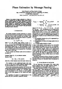
type of phase diversity. The goal is to identify a combination of object and aberrations that is consistent with all the collected images, given the known phase diversities. The phase-diversity technique offers several advantages over other aberration-sensing methods. The optical hardware required is modest. For example, a simple beam splitter and a second detector array will permit the simultaneous collection of the two images, as illustrated in Fig. 1. In addition, the method relies heavily on an external reference: the object being imaged. Therefore the method is less susceptible to systematic errors introduced by optical hardware. The technique also works well for extended objects. Finally, each photon is used for both imaging and aberration estimation. This may be preferable to the strategy of diverting valuable photons from the imagery to a separate wave-front sensor, where they are used solely for aberration estimation. The use of phase diversity to infer aberrations when imaging incoherently illuminated, extended objects was proposed by Gonsalves.5', Gonsalves derived an objective function for the estimation of aberration parameters that requires two collected images but does not explicitly depend on an object estimate. Conventional nonlinear optimization has been applied to this objective function in simulation experiments that resulted in the accurate estimation of aberration parameters. 6 -8 Once these estimates are known, an estimate of the system optical transfer function (OTF) can be constructed, and the object can be restored by using, for example, Wiener filtering. Simulation studies have also been performed to investigate the sensitivity of the phase-diversity method to additive noise and to certain systematic errors.8 The ability to operate on image subframes successfully, which is a fundamental requirement in the application of phase diversity to scenes, has also been demonstrated. 8 In this paper we examine the phase-diversity technique from the viewpoint of maximum-likelihood estimation. We also generalize the technique to accommodate an arbitrary number of diversity measurements. In Section 2 we pose the problem of jointly estimating the object and aberC)1992 Optical Society of America

maVol. 9, No. 7/July 1992/J. Opt. Soc. Am. A

Paxman et al. aberrated

Diversity is introduced by including a known phase function in the generalized pupil function of the system:

optical

system __

beam conventional splitter image

(It %

N

--

Hk (u) = Hk (U)Iexp{i[O(U) +

})fknown

a=~~~ defocus

diversity image,

length

Fig. 1. Optical layout of a phase-diversity system. The conventional image is degraded by aberrations in the optical system. The diversity image is degraded by the combination of the same aberrations and a known amount of defocus.

rations from diversity data. This problem is considered under an additive Gaussian noise model in Section 3. We derive an objective function that does not depend explicitly on the object and that yields the maximum-likelihood

estimate (MLE) for the aberration parameters when maximized. This objective function is shown to be a generalization of the Gonsalves objective function. An expression for the gradient of this objective function is also derived. The computational burden incurred in evaluating this gradient expression is surprisingly light. In Section 4 the same problem is considered under a Poisson (photon-limited) noise model. In this case an objective function that does not depend explicitly on the object has not been found. However, an expression for the gradient of the log-likelihood function is derived and found to be computationally tractable. This suggests the use of a gradient-search technique to maximize the log-likelihood function over the set of object pixels and aberration parameters. The gradient of the log likelihood is also given for the special case in which the object is known a priori to be pointlike. Finally, we construct an expectationmaximization (EM) algorithm for the joint estimation of an object and the aberrations. One advantage of this iterative algorithm is that object estimates are constrained to be nonnegative in a natural fashion. 2.

Frequently, space-invariant incoherent imagery is formed continuously through a convolution operation and detected discretely with a detector array. The analysis for our problem simplifies, however, if we model the object and its Fourier transform as discrete arrays. Accordingly, the incoherent image-formation process is approximated by the following discrete and cyclic convolution: =

E f(x )Sk(X - X')

(1)

x'EX

-f * S(X),

(2)

where f is the object array, sk is a PSF having diversity k, gk is the kth diversity image, and x is a two-dimensional coordinate. We treat the object, the PSF's, and the images as periodic arrays with a period cell of size N x N. These arrays are completely specified by their functional values on the set X,where

X = {0,1,...,N - 1} x {0,1,...,N - 1}.

Ok (U)]},

(4)

where is the unknown phase-aberration function that we would like to estimate, ok is a known phase function associated with the kth diversity image, and u E X. Phase diversity can be created, for example, by intentionally defocusing the system by known amounts. Note that in general each binary pupil mask H I could also change with the differing diversity measurements. It is often convenient to parameterize the unknown phase-aberration function:

+(u)= E. ajoj(u), j=1

(5)

where J coefficients in the set {aj} serve as parameters and {y} is a convenient set of basis functions, such as discretized Zernike polynomials for a monolithic aperture or piston and tilt basis functions, used to represent misalignments in a phased-array system. The form and the number of basis functions employed will depend on the nature of the aberrations involved. However, there is no loss of generality in parameterizing the phase function since the parameters could represent the point-by-point phase values, in which case the basis functions will be Kronecker delta functions: 0j(U) = 8U"j-{I

U = Uj

Ui-0 u snU

(6)

For notational convenience we construct a J-dimensional aberration parameter vector a with elementsal, a 2 , .. ., aj. The inverse discrete Fourier transform of the generalized pupil function gives the impulse-response function for a coherently illuminated object: hk

(x)

=

1

7

Hk(u)exp(i27r(u,x)/N),

(7)

where ( , )represents an inner product. The incoherent PSF is just the squared modulus of the coherent impulseresponse function:

STATEMENT OF PROBLEM

gk(X)

1073

Sk (X) =

hk (X) 2 .

(8)

The PSF depends on the aberration parameters through Eqs. (4), (5), (7), and (8). The noiseless image gk depends, in turn, on the PSF through Eq. (1). Of course any detected imagery will contain noise. The relationship between a noiseless image and the actual detected image dk will depend on the specific noise mechanisms. The problem that we address may now be stated. Given the set of K detected diversity images {dk},the corresponding set of phase-diversity functions {Ok}, and the binary pupil functions {JHkJ},estimate the object f and the aberration parameters a. Weconsider this problem in the cases for which the noise is modeled as additive Gaussian and Poisson.

3. ADDITIVE GAUSSIAN NOISE CASE We now consider the case in which the noise at each detector element is modeled as an additive, independent, and

1074

Paxman et al.

J. Opt. Soc. Am. A/Vol. 9, No. 7/July 1992

identically distributed random variable with a zero-mean Gaussian probability density having a variance 0r 2. Such a model would be appropriate, for example, if the dominant noise were thermal noise. In this case each detected diversity image dk is related to the corresponding noiseless diversity image gk as follows:

d*(x) = g(X) + nk(x)

(10)

where nk represents the additive noise. Note that, because of the noise component, dk(x) will be a random variable with a normal probability density: exp{

= (2o -)2

nificant reduction in the dimension of the parameter space over which a numerical optimization is performed. This approach is made possible by the existence of a closed-form expression for the object that maximizes the log-likelihood function, given a fixed aberration function:

(9)

=f * S(x) + nk(X),

W; fdk a]

depends explicitly on the aberration parameters but only implicitly on the object pixel values.5 The result is a sig-

[dk(x)- f * Sk(X)]l 2

(

FM(u)=

D1(u)S*(u) + D 2 (u)S 2 *(u) 2 IS1(u) 2 + S2(U)1

(15)

where an asterisk used as a superscript implies complex conjugation. Substituting this expression into the loglikelihood function [Eq. (14)] and dropping the 1/N2 scale factor yields a new objective function that does not depend explicitly on an object estimate:

(11)

The probability density for realizing an entire data l set {d*},consisting of all the pixels in each detected dive]'sity image, is given by K

p({dk};

a)

=

HI 1r Xexp

1 2)1/2

[#d(X)- f * S(X)]2}

exp~~~

20'n2

(12)

The MLE is the estimate that is most likely to Iiave produced a specific measurement.9 It is found by nt a mizing the likelihood function [Eq. (12) evaluated wi Tha

specific measurement] with respect to f and a.

The maximization is more easily carried out on a modified loglikelihood function:

L(f,a)=

K

-I k-1

2 [dk(x)- f

(13)

* Sk(X)]

XEX

LM(a)Lm = _>2, ID1(U)S 2 2 2 (U)2 -+ DS(u1 2 (U)S1(U) u) XIS,,(U)1

where it has been assumed that Sl(u) and S 2(u) do not simultaneously go to zero for u E X. It is important to recognize that maximizing the Gonsalves objective function LMyields the MLE for the aberration parameters explicitly and the object parameters implicitly, under the additive Gaussian noise model. Note that the dimension of the parameter space over which a numerical optimization is performed is dramatically reduced, since the N x N object parameters have been eliminated. Figure 2 illustrates how a two-dimensional log-likelihood function would be mapped into a one-dimensional objective function by this method. Let the X axis represent an aberration parameter and the Y axis represent an object parameter. The contour plot represents the log-likelihood function L, and the goal is to find the coordinates of the peak value. The locus of points (X, YM), for which YM maximizes L given X, traces out a curved line that corre-

which is obtained by taking the natural logarithm offthe likelihood function and dropping an inconsequential constant term and scale factor. For convenience we reft er to L as the log-likelihood function. Applying discrete versions of both Parseval's theorem and the convolution t heo-

Y (object parameter) ridge

reml' to Eq. (13), we have that

L(f a) =-

1

K

2K N 2k-1

-X 2

IDk(u)- F(u)Sk(u)1 ,

uEX

(16)

(aberration\ parameter)

(14)

where Dk, F, and Sk are discrete Fourier transforms of da, f, and S, respectively. Recall that Sk has the role of an unnormalized OTE"1 Note that maximizing the loglikelihood function is equivalent to minimizing the sum of squared differences, which is the error metric used by Gonsalves. The application of nonlinear optimization techniques to the log-likelihood function could be used to estimate the object and aberration functions simultaneously. This would require searching over a parameter space of large dimension, with object pixel values and aberration parameters serving as the axes of the space. Gonsalves showed, for the case of K = 2, that the aberration parameters can

be estimated by optimizing an objective function that

objective function 'evaluatedalong ridge

I

~~~X aberration (parameter)

Fig. 2. Pictorial representation of the construction of the aberration-only objective function. The two-dimensional contour plot represents the log-likelihood function. A ridge of the contour plot is defined by the locus of points (X, YM) for which YM

maximizes L for each value of X. The projection of the ridge values in the Y direction yields the one-dimensional, aberrationonly objective function.

Paxman et al.

Vol. 9, No. 7/July 1992/J. Opt. Soc. Am. A

sponds to a ridge in the contour plot. Substitution of a closed-form expression for Y into the expression for L maps the objective-function values along the ridge into a function of X alone. The resulting one-dimensional function is analogous to the Gonsalves objective function. The maximum of this objective function, corresponding to the MLE of the aberration parameter, can then be independently pursued. Once this MLE for the aberration parameter is found, it can be used in the closed-form expression for YMto find the MLE for the object parameter. We now proceed to generalize the Gonsalves objective function to accommodate an arbitrary number K of diversity measurements. We seek an expression for the particular F that maximizes L, given in Eq. (14). The real and imaginary parts of any such FMwill satisfy the following equations:

simultaneously go to zero at selected spatial frequencies. An alternative form for Eq. (20), also derived in Appendix B, is K

2

LM(a) =

FM(U)=

u E X1 E Xo

,

(19)

1

(21)

.

to

)Dk* -( Di Sk*

1

S112)

u E X1

u E Xo

K

JDj(u)Sk(u)- Dk(u)Sj(u)

kk)(U) (22)

where

i

where the set of spatial frequencies Xhas been partitioned into the subset Xo,the set of spatial frequencies at which all the OTF's are zero valued, and its complement, X1. Equation (19) indicates that, when u E Xo,FMcan take on any complex value so long as the Hermitian property of F or, equivalently, the real-valued property of f is satisfied. Any of the set of functions defined by Eq. (19) is a maximum-likelihood object estimate for a fixed aberration function. When a single solution is required, additional constraints must be imposed. For example, the minimum-norm solution is found by setting FM= 0 for u E Xo. This estimate has been proposed for use in selfreferenced speckle holography. 2 -4 In Appendix B we show that substituting any one of the estimates defined by Eq. (19) into Eq. (14) and dropping the 1/N2 scale factor yields a generalized objective function,

UeXi

2

k1

- Lm = - 422j 0U)IM ( [ Hk(U)(Z*k* aa,, N rx kk~4i

/K

Zk(U) = - 0

j=1 k=j+1

uEx

Many of these techniques repeatedly compute the gradient of the objective function. An analytic expression for the partial derivative of the objective function with respect to the aberration parameters, given a mild assumption on the OTF's, is derived in Appendix C and is given by

(18)

I JS112 EDj Sj*

LM(a)= - E

: IDk(u)

-

find aberration parameters that maximize Eq. (21).

u

K-1

2

term of Eq. (20) is an iterated summation. We may employ nonlinear optimization techniques'

u E X,

ISI(u)12 1=1

IS,(U)1

single summation, whereas the numerator in the first

where Fr(U)and Fi(u) are the real and the imaginary parts of F(u), respectively. The solution for Eqs. (17) and (18) is derived in Appendix A and is given by K E Dk(u)Sk*(U) k-1

K

>

K

This alternative expression is preferable to Eq. (20) since its evaluation requires fewer operations. The second term in Eq. (21) is just a constant, independent of the estimated aberration parameters. As a result, only the first term needs to be computed during the optimization sequence. Furthermore, the numerator of the first term contains a

aFr(u)( OFi (u)

j

2

Dj(u)Sj*(u)

1=1

a~ O(17) L= 0

1075

2

K 2 E ISI(U)1 L=1

* (23)

In these equations the operator Im[-] takes the imaginary part of the argument, and the summations overj, k, and 1 run from 1 to K. Equation (22) is exact and is therefore preferable to approximations provided by the method of finite differences. Moreover, using this analytic gradient can provide a significant computational savings over such approximations. Note that the argument of the operator taking the imaginary part is the same for all aberration parameters. Therefore this argument needs to be computed only once for a full gradient computation. The computation of the gradient, through the use of Eq. (22), will be dominated by the 4K fast Fourier transforms (FFT's) required (2K to construct the Sk and 2K for the convolutions), where K is the number of diversity measurements. By comparison, 2K(J + 1) FFT's are required to approximate the gradient by using the method of onesided finite differences, where J is the number of aberration parameters. We now consider the form of the gradient in two special cases. For the important case of K = 2, Eq. (22) reduces to

K -E

2 Z IDk(u)1 .

(20)

uEXOk1

Note that this expression agrees with Eq. (16) when K = 2. Furthermore, LM is now well defined even if the OTF's

-LM aaC,

=

42

N

4(U)ImEH1(U)(ZS 2 * H,*)(U)

uE*X

- H2(U)(ZS * H2*)(U)],

(24)

1076

Paxmanet al.

J. Opt. Soc. Am. A/Vol. 9, No. 7/July 1992

where

I(DSl*

the object and aberration parameters is

+ D2 S2*)(D2*Sl* - D*S 2*)

Z(U) 9 io

(IS,1

2

K

L(f e) =

u E X1

+ 1S2 1 )

u E Xo (25)

E [dk(x) >

4

Once an aberration function that maximizes LM is found, the corresponding OTF's can be constructed, and the MLE of the object is easily computed with Eq. (19).

)

(30)

= E E f(X) E Sk( - )

(31)

= E E f(x') EIh(x

(32)

k-1 x Ex K

=

exp[-gk(x)]

(27)

We assume that the number of photoevents realized will be statistically independent for each pixel. Therefore the probability of realizing an entire data set {dk} will be K ({ })d g(X)kx

x,)12

X

E

J~k(u)exp - i27r(u,x')/N)

12

(33)

uEX

1

K

>,f(x') N k> uX > jHk() 2, XEx

=

(34)

where we have used discrete versions of the Fourier shift theorem and Parseval's theorem.'0 Note that the double sum over the squared moduli of the pupil functions is just a constant, independent of the object, the aberration parameters, and the phase diversity. Let K

C-

2 IlHk(U)12 .

2

(35)

Equation (34) then becomes K

= CE

2 Z gk (

k=i xEX

xEX

f(x),

(36)

and the log-likelihood function simplifies to K

dk(x)lng(x)

L(f, ) =

-

k=i xEX

C 2 f(x)

_

K

(37)

xEx

_

2 dk(x)ln 2

f(x')sk(x -

) - C>2f(x).

x'EX

xEX

(38)

We now consider the case in which the data are limited by photon noise. In this case the number of photoconversions that occur at each detector element will be a Poissondistributed random variable with a mean value prescribed by the noiseless image gk given in units of mean detected photons per pixel. Therefore the probability of detecting dk photoevents at location x is

Pr({dk}) = H H

-

xE AXP) 2

k=l xEX

gk(x)k()

xEX 1

k-l xEy

POISSON NOISE CASE

Pr[dk(x)] =

xEX

k=l xEx K

=2 4.

E f(X )Sk( -

k- xX x EX K

k=1 xEX

Hk(U)(Zk * Hk*)(un) (26)

Note that the number of FFT's required for computing the gradient in this case is the same as that when the aberration basis functions are polynomials. However, the projection onto all J basis functions is not needed here. Hence the point-by-point phase gradient is somewhat easier to compute. Using simulation experiments, we have observed that, when Gaussian noise is added to the imagery, the objective function LM takes on a rough texture containing many local maxima.7 The nalve application of gradient-search methods to this objective function will result in rapid entrapment by a local maximum. One strategy for handling this problem is to use an algorithm, such as simulated annealing, that is designed to find a global maximum in the presence of local maxima. Alternatively, regularization techniques can be used to smooth the objective function so that a gradient-search algorithm would yield a regularized MLE. We have had preliminary experience with two regularization strategies, and in both cases appropriately modifying the closed-form expression for the gradient has been straightforward.

(29)

K

gk(x) = E, I

E

[MK

-Lm= -- i

gk(x)],

-

where an inconsequential constant has been dropped. Consider the second term in Eq. (29): K

A second special case arises when we are trying to estimate the point-by-point phase values in the generalized pupil function. In this case the aberration basis functions will be Kronecker delta functions 5,u., and Eq. (22) reduces to

ln g(x)

k=1 xEX

22

exp[-gk(x)]

At this point we could logically follow the same strategy that we pursued in the Gaussian noise case in an effort to reduce the dimension of the parameter space over which a numerical optimization is performed. The desired sequence is to solve for the MLE of the object, given fixed aberration parameters, and substitute this result into the expression for the log-likelihood function to create an objective function that does not depend explicitly on the object estimate. We begin by computing the partial derivative of the log-likelihood function with respect to the ith pixel value of the object estimate: a=K

af(xi)

2

2

k=l

xEX

(28)

dk(x)

a af(xi)

ln

x'Ex

f(x')sk(x

-

) (39)

XEXaf(xi)

It-i1 xXydx)

K

A modified log-likelihood function (henceforth referred to as the log-likelihood function) for the joint estimation of 'i,

dk(x)sk(x - Xi) - C

k-lXEX 2 f(x')sk(x x'ex

x)

(40)

To find the MLE of the object for fixed aberration parameters we set this partial derivative equal to zero and

The log-likelihood function can be modified to accommodate faulty detector elements:

attempt to solve for f:

K

L (, ) dk(X)sk(X

K

- Xi)

eX

>2

C.

x'CX

Solving Eq. (41) would provide the MLE of the object for

the multiple-kernel deconvolution problem given Poisson noise. The same problem is encountered in time-of-flight positron emission topography.'6 Unfortunately, a closedform solution for f has not been found, and hope for the derivation of an aberration-only objective function is diminished. Note, however, that the partial derivative with

is readily shown to be

a af(xi)

The tractability of the computation implied by Eq. (40) suggests the use of a gradient-search technique in maximizing the log-likelihood function over object pixels and aberration parameters simultaneously. Recall that the complete gradient also requires partial derivatives of the log-likelihood function with respect to the aberration parameters. The expression for these partial derivatives is derived in Appendix D and is given here as

aa,

FK

uEX

k l

X(exp(i2 (

')/N)2 EX

1

N

2E

.,.x

h*(x')

dk(x) fX

>Ef(x")Sk(X

x')

-

-

X")

1

(42)

x"E-X

K

L.= -2 E aan

derivatives {aL/aan} is reasonable and does not de-

pend on the number of parameters J Because there is significant overlap in the computation of aL/af(xi) and aL/aa, the total number of FFT's required for computation of the gradient of the log-likelihood function is only 7K + 1. Having derived expressions for the partial derivatives of the log-likelihood function with respect to object pixels and aberration parameters, we are now in a position to suggest a strategy for the joint estimation of object and aberration parameters. These partial derivatives constitute a gradient of the log-likelihood function in a parameter space of dimension N X N X J The computation of this analytic gradient requires multiple FFT's but is manageable, unlike a finite-difference computation. Any of a variety of unconstrained and constrained nonlinear optimization algorithms that utilize the gradient can be employed to search iteratively for a global maximum.' 5 Constrained optimization methods allow us to enforce the nonnegativity property of incoherently illuminated objects in our estimate. Perhaps a good initial estimate would be the solution under the Gaussian noise model. If it can be found, the global maximum will provide the MLE for both the object pixel values and the aberration parameters.

1

-

Wk(X)Sk(X

(44)

Xi).

-

K

n(U)Im 2 Hk(U) k-1

uEx

X exp(i2T(u, x')/N)>2[dk(X)

-

22E

N

h*(x')

.'Ex

1]WkXvfX

-

(45)

X9}.

It is also worth considering the special case in which the object is known a priori to be unresolved or pointlike. This case has been important to researchers seeking to estimate the aberrations present in the Hubble Space Telescope from Hubble images of stars.3 4 When the point-object assumption is valid, the object is known, and there remain only aberration parameters to estimate. It is straightforward to show that the log-likelihood function is insensitive to shifts in object position. Therefore there is no loss of generality in modeling the point object as a weighted Kronecker delta located at the origin:

Careful scrutiny of Eq. (42) shows that the number of FFT's (6K + 1) required for computing the entire set of partial

[dk(x)

kx >2 >2k LgA

Similarly, the partial derivative with respect to the nth abberation parameter is found to be

Gradient-Search Algorithms

n(U)Im[ Hk(u)

(43)

where Wk is a binary window function with a value of unity for the detector elements that are functioning and zero for those that are faulty, in the kth detector array. This consideration would be important, for example, when phase-diversity methods are applied to the Hubble phaseestimation problem, for which selected detector elements are known to have failed. The partial derivative of this log-likelihood function with respect to the ith pixel value

respect to each object pixel [Eq. (40)] can be found for all

object pixels with a reasonable number of FFT's (3K + 1 FFT's, assuming that the OTF's are precomputed). This computation would be unmanageable if the method of finite differences were used.

= -22

[dk(x)ln g (X) - g(X)] Wk(X)

(41)

X')

-

f(x')Sk(X

= 2 2 k=1 xEX

k=1

a -L

1077

Vol. 9, No. 7/July 1992/J. Opt. Soc. Am. A

Paxman et al.

f(x) = a8(x),

(46)

where ^ {1

x = (0,0)

0

otherwise

(7

Given this model, Eq. (42) quickly simplifies to

a

FK

-L aan

2 _n(tU)ImL

Hk(u)

N

k=1

UCX

1

> x'EX

hk*(xI)dk(XI)

s(x')

Sk(X )

(48)

X exp(i2iT(u, X')/N)]*

If we define 1

___________X~

N2

Lhk*xdk(X)

E

hk*(x)dk(x) Sk(X)

exp(i2T(u,

x)/N), (49)

then Eq. (48) assumes the succinct form

L = -22 aa,,

uEX

T

f(U)IM E Hk(u)9;u k=1

11]3 S(X)

(50)

1078

J. Opt. Soc. Am. A/Vol. 9, No. 7/July 1992

Paxmanet al.

This expression gives the partial derivative of the loglikelihood function with respect to aberration parameters for a point object given multiple diversity images corrupted by Poisson noise. A gradient evaluation requires only 2K FFT's, again suggesting the use of a gradient-search algorithm. Care must be used when invoking the pointobject assumption. For example, if this assumption were unwittingly applied to images of a binary star, the resulting aberration estimates could be significantly biased. Expectation-Maximization

Algorithm

In this section we construct an EM algorithm as an alternative means to find the MLE of the object and aberrations in the case of Poisson noise. The use of an EM algorithm is suggested by similarities between our problem and time-of-flight positron emission tomography, in which EM algorithms have been applied with considerable success. 6,7 Kaufman has shown that there is a close relationship between the EM algorithm used in positron

emission tomography and gradient-search methods.8

One potential advantage of the proposed EM algorithm over a constrained gradient-search algorithm is that the nonnegativity constraint is enforced in a natural fashion. The EM algorithm is iterative, producing a sequence of estimates of the object and aberration parameters with the property that the log likelihood of these estimates is a nondecreasing function of the iteration number. General descriptions of the EM algorithm and its convergence properties are found in Refs. 19 and 20. The derivation of our EM algorithm begins with the construction of an abstract statistical model. Recall that the measured data dk(x) indexed by k and x consist of independent Poisson random variables, each with the expected value

dk(x)= E dk(x x') -

Using terminology associated with the EM algorithm, we refer to the random variables dk(x x') as the complete data and the actual collected data dk(x) as the incomplete data. The choice of the abstract data set dk(x I x') as the complete data is somewhat arbitrary, and other choices could lead to alternative algorithms. The EM algorithm is a prescription for updating the set of parameter estimates {f (r),a (r)}to the new set of parameter estimates {f(r+), (r+l)} having the property that

L[f (" a

K

L~d(f,a)

2E {ak(XXI)

2

X ln[f(x')Sk(X

(52)

This expected value can be interpreted as the mean number of photons detected at pixel x, originating from the object at pixel x'. Any sum of the random variables dk(x I x') will produce a new random variable that is Poisson distributed with an expected value that is obtained by appropriately summing the gk(XIx'), as can be readily verified by using characteristic functions. For example, the random variables indexed by k and x,

(53)

2 ak(X4',

x'EX

will be independent and Poisson distributed, with expected values equal to

=

>2[> K

+ E 2 2

(xIx)ln

k-1 xEx x'EX K

-

X'EX

2

f(x')Sk(X

-

X')

Therefore a model that is statistically consistent with our measured data results from treating the collected data as

(59)

K

= x'ExL 2 k-1 2 XEX Ea(xlx') lnfx' K

(XIIx

2

k-l x'Ex

Ca X

-

x') In

Sk(X )

K

- 2 f(x')22 sk(x), X'Ex

(60)

k-1 XEX

where inconsequential terms have been dropped. The expectation step (or E step) consists of evaluating the conditional expectation of Led, given the measured data dk and

assuming that the parameters governing the complete data are equal to is defined as

This conditional expectation

{f(r), a(r)}.

Q[t a f(r) a(r)]

E(r)[Lcd(, CZ)I {d}],

(61)

where E(r)[.]denotes an expectation in which the parameters associated with the complete data take on the values {f(r) a(r)}. The maximization step (or M step) of the EM algorithm consists of assigning to {f(r+l), a (r+i)} the values of {f,a} that maximize Q subject to any constraints that may exist. As derived in Appendix E, the resulting iterations are f(r+l)(X,) = f(rx)

2 >

K

Sk(r)(X

-

X) dk()

(

(62)

xGX

k-1

(54) (56)

X')

k-i XEX

K

X'Ex

-gi,(X).

Sk(X -

f(x')>22 Sk(X- x')

2

x'Gx

k-1

X') =

f(x')sk(x - x)} (58)

I x') n f(x')

>2d*xk x'EX k=1 xEX

>2Sk(O)

E Rk (XI

X')] -

-

K

x'Ex

gk(XI X ) = f(x')Sk(X - X') .

(57)

k-i xEx x'EX

(51)

Now consider a collection of random variables dk(x I x') indexed by k, x, and x', and let them be independent Poissondistributed random variables, each with the expected value

---L[f `) a W] ,

r+l)]

where the superscripts in parentheses represent the iteration numbers. The prescription requires an expression for the (modified) log-likelihood function associated with the complete data Ld. For our problem this expression is found [by analogy with Eq. (29)] to be

+ E

gk(X) = 2 f(X')Sk(X x

(56)

x'Ex

a(r+l) = arg max a

X

[

E 1 1k-i x'Ex

f(r)(X

Xt)S(r)(W ) dk(x)

ln Sk(X')J ,

(63)

where gk'r)(X) Sk(r)

>2 fk(r)(x)sk(r)(x - x x'EX

(64)

,

kth diversity PSF evaluated for a(r)

(65) (66)

Sk(0) = 2 Sk(X) XEX

Note that Sk (0) is independent of the particular aberration parameters. In the iterations zero divided by zero is defined to be zero. Since the likelihood is a nondecreasing function of r, when it is properly initialized the algorithm will never produce gk(r)(x) = 0 when dk(x) $ 0. Whereas Eq. (62) presents a closed-form expression for

updating the object parameter estimates, Eq. (63) requires the solution to an optimization problem in order to update

the aberration-parameter estimates. Fortunately, this optimization occurs in a space with a relatively small dimension, the space of aberration parameters. Moreover, a closed-form expression for the gradient of the argument to be maximized in Eq. (63) is available for use in the optimization sequence. This gradient expression is analogous to that derived for the point-object case, as is discussed in Appendix E. We conclude this discussion of the EM algorithm by considering its application in two special cases. One special case arises when the phase-aberration parameters are known a priori. In this case the EM algorithm for estimating the object intensity is

f~rl)(,) f~)( (f (XP)

f~r~i(xI)

K ___K

1 _

K 2 Sk(X >2

k__ 1 xEX

-

X

)dk (X)X ) 9k(r)

_X

(67)

>2Sk (O) k1XXg~~

MAXIMUM-LIKELIHOOD

APPENDIX A:

OBJECT ESTIMATE

FOR THE GAUSSIAN

CASE In this appendix we derive the expression for the MLE of the object under the additive Gaussian noise model and Recall that the logfor fixed aberration parameters. likelihood function is given by K2

which is essentially the same as the EM algorithm derived by Snyder and Politte'5 and Politte' 7 for time-of-flight positron emission tomography. For this case, arguments similar to those used by Vardi et al.2 ' can be used to show that f(r) converges to a global maximum

gradient of this aberration-only objective function that will allow for an efficient gradient-search phase-estimation algorithm was derived. An expression for the log-likelihood function has been presented for the Poisson noise case as well. An attempt to derive an aberration-only objective function by analogy with the Gaussian noise case failed. However, an analytic expression for the gradient of the log-likelihood function was derived and shown to be computationally tractable, suggesting the use of a gradient-search algorithm. An EM algorithm that incorporates a nonnegativity constraint in a natural fashion was also presented. The viability of the phase-diversity concept was previously demonstrated through computer simulation for the case of Gaussian noise with K = 2.` In the case of Poisson noise, the gradient-search and EM algorithms described herein need to be exercised to demonstrate their utility. In every case additional simulations and theory are needed to quantify the performance of the estimates as a function of the number of diversity images, the types of diversity, and the level of noise. A particularly intriguing issue is the optimum distribution of a fixed number of photons among diversity images.

L(f,a)

k=1

=

cial case arises when the object is known to be a point

source. In this case the EM algorithm for estimating the unknown aberration parameters will converge in one iteration to the maximum-likelihood solution.

a L= 0,

(Al)

(A2)

aFr(u)

u E X,

aFi(u) =

(A3)

where Fr(u) and Fi(u) are the real and the imaginary parts of F(u), respectively. Consider the partial derivative of L with respect to Fr(u):

a L= - 12K

a(IDk 12 + kI k-Z 1

aFr

IFSkl'

- DkF*Sk* - Dk*FSk)

SUMMARY

We have formally stated the problem of the joint estimation of the object and aberrations by using phase diversity. Maximum-likelihood estimation has been considered under Gaussian and Poisson noise models. In the Gaussian noise case the estimation of the aberration parameters can be accomplished without explicitly estimating the object pixel values. An aberration-only objective function, first derived by Gonsalves, was shown to yield a maximumlikelihood estimate, and this objective function was generalized to accommodate an arbitrary number of diversity measurements. Moreover, an analytic expression for the

IDk(u') - F(u')Sk(u')l.

Nh -X2

We seek an expression for F(u) that maximizes L. Stationary points of L are achieved when

of the log likeli-

hood. Under certain assumptions about the PSF's, {Sk}, this solution can be shown to be unique. With the additional restriction that K = 1, the iterative rule in Eq. (67) is the same as that independently derived by Richardson2 2 and Lucy,2 using a Bayesian viewpoint. The second spe-

5.

1079

Vol. 9, No. 7/July 1992/J. Opt. Soc. Am. A

Paxman et al.

[ Sk

=

a (Fr2+ Fe2)-

DkSk

(A4)

Dk*Sk] (A5)

1

-RN2

K

(21SklFFr

Dk Sk - D*Sk)

,

(A6)

where we have suppressed the dependence on u for brevity. Similarly, a

= L= - ~~ (2ISkI2'Fi + iD,Sk* -

iDk*Sk).-

(A)

1080

J. Opt. Soc. Am. A/Vol. 9, No. 7/July 1992

Paxman et al.

We now set the right-hand side of Eq. (A6) equal to zero

By examining the second-order partial derivatives of L with respect to the real and imaginary parts of F at each spatial frequency, one can show that L is a concave function.5 As a consequence, Eq. (A15) represents the set of objects that globally maximize L and therefore defines the set of maximum-likelihood object estimates.

and solve for Fr: K

K

k-1

k-i

2 2Fr 2 Sk1 = 2 (DkSk* + Dk*Sk),

K

/ K

E (DkSk* + Fr(u) =

(A8) E IS1 12

Dk*Sk)2

-)

U E X1

1=1 u

APPENDIX B:

(A9)

Substitution of any of the maximum-likelihood object estimates into the log-likelihood function and eliminating the 1/N2 scale factor yields a new objective function LM(a) for the estimation of the aberrations. The derivation of this new objective function is presented here:

where we have partitioned the set of spatial frequen into the subset Xo,the set of spatial frequencies at all the OTF's are zero valued, and its complemen Formally,

K

Xo = {u Sk(U) = 0, k = 1,...,K}, X = {u:U E

(A10)

LM(a) = ->E E Dh(u) uE kl

U Xo}-

=-EuEX1>k Dk

U E X,

FM(u)= Fr(u)+ iFi(u) / K

[DkSk* + D*Sk + iDkSk*i

+ Dk*Ski)] 22

ISI2

-

E

E

Dk,

(B2)

uE:X k

u E

Fm*(-u)

u E yX

(A14)

/

K

k

2 >2 IS4

(A13)

K

E

2

S

however, in the event that the OTF's simultaneously go to zero at spatial frequencies within the union of diffractionlimited OTF supports. We now focus our attention on the first term in Eq. (B2), which we designate by LMi. Expanding this term, we have that

Eqs. (A9) and (A12) as follows:

=

-

(B1)

tion. Strictly speaking, this term must be retained,

u E Xo

The set of stationary points of L is found by combining

{

FM(U)Sk(U)2

where the u dependence has been suppressed and the summations over j, k, and I run from 1 to K. Equation (B2) consists of two major terms distinguished by the summations over X1and Xo. Recall that Xois the set of spatial frequencies at which all the OTF's are zero valued and Xi is the complement of Xo. Note that the values of FM at spatial frequencies in Xoare irrelevant since Sk(u) is zero there. Also note that the contribution to the second term in Eq. (B2) from data at spatial frequencies outside the union of diffraction-limited OTF supports will be constant and will not affect the contour of the objective func-

/ K

E (-Dk Sk* + Dk*Sk)i 2>S 1 2 Fi(u) = k-U 1=1

-

>2p$*

The set Xo includes all spatial frequencies that fall outside the union of the supports of all K diffraction-limited OTF's, that is, all the spatial frequencies beyond the system diffraction-limited cutoff. Note that it also includes any spatial frequencies interior to this union of supports for which the OFT's simultaneously go to zero owing to aberrations. Equation (A9) indicates that, when u e Xo, Fr(u) can take on any complex value so long as F(u) = F(-u), which is consistent with the Hermitian property of F or, equivalently, the real-valued property of f Setting the right-hand side of Eq. (A7) equal to zero, we get K

ABERRATION-ONLY

OBJECTIVE FUNCTION FOR THE GAUSSIAN CASE

E Xo

Ds*/

|SI|2

u / 1=1 FM*(-U)

u

G

X

(A15)

U E X°

Dk>2

LM=-E 2

1

2+

2 IS1

1J

uEx k 'I

_Sk>2Dj

I

Z JS112 D 1 Is2 2

Dk>2S1I

=UEX

E k

I

S*I2

(B3)

I

Sk>DjSl* j

2

-

Dk*>ZISl 2S Z DjSj* I

I

(2

IS V) 1

IE S112

-

ISI 2S* IDj*Sj

D I

Ji

- (B4)

Vol. 9, No. 7/July 1992/J. Opt. Soc. Am. A

Paxman et al.

Note that the summation over k affects only the numerator in Eq. (B4). We now distribute the k summation

over

each term in the numerator to get

2

I

k

IS,12) + E ISkI

j

k

I

2 ID(U)I2

LM(O)= -2

> IDk(U)12

-

(B5)

2

K

Sil) I 2 Z S22 ID12

2DE Ss* >

-

(B12)

uEXo k=i

j 2

2 IS1U)l

K

- >2DkSk*2I SI >EDj*Sj I

2

1=1

2

f-

_

SDjSj* j

k

j2 Dj(u)Sj (U)

K

DjSj*

uEX1 k=

- 2 Dk*SkhE >s 2 k

This expression retains the form of the Gonsalves objective function (K = 2) for direct comparison. An alternative form derives directly from Eq. (B7) and is given by

~~~~~~2

2

numerator = E IDk(

1081

2

=-2 (B6)

>2Dj(U)Sj*(U) K

uEX1

>2IS1(U) 2

K

>2

E IDh(U) 2 .

(B13)

uEXk=l

1=1

where the second and third terms in Eq. (B5) have been canceled. Factoring out the common factor yl IS,12 in the numerator and canceling this with the same factor in the we Let

denominator,

2

>2IDI2>2lSl2 - 2 >2DjSj* k i ES1

EX

B7) (B7)

S

uEXl

2 2 Dk Sj2 - E 2 DjSj*Dk*Sk =

j

k i

UE

L2 IS1 l

uEXl

k

(B8)

2

APPENDIX C: PARTIAL DERIVATIVE OF THE ABERRATION-ONLY OBJECTIVE FUNCTION FOR THE GAUSSIAN CASE In this appendix we derive an expression for the partial derivative of the objective function LMwith respect to an aberration parameter a,, for the case of additive Gaussian noise. Using the form of the objective function expressed in Eq. (21), we have that

d

a m => -LM aafn uExi aan

Ea Dj(U)Sj*(U)2

j=

K

E IS(U)

2

a -

K

aan uEx k=l

IDk(U)I2 .

1=1

(1/2)2 E

=

(C1)

>2ID Sj - Dj Sk 2

k i E IS11

(B9)

,

where we have used the fact that k and j are dummy indices. Note that the terms in the numerator for which

j = k vanish. Rearranging the summation limits to retain half the remaining terms in the numerator, we have that K-1

LMi = -

K

)j(U)Sk(U) - Dk(U)Sj(U)I 2

E

>2j=i

k=j+l

K

E ISi(U)I2

uEX1

1=1

Reintroducing the second term in the objective function gives K-1

K

1DJ(U)Sk(U) - Dk(U)Sj(U)1

LM(a)= - 2 j=l k=j+l

K

E ISl(U)12

UEXi

1=1

K

- >2>2IDk(u)2 . uEXO

k=l

2

The second term in Eq. (Cl) vanishes because the data are independent of the parameter estimates. The partial derivative in the first term is difficult to evaluate since the set Xi that defines the limits of the summation can actually depend on the aberration parameters. Indeed, the derivative may not exist at coordinates in the space of the aberration parameters for which the limits of summation are changing. To circumvent this problem we place a mild restriction on the set of OTF's. Consider the set of pixels Xs defined by the union of the diffraction-limited OTF supports. Spatial frequencies in the complement of Xs are permanent elements of Xoand never enter into the limits of summation in the first term in Eq. (Cl). It is only when the OTF's simultaneously go to zero at spatial frequencies within Xs that the limits of summation can vary as the aberrations change. Recall that the value of an OTF at a spatial frequency u E xs is the sum of unitlength phasors. Such a sum is unlikely to be exactly zero, particularly with random phases.2 4 The prospect of all K OTF's summing to zero at the same spatial frequency is even more remote. Therefore the limits of summation in Eq. (Cl) will be constant almost everywhere in the space of the aberration parameters. Weassume that the partial derivative is evaluated at the aberration parameters about which the OTF's do not simultaneously go to zero at spatial frequencies within Xs. When this is true, the partial derivative can be taken inside the summation as

1082

J. Opt. Soc. Am. A/Vol. 9, No. 7/July 1992 K

Paxman et al.

2

2 Dj(u)Sj*(u)

a -

-L = aCn

fleX,

aan

E

(C2)

SI(U)I 2

1-1

2 IS112 2 DjSj* 2 I

=

i

+c.c)-

Dk*Sk'

k

DjSj*92SI*SI' + c.c) (C3)

(E IS,12) I~~~~~~~~~ >2IslI2 2DDj *2 I

=

j

k

u~xJ

2

|2 Dj S*

Dk*Sk'-

>2 S*SI'

j

I

+ c.c.

(C4)

(ZIS112) E ZkSk' + c.c.,

=

(C5)

uEX k

where the u dependence has been suppressed; the summations overj, k, and I run from 1 to K; the prime applied to a function signifies a partial derivative; c.c. represents a term that is the complex conjugate of the preceding term; and we have defined

f[2

h

ISlI2(2,DJSj*)Dh* -

E2DjSj*Sk ]

(

where we have used the change of variables u" = u' - u in Eq. (C13).

Returning to the primary derivation, we substitute Eq. (C14) into Eq. (C5):

u E X1

52)2

u E Xo

Note that defining Zk in this way extends the summation in Eq. (C5) over all of X.

At this point we digress to derive an expression for the partial derivative of an OTF with respect to an aberration parameter. Recall that the unnormalized OTF for the kth diversity system is the discrete Fourier transform of the corresponding PSF:

Sk() = 2 k(x)exp(- i2 w(u,x)/N)

a

aa

-L = E

uex k=l

~K

i

-

~K

i

-2E N ',EX

>2K

(U) k-l Hk*(U) uGX e Zk(U)Hk(u' + U) + C.C.

(C8)

Equation (C8) can be rewritten in terms of the generalized pupil function H, using the discrete version of the autocorrelation theorem: Hk(U')Hk*(U'- u),

(C16)

Using the Hermitian property of Zk and the change of variables u" = -u' we rewrite the second term above as

secondterm =

(C9)

2E X I

( ) E Hk*(U)

Z*(-U)H(U'

+ U)

+ c.c.

(C17)

uEX

where

=Hk(U)

IHk(U)exp{i[

Ok + 2 ajkj(u)]}

(C10)

2 I Hk (uN 2 .,Cx[

U) a Hk(u ) + H aa"

)

a Hk*(U - U)]

aa"

L iOk(U)Hk(u')Hk*(U' i,,(u")Hk(U" + 2~~~~~~~~~~~~~~~~~

= (i/N2 )

-

> u'GX

N uEX

U EX

2 ) 2 [H*(u= (1/N u)i0.(u')Hk(u') - Hk(u)ip.(u - u)Hk*(U,- U)]

N2

i

~K

2 E 'O.(U ) E H*(U) k=l

x E Zh*(U)Hk(U - u )

The partial derivative of the OTF is

a Sk(U) aa,,

E o.(U,)

UX

N

,b k-i E Hk(U) uex 2 Zk(U)Hk*(u - u) + c.c. N 2u,ex O-(U')

(C7)

xC=X

Sk(U) = N2

f(U)i

X [H(u')H*(u' - U) - Hk*(U')Hk(U+ u)]} + c.c. (C15)

xEX

= xhC(X)12exp(-i2r(ux)IN). -

(C6)

n(U')[Hk(U)Hk*(U-

U) -

U) -

E

U)Hk*(U)]

Hk*(u')Hk(U'+ U)],

(Cll) (C12) (C13)

(C14)

+ c.c., (C18)

Vol. 9, No. 7/July 1992/J. Opt. Soc. Am. A

Paxman et al.

from which it is apparent that the second term is just the complex conjugate of the first term. Therefore

a

[2i Lm = [N X

Eq. (D2):

-Sh(X) = hk*(x) aa,,

HhU'

2

I On(U)

1083

+ c.c.

aan

(D3)

Hk(U)

2 Zk(U)Hk*(U ,EX

-

c.c.

U)] +

E Hk(u)exp(i2(U,

hk*(X) a 2

N

(C19)

aan

x)/N) + c.c.

uEx

(D4)

[~~K =4- 4(U,)IM

~~H)U] * k*)(u , >2'On( ')Im>2 Hk(U')(Zk

E

2h*(X) a

N2

aan

Hh(U)I

uEx

(C20)

X exp{i[Ok(U)+ a

(U)]}) (D5)

X exp(i2qr(u, x)/N) + c.c.

where the operator Im[-] takes the imaginary part of the argument.

=

in (u)H (u)exp(i2X(u, x)IN) + c.c.,

hk*(X)

APPENDIX D: PARTIAL DERIVATIVE WITH RESPECT TO ABERRATION PARAMETERS FOR THE POISSON CASE

(D6)

where c.c. represents a term that is the complex conjugate of the preceding term. Equation (D2) then becomes

In this appendix we derive the expression for the partial derivative of the log-likelihood function with respect to

a L=

~x)hh*(x [ -

dk(x) E k= xEx 9k W K

aan

[

k=l

2

i>n(u)Hk(u))

[K [ k= uEh

2

=-

x

2Z

h

)hh*(x -

ex2(- x2

WXxe,

(D7)

X)IN) + c.c.

(D8)

x')exp(i2T(u,x

h>*(x )exp(i27r(u, X)2U) '

1(Xf

N

+ c.c.

(D10)

] + C.C.

(Dll)

1

1-X'

(D12)

X )/IN) E

2 hk*(x')exp(i2,.(u, x')/N)>2

dk(X)f(x xex 2 f(X")S(X

x'E

c.c. (D9)

gk(x)

x

hk*(X )exp(i2r(u,

+

N)

-

x')hk*(x)exp(i27T(u,xx')]

x'EX

n.(u)Hk(u) N

= -22 En(U)Im[2KHk(U) uEX k=

x')/N) + c..]

2 i.()Hk(u)exp(i27r(ux -

x)

dhkx x'EX

N

-

uEX fN

>2f(x > g i n(u)Hk(U)XEX gk(X) x EX uEX

k-i ueX

= -

X

2

~~1 dk

K

2 Ki0.(u)Hk(U)N1

=

i,n(u)Hk(u)exp(i27r(u,x

uEX

x'Ex

dk()-Efx')/N)] =>2>2 >2 f(x') k=i xex gk(x) XEX

[,

')

>22f(X

-X)

(D13)

x

-

X")

-~~~~~~~~~~~X

aberration parameters for the case of Poisson noise. Recall that the log-likelihood function is given in Eq. (38). We now take the partial derivative,

K

- L=> >2 aan k=- xeX 2

a

dk(X) f(x")sh(x

-

>2 f(X') - Sh(X aan

X") x'ex

-

X')

where we have assumed that f is real valued in order to step from Eq. (D7) to Eq. (D8). Equation (D13) is the desired expression for the partial derivative of the loglikelihood function with respect to aberration parameters. APPENDIX E:

DERIVATION OF THE

EXPECTATION-MAXIMIZATION ALGORITHM FOR THE POISSON CASE

(Dl) K

dk(x)a

=> >2

E f(x')-sk(x - x), >2

kh- xex gk (x) X

aan

(D2)

where an is the nth parameter of the phase function 'k. Consider the partial derivative of the PSF, found in

In this appendix we derive an EM algorithm for the joint estimation of the object and aberrations in the case of Poisson noise. Recall that the E step of the EM algorithm requires the evaluation of the conditional expectation of the complete-data log likelihood: Q[f, a If('), a(')] = E(")[Lcd(f a) I{dk}],

(El)

1084

J. Opt. Soc. Am. A/Vol. 9, No. 7/July 1992

Paxman et al.

where E(`)E.]denotes an expectation assuming that the parameters governing the complete data take on the values {f(), a(')}. The log likelihood of the complete data was shown in Eq. (60) to be

where we have defined

EX [ki

=

x'CE

K

k

x'Ex

xE-X

+ 2

E2 Z d(x x -x)

k-1 x'Gx xex

(')(X)

ln sh(x)

Qa

=

k-i

(Ell)

k=1

E[

xEx

xEx

f~r)(

,)Sk )(X ) gr(X) dk

JIn

K

- E f(X') 2 E Sk(X). x'EX

ki xEX

E(r)[dh(X I x') I {dk}] = E(r)[d (X I X') I d(x)],

(E12)

Then f(r+i)is obtained by maximizing Qf, and a(r+) is obtained by maximizing Qf

K

(E4)

x'Ex

From Eq. (E4) we see that the expectation

-

(E5)

(Z1 + Z2)-

(X,)S(X

-

dk(x) (E13)

K E

1 [f(X,)] 2

-

f(r)(xt)s(r)(X g

X)

-

()()

_

dk(X)

0, (E14)

where 8(x) represents a Kronecker delta. global maximum

Ak2

X )

gx(X)

XEX

X')

af(x')af(x")

X

-

S0),

8X-

in Eq. (E3) is

Through the use of this rule and Eq. (52), the conditional expectation in Eq. (E3) is readily evaluated as

Therefore a

of Qf is found by setting Eq. (E13) to

zero. Consequently, we assign to f +') the values f(r+)(Xi)

= f(X)

>K, > Sh(r)(X - X )

K

>2Sk(O) hi

gk (X)

x~k

k =1

) dh(x),

(E6)

(E15)

Unfortunately, no closed-form expression is obvious for the maximizer of Qa, so we write

where s(X-x' k ( (r()= 9 >2 fh k r)x (X)Sk ) - X ,

(E7)

x'Ex

a (r~i)

Sh(r) kth diversity PSF evaluated for a(r). =

']

f'r),

=

L [K K

+ 2 I k-1

(X

- X)Sh W(XI)

dk(X)

EX

1

tk-i

k-1

K

(E9)

where S(O) = ExExSk(X) is independent of the aberration parameters. For the M step we determine the parameters {f a} that maximize Q subject to any constraints that

may exist and then assign the maximizing values to {f(r+l),a (r+i)}. Fortunately, this maximization may be performed separately over f and a.

d~)

1

(E16)

(E10)

E dh(x)lnS(X) >

k= xeX

+ C.

(E17)

Therefore we can use the closed-form expression for the gradient of the log-likelihood function in the point-object case in the optimization of Eq. (E16) by substituting dk(x)

-

->

x'e-x

We may rewrite Q as

Q[f, a f(r),a ] = Qf + Q.,

dk

(X')

L(a) =

Sk(0),

(r)( )

gh()~

X ln Sk(X')}-

gk

K

x'ex

a

[E fX X)W (In

r

- >2f(x')

E E f )( x'EX EX

arg max{ k

The optimization in Eq. (E16) bears a striking resemblance to the optimization of L(f a) when the object is known to be a point. In this special case Eq. (38) reduces to

fEr)(x ~s(r-)(X) d () ]ln f(X')

x'EXx

=

(E8)

Substituting Eqs. (E2) and (E6) into Eq. (El), we have that

Q[f a

a2 Qf

k-1

-a

conditioned on the requirement that all the dh(X Ix') sum to a known value. As noted by Shepp and Vardi,25 if z, and 2 are independent Poisson random variables with means A1 and A2, respectively, then

EWr)[d(X Ix')Idk(x)] = f

f(r)(x)Sk(r)(X

af(x) f(x') k-i

(E3)

d(x) = E k(XIX ) .

Qa. To maximize Qf, observe that

1

where we remind the reader that

Z2 = A A1 +

Sk(X')

(E2)

Examining this expression, we see that the only random variables are the {dk}. Therefore for the E step we need to evaluate the conditional expectation

E[zilzi +

f(X')

dk(x)]ln

- E2f(X') E S),

E dh(X IX')]ln f(X)

Ld(f a) = e [E

E f( K

into Eq. (50).

X)Sk(r)(X)dk(X )

g9Cr)(XP)

d~

(E18)

Vol. 9, No. 7/July 1992/J. Opt. Soc. Am. A

Paxman et al.

ACKNOWLEDGMENTS The authors are grateful for the useful interaction with Bob Gonsalves and Tony Devaney, who suggested treating phase diversity from the viewpoint of maximum-likelihood estimation. We also appreciate the insightful comments provided by Brian Thelen. This work was supported in part by Jet Propulsion Laboratory contract 958892.

REFERENCES 1. J. D. Gonglewski, C. R. DeHainaut, C. M. Lampkin, and R. C. Dymale, "System design of a wavefront sensing package for a wide field of view optical phased array," Opt. Eng. 27, 785-792 (1988). J. R. Fienup, C. C. Wackerman, S. R. 2. J. N. Cederquist,

Robinson, and D. Kryskowski, "Wave-front phase estimation from Fourier intensity measurements," J. Opt. Soc. Am. A 6, 1020-1026 (1989). a parameter estimation," 3. R. G. Lyon, "HST phase retrieval:

in Applications of Digital Image Processing XIV, A. G. Tescher, ed., Proc. Soc. Photo-Opt. Instrum. Eng. 1567, 317326 (1991). 4. J. R. Fienup, "Phase retrieval for the Hubble Space Telescope

using iterative propagation algorithms," in Applications of Digital Image Processing XIV, A. G. Tescher, ed., Proc. Soc. Photo-Opt. Instrum. Eng. 1567, 327-332 (1991). 5. R. A. Gonsalves and R. Childlaw, "Wavefront sensing by phase

retrieval," in Applications of Digital Image Processing III, A. G. Tescher, ed., Proc. Soc. Photo-Opt. Instrum. 32-39 (1979).

Eng. 207,

6. R. A. Gonsalves, "Phase retrieval and diversity in adaptive optics," Opt. Eng. 21, 829-832

(1982).

7. R. G. Paxman and J. R. Fienup, "Optical misalignment sensing and image reconstruction using phase diversity," J. Opt. Soc. Am. A 5, 914-923 (1988). 8. R. G. Paxman and S. L. Crippen, 'Aberration

correction for

phased-array telescopes using phase diversity," in Digital Image Synthesis and Inverse Optics, A. F. Gmitro, P. S. Idell, and I. J. LaHaie, eds., Proc. Soc. Photo-Opt. Instrum. Eng. 1351, 787-797 (1990).

9. J. M. Mendel, Lessons in Digital Estimation Theory (Prentice-Hall, Englewood Cliffs, N.J., 1987). 10. A. V Oppenheim and R. W Schafer, Discrete-Time Signal Processing (Prentice-Hall, Englewood Cliffs, N.J., 1989).

11. J. W Goodman, Introduction to Fourier Optics (McGrawHill, San Francisco, Calif., 1968).

1085

12. F.Roddier, "Passive versus active methods in optical interferometry," in Proceedings of the ESO/NOAO Conference on High Resolution Imaging by Interferometry, F. Merkle, ed. (European Southern Observatory, Garching, Federal Republic of Germany, 1988), pp. 565-574. 13. J. Primot, G. Rousset, and J. C. Fontanella, "Deconvolution from wave-front sensing: a new technique for compensating turbulence-degraded images," J. Opt. Soc. Am. A 7, 15981608 (1990). 14. J. D. Gonglewski, D. G. Voelz, J. S. Fender, D. C. Dayton, B. K. Spielbusch, and R. E. Pierson, "First astronomical ap-

plication of postdetection turbulence compensation: images of a Aurigae, v Ursae Majoris, and a Geminorum using selfreferenced speckle holography," Appl. Opt. 29, 4527-4529 (1990).

15. D. C. Luenberger, Linear and Nonlinear Programming (Addison-Wesley, Reading, Mass., 1984).

16. D. L. Snyder and D. G. Politte, "Image reconstruction from list-mode data in an emission tomography system having time-of-flight measurements," IEEE Trans. Nucl. Sci. NS-30, 1843-1849

(1983).

17. D. G. Politte, "Reconstruction algorithms for time-of-flight assisted positron-emission tomographs," M.S. thesis (Sever Institute of Technology, Washington University, St. Louis, Mo., 1983).

18. L. Kaufman, "Implementing and accelerating the EM algorithm for positron emission tomography," IEEE Trans. Med. Imag. MI-6, 37-51 (1987). 19. A. P. Dempster, N. M. Laird, and D. B. Rubin, "Maximum

likelihood from incomplete data via the EM algorithm," J. R. Stat. Soc. Ser. B 39, 1-38 (1977). 20. C. F. J. Wu, "On the convergence properties

of the EM algo-

rithm," Ann. Stat. 11, 95-103 (1983). 21. Y Vardi, L. A. Shepp, and L. Kaufman, 'A statistical model for positron emission tomography," J. Am. Stat. Assoc. 80, 8-38 (1985).

22. W H. Richardson, "Bayesian-based iterative method of image restoration,"

J. Opt. Soc. Am. 62, 55-59 (1972).

23. L. B. Lucy, 'An iterative technique for the rectification of observed distributions," Astron. J. 79, 745-754 (1974). 24. N. B. Baranova and B. Y Zel'dovich, "Dislocations of the wave-front surface and zeros of the amplitude," Sov. Phys. JETP 53, 925-929 (1981). 25. L. A. Shepp and Y. Vardi, "Maximum-likelihood

reconstruc-

tion for emission tomography," IEEE Trans. Med. Imag. MI-1, 113-121 (1982).