1) The probability function p (x, y, θ) is represented by a factor graph [12] [13]. 2) Message types are chosen and message update rules are computed.
Phase Estimation by Message Passing Justin Dauwels and Hans-Andrea Loeliger Dept. of Information Technology and Electrical Engineering, ETH Z¨urich CH-8092 Z¨urich, Switzerland Email: {dauwels, loeliger}@isi.ee.ethz.ch
Abstract— The problem of phase estimation in a “turbo receiver” is considered for two different channel models. Several message passing algorithms for phase estimation are derived from the factor graph of the channel models: (1) straight sumproduct, applied to a quantized phase model; (2) LMS-type gradient methods; (3) a particle filter. All considered algorithms are suitable for use in a “turbo receiver” with joint iterative decoding and phase estimation.
ˆ k,MAP X
=
Z 2π Z argmax . . .
=
Z 2π Z argmax . . .
4
I. I NTRODUCTION We consider algorithms for phase estimation in a communications receiver, with special emphasis on “turbo receivers” using joint iterative phase estimation and decoding. Coded channel input symbols are transmitted in frames of L symbols. We consider channels of the form Yk = Xk ejΘk + Nk ,
(1)
where Xk is the channel input symbol at time k ∈ {1, 2, . . . , L}, Yk is the corresponding received symbol, Θk is the unknown phase, and Nk is complex white Gaussian noise 2 2 with (known) variance 2σN , i.e., σN per dimension. For the sake of definiteness, we assume that the channel input symbols Xk are M-PSK symbols and are protected by a low-density parity check (LDPC) code. We will consider two different models for the evolution of the phase Θk : Constant Phase: Θk = Θ, an unknown constant. Random Walk: Θk = (Θk−1 + Wk ) mod 2π,
(2)
2 where Wk is white Gaussian noise with known variance σW .
The extension to more sophisticated phase noise models (e.g., [1]–[4]), with or without additional frequency offset can also be handled, but is not treated in this paper. Several turbo-synchronization algorithms that can deal with constant phase rotations [5]–[10] have been proposed recently. A turbo-synchronization algorithm for a stochastic phase model was presented in [11]. However, no such algorithm seems to have been proposed for the random-walk phase model. The algorithms we propose are approximations of the symbol-wise MAP (maximum a posteriori) decoder:
xk
xk
0
0
2π
p (xk , y, θ) dθ
(3)
0 2π
X
p (x, y, θ) dθ,
(4)
0 x with x fixed k 4
where X = (X1 , X2 , . . . , XL ), Y = (Y1 , Y2 , . . . , YL ) and 4 Θ = (Θ1 , Θ2 , . . . , ΘL ). The function p (x, y, θ) stands for the joint probability function of X, Y, and Θ; it is a probability density function (pdf) in θ and y and a probability mass function (pmf) in x. Note that Equations (3) and (4) involve averaging over the phase Θ. Message passing algorithms to approximately compute (3) may be obtained by the following procedure: 1) The probability function p (x, y, θ) is represented by a factor graph [12] [13]. 2) Message types are chosen and message update rules are computed. 3) A message update schedule is chosen. In Step 2, finite-alphabet variables (such as Xk ) are handled by the standard sum-product rule [12] [13]. For continuousvalued variables (such as Θk ) however, the sum-product rule leads to intractable integrals, which can be approximated in several ways; each such approximation corresponds to a certain message type and results in a different algorithm. In some cases, we will obtain an approximation of the entire posterior distribution p ( θ| y); in other cases, we will obtain ˆ only an estimate Θ. This paper is structured as follows. In Section II, we explain the factor graphs. The various message passing algorithms are described in Section III. Simulation results are presented in Section IV. II. FACTOR G RAPHS OF THE S YSTEM We use Forney-style factor graphs (FFG), where nodes (boxes) represent factors and edges represent variables. A tutorial introduction to such graphs is given in [12]. The system described in Section I is easily translated into the FFG of Figure 1, which represents the factorization of the joint probability function of all variables. The upper part of the graph is the indicator function of the LDPC code, with parity check nodes in the top row that are “randomly” connected to equality constraint nodes (“bit ³ nodes”). The function ´ f is (log2 M ) (1) the deterministic mapping f : Bk , . . . , Bk 7→ Xk
⊕
⊕
⊕
⊕
X1 S1 ×
random connections
=
...
Z1
=
=
(log2 M)
(1)
(log2 M)
BL
Z1
Z2 p(y2|z2)
...
Fig. 1.
ZL−1
ZL p(yL|zL)
YL−1
YL
p(yL−1|zL−1)
Y2
Y1
=
g
×
ZL
=
SL g
ΘL
p(θL|θL−1)
p(θ3|θ2)
FFG of the random-walk phase model.
Figures 2 and 3. The message passing schedule is as follows. First, the bottom row in Figure 1 is updated, i.e., messages are sent from the received symbols Yk towards the phase model. Then, we alternate between 1) A sequence of horizontal (left to right and left to right) sweeps through the graph of the phase model (Figures 2 or 3). 2) Several iterations of the LDPC decoder.
FFG of LDPC code and the channel model.
(log M ) (1) Bk , . . . , Bk 2
of the bits to the symbol Xk . The nodes labelled “f ” (“bit mapper nodes”) correspond to the factors ³ ´ (log M ) (1) δf bk , . . . , bk 2 , xk (5) ( ³ ´ (log M ) (1) 1, if f bk , . . . , bk 2 = xk ; , (6) 0, otherwise. 4
The bottom row of the graph represents the factors p(yk |zk ) = 2 2 −1 −||yk −zk ||2 /2σN (2πσN ) e . The “phase model” in Figure 1 is detailed in Figures 2 4 and 3. In these figures, Sk is defined as Sk = ejΘk and Zk 4 is defined as Zk = Xk Sk . The top row of nodes (“multiply nodes”) in Figures 2 and 3 represents the factors δ(zk −xk sk ). The function g is the deterministic mapping g : Θk 7→ Sk of the phase Θk to Sk ; the nodes labelled “g” in Figures 2 and 3 represent the factors δ(sk − ejθk ). The equality constraint nodes inside the dotted box in Figure 2 impose the constraint Θk = Θ, ∀k; the box can be viewed as a compound equality constraint node. In Figure 3, the nodes labelled p(θk |θk−1 ) (“phase noise nodes”) represent the factors P 2 4 −((θk −θk−1 )+n2π)2 /2σW 2 −1/2 . p(θk |θk−1 ) = (2πσW ) n∈Z e X1
...
X2 S2
×
g
ZL−1
SL−1
XL
p(y1|z1)
Z1
Θ2
Fig. 3.
phase model I or II
S1
Z2
×
g
f X1
×
Θ1
p(θ2|θ1)
BL
f
g
XL
=
(1)
...
B1
B1
...
XL−1
X2 S2 ×
Z2
×
g
=
g
ZL
=
Equality Constraint Node (see Figure 4(a); ζ, χ and ξ ∈ [0, 2π)) µ
•
=
→ξ (ξ)
= γµζ→
=
(ξ)µχ→
=
(ξ)
(7)
Multiply Node (see Figure 4(b); ξ takes values on the unit circle, χ is an M-PSK symbol and ζ ∈ C) X µ × →ξ (ξ) = γ (8) µχ→ × (χ)µζ→ × (χξ) χ
I
µ × →χ (χ)
= γ
µξ→ × (ξ)µζ→ × (χξ)dξ (9) unit circle
•
Phase Noise Node (see Figure 4(c); χ and ξ ∈ [0, 2π)) Z 2π µp→ξ (ξ) = γ µχ→p (χ)p (ξ|χ)dχ (10)
•
Phase Mapper Node (see Figure 4(d); χ ∈ [0, 2π) and ξ takes values on the unit circle)
SL
×
0 g
ΘL
ΘL−1
...
•
XL
SL−1
ZL−1 Θ2
Θ1
Fig. 2.
XL−1
Additionally, one can iterate between the LDPC decoder and the bit mapper nodes f . The computation of the messages out of the bit mapper nodes and inside the graph of the LDPC code is standard [12] [13] [14]; we therefore only consider the computation of the messages inside, and out of, the graph of the two phase models. Straightforward application of the sum-product algorithm [12] [13] to the graph of the two phase models results in the following update rules:
=
Θ
FFG of the constant-phase model.
µg→χ (χ) =
µξ→g (ejχ )
(11)
µg→ξ (ξ) =
µχ→g (arg ξ),
(12)
where arg ξ stands for the argument of ξ. III. M ESSAGE -PASSING A LGORITHMS A. Sum-Product Message Update Rules We now apply the sum-product algorithm [12] to the FFG in Figure 1, where the FFG of the phase model is detailed in
In Equations (7)–(10), γ is a normalization factor. In Figures 2 and 3, the multiply nodes are connected to the phase mapper nodes by Sk edges; as a consequence, by combining (9) and (12), one can rewrite the update rule for the messages
applying the sum-product algorithm to a quantized phase model. Other integration schemes could also be used, such as the trapezoidal rule, which corresponds to representing the messages as piecewise linear functions.
χ
χ ×
ζ
ξ
ζ
= (a) Equality
χ
C. Gradient Methods
(b) Multiply
ξ
χ
g
p(ξ|χ) (c) Phase Noise Fig. 4.
ξ
ξ
(d) Phase Mapper
Nodes in the graph of the phase models.
µ × →Xk (xk ) out of the multiply nodes along the Xk edges as Z 2π µΘk →g (θk )µZk → × (xk ejθk ) dθk , µ × →Xk (xk ) = γ 0
(13) which is more practical to implement than (9). Similarly, one can rewrite the update rule for the messages µg→Θk (θk ) out of the phase mapper nodes along the Θk edges as X µg→Θk (θk ) = γ µXk → × (xk )µZk → × (xk ejθk ). (14) xk
Note that according to the sum-product rule, the messages µΘk →g (θk ) in Figure 2 are computed as Y µΘk →g (θk ) = µg→Θi (θk ) , (15) i6=k
i.e., the product of all messages arriving at the equality constraint node, except the one that arrives along the edge Θk . However, it is more convenient to approximate the messages µΘk →g (θk ) by the product of all messages arriving at the equality constraint node: µΘk →g (θk )
≈
L Y
µg→Θi (θk )
(16)
=
1) Choose an initial phase estimate, which may be obtained from a non-data aided algorithm as for example the Mlaw [15]. 2) The compound equality constraint node broadcasts the ˆ old to all multiply nodes current phase¯ estimate Θ d log µg→Θk (θ) ¯ ¯ old . dθ θ=θˆ
3) At the compound equality constraint node, a new phase estimate is computed according to the rule ¯ d log µ = →Θ (θ) ¯¯ new old ˆ ˆ θ = θ +λ (18) ¯ ˆ dθ θ=θold ¯ L X d log µg→Θk (θ) ¯¯ old ˆ = θ +λ ¯ ˆ . (19) dθ θ=θold k=1
4) Iterate the steps 2 to 4 as often as desired.
i=1
= µ
It is common to represent a message µ(x) by the value 4 ˆ= X argmaxx [µ(x)]. The message µ(x) is then approximated by the Dirac delta δ(x − x ˆ). In many cases, the expres4 ˆ= sion X argmaxx [µ(x)] cannot be evaluated analytically. ˆ can often be determined numerically However, the value X by means of search methods such as for example gradient methods. The latter methods are only applicable if the required derivatives can be evaluated; least mean square (LMS) gradient methods are based on first-order derivatives; techniques such as (scaled) conjugate gradient (SCG) require the (exact or approximative) computation of second-order derivatives. We have developed LMS-style gradient-based algorithms for phase estimation. The gradient method for the constantphase model searches the argmax of the function µ = →Θ (θ) by performing the following steps:
→Θ
(θk ) .
(17)
This leads in practice to the same result, since L, the number of messages in the product (15) and (16), is typically large (between 100 and 10.000). We apply several methods to approximate the integrals in Equations (10) and (13): numerical integration, gradient methods and particle filtering. Each approximation leads to a different message passing algorithm for phase estimation. B. Numerical Integration In this approach, we replace the integrals in Equations (10) and (13) by finite sums. Using the rectangular integration rule, the integral in the right hand side of Equation (13) for example is replaced by the Pn−1 j2πm/n ). Accordsum m=0 µΘk →g (2πm/n)µZk → × (xk e ingly, the messages are represented by piecewise constant functions. This approach is equivalent to straightforwardly
The step size parameter λ in Equations (18) and (19) may be decreased as the number of iterations grows. For the random-walk phase model, one alternates between forward and backward sweeps in the graph of the phase model. The forward and backward sweep result in the phase ˆ FW and Θ ˆ BW respectively. In the forward sweep, estimates Θ k k the following steps are performed sequentially: ˆ FW ; in the first 1) Choose an initial phase estimate Θ 1 FW ˆ forward sweep, Θ can be initialized by an estimate 1 obtained from a non-data aided algorithm; if a backward ˆ FW = sweep has been performed previously, then Θ 1 BW ˆ . Θ 1 2) For k = 2, . . . , L a) The equality constraint node k receives the estiˆ FW from the phase noise node at its left mate Θ k−1 ˆ FW side and subsequently computes the estimates Θ k
according to the rule: FW θˆkF W = θˆk−1
¯ d log µg→Θk (θ) ¯¯ +λ ¯ dθ
. (20) FW θ=θˆk−1
b) The equality constraint node k sends the estimate ˆ FW to the phase noise node at its right side, which Θ k sends this estimate (unchanged) to the equality constraint node k + 1. ˆ BW are updated from In the backward sweep, the estimates Θ k ˆ BW is initialright to left in a similar fashion. The estimate Θ L BW FW FW ˆ ˆ ˆ ized as ΘL = ΘL , where ΘL has been computed in the previous forward sweep. After a sufficient number—typically between 10 and 100—of forward an backward sweeps, the ˆ k are computed as the average of the estimates final estimates Θ BW FW ˆ ˆ Θk and Θk computed in the last forward and backward sweep respectively. D. Particle Filtering
=
FW w ˜k,i FW wk,i
A probability distribution can be represented by a list of samples (also referred to as “particles”) from the distribution. This data type is the foundation of the particle filter [16]. In this approach, integrals (such as in the right hand side of Equations (10) and (13)) are replaced by weighted averages over the list of samples. We have developed particle filtering techniques that in contrast to existing methods, do not represent the whole distribution as a list of samples. Instead, the particle methods we propose are intended to locate the argmax of unimodal distributions. In the following, we explain how we applied these methods for estimating the phase in the two phase models presented in Section I. In the graph of the constant-phase model (see Figure 2), the message µ = →Θ (θ) out of the compound equality constraint node along the Θ edge is represented as a list of samples θˆi , i = 1, 2, . . . , M . The latter are obtained as follows: 1) Initialize the list of samples. This initial list may be generated by taking M/L samples from each distribution µg→Θk (θk ). 2) The compound equality constraint node broadcasts the list of samples θˆiold to all multiply nodes. 3) The multiply nodes reply with the values µg→Θk (θˆiold ). 4) At the equality constraint node, the weights wi are computed as w ˜i
6) Iterate the steps 2 to 5 as often as one wishes. The parameter ε should be sufficiently small (e.g., ε = 0.1). After performing the above steps, the samples in each list are located in close vicinity of the argmax of the distribution µ = →Θ (θ). In the graph of the random-walk phase model (see Figure 3), the messages µΘk →g (θk ) are represented by lists of samples θˆk,i , k = 1, 2, . . . , L and i = 1, 2, . . . , M . The latter are obtained as follows: 1) Initialize the lists of samples. These initial lists may be all identical; they may be generated by taking M/L samples from each distribution µg→Θk (θk ). BW FW equal to 1. 2) Set the weights w1,i and wL,i FW 3) The weights w ˜k,i are computed by the following forward recursion:
L Y
µg→Θk (θˆiold )
(21)
k=1
wi
= γw ˜i , (i = 1, 2, . . . , M ) (22) P M where γ −1 = i=1 w ˜i . 5) The list of samples is updated according to the rule i h ˆold ¯ (i = 1, 2, . . . , M ), θˆinew = arg (1 − ε)ej θi + εej θ (23) where θ¯ is the (weighted) average of the list of samples θ¯ = arg
M X i=1
ˆold
wi ej θi .
(24)
FW = wk−1,i · µg→Θk−1 (θˆk−1,i )
= PM
FW γw ˜k,i ,
(25) (26)
FW . where γ −1 = i=1 w ˜k,i BW 4) The weights w ˜k,i are computed by the backward recursion: BW w ˜k,i BW wk,i
= = PM
BW · µg→Θk+1 (θˆk+1,i ) wk+1,i
(27)
BW γw ˜k,i ,
(28)
BW ˜k,i . where γ −1 = i=1 w 5) The weights w ˜k,i are computed:
w ˜k,i wk,i
= =
FW BW wk,i · wk,i γw ˜k,i ,
(29) (30)
PM where γ −1 = i=1 w ˜k,i . 6) The lists of samples are updated according to the rule h i ˆold ¯ new θˆk,i = arg (1 − ε)ej θk,i + εej θk (i = 1, 2, . . . , M ), (31) where θ¯k is the (weighted) average of the list of samples θ¯k = arg
M X
ˆold
wk,i ej θk,i .
(32)
i=1
7) Iterate the steps 2 to 6 as often as desired. After a sufficient number of iterations, the samples θˆk,i in list k are located in close vicinity of the argmax of the distribution µΘk →g (θk ). IV. R ESULTS AND D ISCUSSION We performed simulations of the proposed algorithms for joint decoding and phase estimation. We used a fixed rate 1/2 LDPC code of length 100 that was randomly generated and was not optimized for the channel at hand. The factor graph of the code does not contain cycles of length four. The degree of all bit nodes equals 3; the degrees of the check nodes are distributed as follows: 1, 14, 69 and 16 check nodes have degree 4, 5, 6 and 7 respectively. The symbol constellation was Gray-encoded 4-PSK. We iterated three times between the LDPC decoder and the phase estimator,
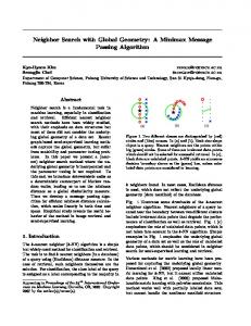
each time with hundred iterations inside the LDPC decoder. We did not iterate between the LDPC decoder and the mapper. The phase ambiguity was resolved by testing the M possible hypotheses. In the particle filtering algorithms, the messages were represented as lists of 100 samples; in the numerical integration algorithms, the phase was uniformly quantized over n = 100 levels. In the gradient methods, we optimized the (constant) step size parameter λ. In Figures 5 and 6, the phase synchronizers are compared in terms of mean squared (phase) estimation error (MSEE) and the decoded frame error rate (FER) as a function of the SNR respectively; the figures show that the particle filter algorithms have the best performance, followed by the algorithms based on numerical integration and then by the gradient methods—the more accurate the phase messages are represented, the better the performance. 0
10
Num. Integration (Constant Phase) Num. Integration (Random Walk, σ = 0.001) Num. Integration (Random Walk, σ = 0.01) Gradient Method (Constant Phase) Gradient Method (Random Walk, σ = 0.001) Gradient Method (Random Walk, σ = 0.01) Particle Filter (Constant Phase) Particle Filter (Random Walk, σ = 0.001) Particle Filter (Random Walk, σ = 0.01)
−1
−2
−3
−1
−0.5
0
0.5
1
1.5 E /N [dB] b
Fig. 5.
2
2.5
3
3.5
4
3
3.5
4
0
Mean squared estimation error.
0
10
−1
FER
10
−2
10
−3
10
Known phase Num. Integration (Constant Phase) Num. Integration (Random Walk, σ = 0.001) Num. Integration (Random Walk, σ = 0.01) Gradient Method (Constant Phase) Gradient Method (Random Walk, σ = 0.001) Gradient Method (Random Walk, σ = 0.01) Particle Filter (Constant Phase) Particle Filter (Random Walk, σ = 0.001) Particle Filter (Random Walk, σ = 0.01)
−4
10
−1
−0.5
0
0.5
1
1.5 E /N [dB] b
Fig. 6.
2
2.5
ACKNOWLEDGMENT This project was supported in part by the Swiss National Science Foundation grant 200021-101955. We heavily used the collection of C programs for LDPC codes by Radford M. Neal from R EFERENCES
10
10
V. C ONCLUSION We have presented several message passing algorithms, applicable to several channel models, for joint decoding and phase estimation. In contrast to prior and parallel work on such schemes by other authors, we have emphasized the systematic exploration of such algorithms starting from a factor graph of the channel model.
http://www.cs.toronto.edu/˜radford/ldpc.software.html.
MSEE
10
rithms based on numerical integration are much more complex. As is well known, numerical integration becomes infeasible in high-dimensional systems. The particle methods are complex as well, but they scale better with the dimensionality of the system.
0
Frame error rate.
The gradient methods have the lowest complexity, since the messages are represented by only a few parameters. The algo-
[1] D. Lee, “Analysis of Jitter in Phase-Locked Loops,” IEEE Trans. Circuits Syst. II, vol. 49, no. 11, Nov. 2002, pp. 704–711. [2] Q. Huang, “Phase Noise to Carrier Ratio in LC Oscillators” IEEE Trans. Circuits Syst. I, vol. 47, no. 7., Jul. 2000, pp. 965–980. [3] T. Lee and A. Hajimiri, “Oscillator Phase Noise: A Tutorial” IEEE J. Solid-State Circuits, vol. 35, no. 3., Mar. 2000, pp. 326–336. [4] A. Demir, A. Mehrotra and J. Roychowdhury, “Phase Noise in Oscillators: A Unifying Theory and Numerical Methods for Characterization” IEEE Trans. Circuits Syst. I, vol. 47, no. 5, May 2000, pp. 655–674. [5] A. Burr and L. Zhang, “Application of Turbo-Principle to Carrier Phase Recovery in Turbo Encoded Bit-Interleaved Coded Modulation System,” Proc. 3rd International Symposium on Turbo Codes and Related Topics, Brest, France, 1–5 Sept., 2003, pp. 87–90. [6] I. Sutskover, S. Shamai and J. Ziv, “A Novel Approach to Iterative Joint Decoding and Phase Estimation,” Proc. 3rd International Symposium on Turbo Codes and Related Topics, Brest, France, 1–5 Sept., 2003, pp. 83– 86. [7] H. Steendam, N. Noels, M. Moeneclaey, “Iterative Carrier Phase Synchronization for Low-Density Parity-Check Coded Systems”, International Conference on Communications 2003, Anchorage, Alaska, May 11–15, 2003, pp. 3120–3124. [8] N. Noels et al., “Turbo synchronization : an EM algorithm interpretation”, International Conference on Communications 2003, Anchorage, Alaska, May 11–15, 2003, pp. 2933–2937. [9] V. Lottici, M. Luise, “Carrier Phase Recovery for Turbo-Coded Linear Modulations”, International Conference on Communications 2002, New York, NJ, 28 April–2 May, 2002, vol. 3, pp. 1541–1545. [10] R. Nuriyev and A. Anastasopoulos, “Analysis of joint iterative decoding and phase estimation for the noncoherent AWGN channel, using density evolution,” Proc. 2002 IEEE Information Theory Workshop, Lausanne, Switzerland, June 30 – July 5, 2002, p. 168. [11] B. Mielczarek and A. Svensson, “Phase offset estimation using enhanced turbo decoders,” IEEE International Conference on Communications, ICC 2002, vol. 3, 28 April–2 May, 2002, pp. 1536–1540. [12] H. -A. Loeliger, “An introduction to factor graphs,” IEEE Signal Processing Magazine, Jan. 2004, pp. 28–41. [13] F. R. Kschischang, B. J. Frey, and H.-A. Loeliger, “Factor graphs and the sum-product algorithm,” IEEE Trans. Inform. Theory, vol. 47, pp. 498– 519, Feb. 2001. [14] H.-A. Loeliger, “Some Remarks on Factor Graphs”, Proc. 3rd International Symposium on Turbo Codes and Related Topics, 1–5 Sept., 2003, pp. 111–115. [15] M. Meyr, M. Moeneclaey and S. A. Fechtel, Digital Communication Receivers: Synchronization, Channel Estimation and Signal Processing, New York, John Wiley & Sons, 1998, pp. 246–249. [16] A. Doucet, N. de Freitas and N. J. Gordon, eds., Sequential Monte Carlo Methods in Practice, New York, Springer-Verlag, 2001.