Joint Motion and Color Statistical Video Processing for Motion

JOINT MOTION AND COLOR STATISTICAL VIDEO PROCESSING FOR MOTION SEGMENTATION Alexia Briassouli, Vasileios Mezaris, Ioannis Kompatsiaris Informatics and Telematics Institute Centre for Research and Technology Hellas ABSTRACT Vast amounts of digital multimedia data are being produced and distributed today, so methods for the efficient and reliable extraction of information from video data are becoming necessary. We present a novel motion segmentation algorithm, which accurately extracts moving objects from a video, and also provides a likelihood map, for each object pixel assignment. The flow is estimated, and accumulated over several frames, to give action masks. Color segmentation clusters regions of similar color in each frame. A novel, likelihood ratio-based method for the statistical comparison of color layers in the regions of activity and the background is presented and compared with an Earth Mover’s Distance-based approach. Our method also gives the likelihood with which each pixel is assigned to a moving object in each frame. Experiments with real sequences illustrate the advantages of our method, namely that it gives overall more reliable results, and also provides the likelihood map for the segmented object. 1. INTRODUCTION The facility with which digital multimedia can be acquired, created and disseminated today has increased the need for the efficient extraction of useful information from it. Computer vision and video processing tasks, such as the reliable segmentation of moving objects in video, have become more necessary than before. This paper focuses on the problem of segmenting moving objects from video, by integrating the motion and the color information in a statistically substantiated, and computationally inexpensive manner. Numerous methods have been proposed for the segmentation of moving objects [1], [2]. Object motion is a fundamental cue in these approaches, but using motion information alone may lead to inaccuracies, because of errors that may appear in the motion estimates. This motivates us to also employ the color information in the video [3]. Color segmentation alone does not suffice to extract moving objects from the video either, since a moving entity may be composed of many different colors. In this paper we present a novel method for integrating the motion information with the color segments, in order to achieve reliable motion segmentation. Sec. 2 presents the motion processing stage. The optical flow is estimated between pairs of frames, and then accumulated and processed statistically to form “action masks”, encompassing all pixels that have undergone a displacement. In the case of a moving camera, its motion can be compensated for in a pre-processing stage, and our method can be applied to the resulting video. Color segmentation is then applied to each frame, giving layers of color in the action masks and their complementary (background) regions (Sec. 3). Finally, two different approaches for matching the colors layers in the action masks and the background of each frames are described in

1-4244-1017-7/07/$25.00 ©2007 IEEE

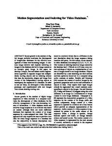
Sec. 4. Experiments demonstrate the effectiveness of our approach in Sec. 5, and conclusions and ideas for future work are shown in Sec. 6. 2. OPTICAL FLOW ANALYSIS FOR ACTION AREAS In order to localize the moving objects in the video sequence, we estimate the optical flow between pairs of frames, using the Lukas Kanade algorithm [4]. Since it is based on the constant illumination assumption, optical flow suffers from inaccuracies introduced by illumination changes that are not introduced by object motions (e.g. lighting changes, measurement noise). Although the Lukas Kanade method is more robust to these inaccuracies than other methods, the flow estimates are still noisy. Also, their values are higher near motion boundaries, and negligible in smooth areas of moving objects. In Fig. 1(a) and Fig. 4(a), the flow between pairs of video frames is significant only at the moving object boundaries. We take advantage of the velocity estimates’ noise, to extract action masks in each video sequence, with the pixels that undergo displacements during several (if not all) frames. Since we have many samples of this noise (it affects the flow estimates over all frame pixels, over many frames), we approximate it by a Gaussian distribution. Thus, finding moving pixels is reduced to testing if the accumulated velocity estimates follow a Gaussian distribution. For a random variable y, the classical measure of non-gaussianity is the estimation of its fourth order cumulant, also known as the kurtosis: kurt(y) = E{y 4 }−3(E{y 2 })2 . The fourth order moment of Gaussian random variables is given by E{y 4 } = 3(E{y 2 })2 , so ideally the kurtosis of a Gaussian random variable should be equal to zero. Motivated by this, we accumulate the flow estimates v for each pixel, over several frames, and characterize each pixel according to:  r¯ ∈ action area if E{v 4 } = 3(E{v 2 })2 (1) r¯ ∈ background if E{v 4 } = 3(E{v 2 })2 . The number of frames is chosen as follows: initially the mean of each pixel velocity is estimated over ten frames. We accumulate flow over new frames, and compare it with the mean of the previous frames. When a new estimate is greater than the standard deviation of the previous ones, we consider that an event has occurred, and therefore we have a sufficient number of frames. Naturally, it is possible to gather more frames, to include more than one event. We then estimate the kurtosis of each pixel’s flow estimates over the frames being examined. Since the Gaussian model is only an approximation, we do not expect the kurtosis to be zero, but we do expect it to be significantly higher at pixels that have undergone motion. We consider that pixels whose flow has kurtosis above 10% of the mean kurtosis have been displaced. These pixels form an “action maksk”, as in Fig. 1(b), where it is obvious that our method correctly localizes the moving pixels for a tennis match.

2014

ICME 2007

Optical flow between frames 9 and 10

4.1. Earth Mover’s Distance

Activity Mask for Tennis Match

(a)

There exist many methods for the comparison of the color in the action areas and the static frame pixels. For each color layer, we extract three histograms corresponding to its three color components. The histograms of each color can be regarded as “signatures” characterizing its distribution1 . A measure of the similarity between signatures of data is the Earth Mover’s Distance (EMD) [5], that calculates the cost of transforming one signature to another. A histogram with m bins, can be represented by P = {(μ1 , Σ1 , h1 ), ..., (μm , Σm , hm )}, where μi , Σi are the mean and covariance, respectively, of the data in that bin (equivalently, cluster), and hi is the corresponding histogram value (essentially the probability of the values of the pixels in that cluster). This histogram can be compared with another, Q = {(μ1 , Σ1 , h1 ), ..., (μn , Σn , hn )}, by estimating the cost of transforming histogram P to Q. If the distance between their clusters is dij (we use the Euclidean distance here), the goal of transforming one histogram to the other is that of finding the flow fij that achieves this, while minimizing the cost:

(b)

Fig. 1. (a) Optical flow between frames 9 − 10. (b) Activity mask.

3. COLOR-BASED FRAME SEGMENTATION The activity masks described in the previous section include any pixel that moves during a subsequence of the video, so color processing is used for the precise localization of the moving objects in each frame. We perform color segmentation with the mean shift algorithm [3], as it is reliable, and does not require determining the number of clusters. Mean shift searches for the modes of the data’s distribution, so their number “automatically” gives the number of clusters. This search is performed over a window of radius h, which we set equal to the percentage of each frame that is covered by the action mask. This makes intuitive sense and, indeed, leads to accurate results, since the size of the moving entities determine the size of the action mask. We approximate the data’s distribution by a distribution with a symmetric kernel K(x), as follows: fˆ(x) =

  n 1  x − xi K , nhd i=1 h

(2)

and then search iteratively for the distribution’s modes. The Epanechnikov kernel is used, as it is symmetric and differentiable, and thus enables us to calculate the distribution’s gradient and its modes.  KE (x) =

1 −1 c (d 2 d

+ 2)(1 − xT x), if xT x < 1 0, otherwise

(3)

The modes of the data distribution are reached by translating the data window by the “sample mean shift”: Mh (x) =

1  xi − x. nx x ∈S i

(4)

h

W =

n m  

dij fij .

(5)

i=1 j=1

Once the optimal flow fij is found [5], the EMD becomes: m n i=1 j=1 dij fij . EM D(P, Q) = m n i=1 j=1 fij

(6)

We estimated the EMD between the three histograms of each color layer in the action mask and the background area of each frame. We combined the EMD’s results for each color by simply adding their magnitudes. The color layers of the static areas and the action areas that require the least cost (EMD) to be transformed to each other should correspond to pixels with the same color. Indeed, our experiments show that this approach correctly separates the background pixels in the action areas from the moving objects. 4.2. Probability Likelihood Testing for Color Comparison In this section, we present an alternative approach to using the EMD, as it is computationally expensive, especially for large amounts of data and many color layers. This method has the advantage of providing an estimate of each pixel’s likelihood to belong to the moving object, in addition to leading to a binary decision, like the EMDbased comparison. We propose to estimate the statistical distribution of each layer’s colors in the action masks and the background areas, and compare them by likelihood ratio testing. This leads to a hypothesis test for each pixel r¯, with the hypotheses that it is “active” (i.e. has moved in the current frame) or “static” (i.e. it is a background pixel):

Once iterations converge to several density maxima, the image pixels are assigned to the clusters whose color is closest to their color.

H0 : r¯ ∼ fstatic (¯ r) H1 : r¯ ∼ factive (¯ r).

4. OBJECT SEGMENTATION FROM COLOR AND MOTION STATISTICAL ANALYSIS

This process requires modelling of the color data’s statistical distribution in both the action mask (factive ), and its complement (fstatic ). We make the realistic assumption that the three color components in each layer are independent random variables, so the overall pdf of each pixel r¯, in each layer, can be written as:

In order to isolate moving objects in each frame, we apply color segmentation to the pixels inside the action masks and to those outside these masks. The resulting color segmentation results need to be compared, in order to find which pixels of each frame’s action mask match the background color, and consequently which ones belong to a moving object in that frame.

flayer (¯ r) = fR (¯ r)fG (¯ r)fB (¯ r),

(7)

(8)

1 In [5] signatures have a more general meaning than histograms, but in this paper we consider the special case of histograms as signatures.

2015

where “layer” is static or active. Spatial luminance data is often modelled by mixtures of Gaussian distributions, which are estimated using the Expectation-Maximization (EM) algorithm [6]. However, the EM is computationally expensive, it requires knowing the number of mixture components, and its success is highly dependent on correct training, which limits its usability in general applications. For these reasons, we develop a simpler but effective method for approximating the color layer statistics, and subsequently comparing the different color regions. Fig. 2(a) shows the normal probability plot of the R component of a color layer inside an action mask, which shows that it follows a distribution with heavier tails than the Gaussian, as it contains outliers. We account for the data’s outliers by using the heavy-tailed Cauchy distribution, given by: f (x) =

1 γ , π γ 2 + (x − δ)2

(9)

where γ is the data’s dispersion and δ is its location parameter (the median for the Cauchy pdf). The dispersion expresses the data’s spread around δ, so it is equivalent to the data variance [7]. Normal Probability Plot for R color component in action area

Likelihood ratio values for the first color layer

0.999 0.997 0.99 0.98

the flexibility to decide whether the segmentation should include all possible object pixels, at the cost of including “false alarm” pixels, i.e. pixels that did not move at that frame, or including only the high LRT pixels, at the cost of losing some of the object pixels. 5. EXPERIMENTS In this section we show experimental results for real videos that demonstrate the effectiveness of our approach. Tennis Match: In these experiments we examine a video of a tennis match (Fig. 3(c)). Fig. 1 shows the motion analysis results, where the action areas are evident, and even the trajectory of the tennis ball has been extracted. It should be emphasized that this video was of particularly bad quality, yet the de-noising of the flow estimates successfully localized the active pixels. In Fig. 3(a), (b) we show the results of the color segmentation, where we can already discern the players from the tennis court. In this experiment, the color comparison using the EMD and the LRT gave the same segmentation result, shown in Fig. 3(d). Note that, in this sequence, the player in the back was not moving significantly, and was barely visible due to the poor quality of the sequence, so she has not been recovered.

Probability

0.95 0.90

Color segmentation for background

0.75

Color segmentation in action mask

0.50 0.25 0.10 0.05 0.02 0.01 0.003 0.001

50

100

150

200

Data

(a)

(b)

Fig. 2. (a) Normal Probability Plot of the red color component in an action mask’s color layer. (b) LRT for the same color layer. A likelihood ratio test (LRT) is then formulated, to find whether each frame’s pixel belongs to the color layer of the action or the static area. Using the Cauchy model for our data and Eq. (8), we have: 2 factive (¯ r) + (x − δactive )2 γstatic γactive , (10) = 2 fstatic (¯ r) γactive γstatic + (x − δstatic )2   i i where γlayer = i={R,G,B} γlayer , δlayer = i={R,G,B} δlayer (layer = static or active) are estimated directly from the data available [7]. In order to mask out the player, we threshold the values of the LRT, using the Bayesian threshold [8], which is automatically extracted from the data:

(a)

(b)

Frame 47 for tennis match

Segmentation result for tennis match

(c)

(d)

L(¯ r) =

η=

μH1 + μH0 , 2

(11)

where μH1 and μH0 are the means of the LRT. They are directly estimated from the data available as follows: μH1 = EH1 [L(¯ r)], μH0 = EH0 [L(¯ r)], where, for H1 we estimate the LRT mean using factive , and for H0 we use fstatic . By thresholding the LRT, we separate the moving object pixels from the background pixels in each frame. As our experiments show, this method gives equally good results as the EMD-based one, and in some cases performs even better, at a much lower computational cost and with a simpler implementation. Another advantage of using the LRT is that it gives the likelihood with which the pixels in the action mask match the corresponding color layer of the static regions, as shown in Fig. 2(b). This gives us

Fig. 3. Frame 47 of Tennis match. Color segmentation for (a) background areas, (b) action masks. (c) Frame 47. (d) Final segmentation. Tennis Serve: Experiments were also conducted with a video showing a player serving a tennis ball (Fig. 5(a)). Fig. 4 shows characteristic flow estimates, and the resulting action mask. The results of the mean-shift color segmentation are shown in Fig. 4(c), (d) where we see that the player’s colors help separate her from the background. The final segmentation results using the EMD and LRT are shown in Fig. 5(b) and (c) respectively. In this case, the LRT gave better segmentation results than the EMD. This can be attributed

2016

Optical flow between frames 19 and 20

Activity Area for frames 1 to 60

Frame 4 for tennis serve

(b)

(a)

(a) Color segmentation in the action mask

Color segmentation for background area

(c)

Segmentation result using the EMD

(b) Segmentation result using the LRT

(d)

(c)

Fig. 4. Tennis serve. (a) Optical flow between frames 19 and 20. (b) Action mask. Color segmentation: (c) action mask, (d) background.

Fig. 5. (a) Frame 4 of Tennis serve. (b) EMD-based segmentation. (c) LRT-based segmentation.

to the fact that the test based on the EMD sums the absolute values of the EMD’s between the three color components, whereas the LRT makes the more realistic assumption that the color distributions are independent, and approximates the total pdf by multiplying the marginal pdfs (Eq. 8). In our experiments with the rest of the video frames, we found that, overall, the EMD and LRT based approaches perform comparably, with the LRT method giving better results in some cases (like that of Fig. 5). Also, the computational cost of the EMD method is higher, as it involves an optimization process for comparing all possible combinations of the color histogram bins. In the experiments, on a 3.4 GHz Pentium IV, using Matlab, the EMD algorithm takes 0.095 seconds per 720 × 576 frame, and the LRT estimation 0.024 seconds.

7. REFERENCES [1] G. D. Borshukov, G. Bozdagi, Y. Altunbasak, and A. M. Tekalp, “Motion segmentation by multistage affine classification,” IEEE Transactions on Image Processing, vol. 6, no. 11, pp. 1591– 1594, Nov. 1997. [2] J. Mansouri, A.-R.; Konrad, “Multiple motion segmentation with level sets,” IEEE Transactions on Image Processing, vol. 12, no. 2, pp. 201–220, Feb. 2003. [3] Comaniciu V. and Meer P., “Mean shift: A robust approach toward feature space analysis,” IEEE Transactions on Pattern Analysis and Machine Intelligence, vol. 42, no. 5, pp. 603 – 619, May 2002. [4] Kanade T. Lukas B., “An iterative image registration technique with an application to stereo vision,” in International Joint Conference on Artificial Intelligence, 1981, pp. 674–679.

6. CONCLUSIONS This paper proposes a novel method for the accurate segmentation of moving objects in a video, that is computationally efficient, and produces a likelihood map for the segmentation. Optical flow estimates are processed statistically to give action masks, with the pixels that move during the video. These masks are integrated with color segmentation by comparing the color layers via the EMD and a novel LRT-based method. The latter has the novel feature of giving likelihood estimates for each pixel in the action mask, so that a pixel can be assigned to a moving object with high or low probability in each frame. Experiments demonstrate the accuracy of the object segmentation and the usefulness of the likelihood maps. Acknowledgments: This work was supported by the European Commission under contracts FP6-001765 aceMedia, FP6-027685 MESH and FP6-027026 K-Space and by the GSRT funded project DELTIO: Analysis of Multimedia Content using Evolutionary Ontologies and Application to Television News Bulletins.

[5] Rubner Y., Tomasi C., and Guibas L. J., “The earth movers distance as a metric for image retrieval,” International Journal of Computer Vision, vol. 40, no. 2, pp. 99 – 121, 2000. [6] Priebe C. E. and Marchette D. J., “Adaptive mixture density estimation,” Pattern Recognition, vol. 26, no. 5, pp. 771–785, 1993. [7] Hanson K. and Wolf D., “Estimators for the cauchy distribution,” in Maximum Entropy and Bayesian Methods in Science and Engineering, G. Heidbreder, Ed., pp. 255–263. Kluwer Academic, Dordrecht, 1996. [8] H. V. Poor, An Introduction to Signal Detection and Estimation, Springer-Verlag, New York, second edition, 1994.

2017