Motion Segmentation and Indexing for Video ... - INTELLIGENCE

Motion Segmentation and Indexing for Video Database.∗ King Yuen Wong Minas E. Spetsakis Department of Computer Science York University Toronto, Ontario Euripides G. M. Petrakis† Dept. of Electronic and Computer Engineering Technical University of Crete E-mail: [email protected], [email protected], [email protected]

ABSTRACT Recent growth in the number of digital images available motivates the development of image/video databases for the effective management of these ever-increasing images. A common image retrieval task requires retrieving all images in the database similar in image content to an example query image. In this paper, we develop a simple, fast and robust motion segmentation algorithm to separate images into independently moving objects and an indexing scheme that uses the trajectories, shapes and image flow vectors of the independently moving objects to insert/query the sequences in a database. In order to test our ideas, we developed a video database prototype and experimented with real images from scenes showing moving cars.

result in a retrieval failure due to a difference in the text description about the image sequence during insertion and query. For this reason, recent research in video databases (for example [5, 6, 9, 14, 21, 24, 22]) focuses on indexing based on image content by the database itself. Niblack et al [21] use color, texture and shape of objects as a representation of content of images stored in an image database. Objects are identified by a user sketching out their outlines and then optimally traced out in a computer using active contours or snakes. Petrakis and Faloutsos [24] measure the content of medical images by the geometric properties such as size and orientation of objects in them. They require their input images already be segmented into closed contours corresponding to objects in the images. Das and Riseman [5], Huang and Kumar [14] suggest using the color 1. Introduction attributes in an image as a measurement of image Recent growth in the number of digital image content in color image databases. Hampapur et al sequences or video available in a computer moti- [9] represent the characteristic properties of a video vates the development of video databases for the sequence by the content of its image, audio and effective management of the ever-increasing vol- motion components. Image content of a video ume of information. A video database stores and sequence is captured in a minimal set of key frames retrieves image sequences in an efficient way based which provide an adequate representation of the on content although there are more traditional sequence. Audio content of a video sequence is repdatabases that represent the content of an image resented by points in the audio stream of the sequence by a user-assigned text label. This later sequence where a change in speaker, change approach not only requires the user to provide a text between speech and music, or change between label for every image sequence in a database but silence and sound occurs. The motion content of a also the subjectivity in human descriptions may video sequence is represented by the total amount of motion, uniformity of motion in the sequence ∗The support of the NSERC (App. No. OGP0046645) is gratefully acknowledged. †Part of the work was carried out while the third author was visiting York U.

Moving Image Database

etc. Deng et al [6] represent the content of a video sequence by the color, texture, shape, size, location and motion of sub-objects in the sequence. Subobjects are segments identified by their spatio-temporal segmentation algorithm which works by first identifying color/texture coherent blobs and then fitting an affine image flow motion model to each of these blobs. A video can be broken into “shots” (i.e., meaningfull units of video information corresponding to frame sequences between two stop camera operations or frame sequences with similar motion characteristics). A “scene” is a collection of shots characterized by a common event. A “clip” consists of one or more scenes. The clip/scene/shot structure defines a hierarchy of video information [29] A shot can be considered as the foundamental retrievable video entity. Video retrieval can be based on features computed to shots. Various approaches to shot detection have been proposed. Most of them as reviewed in [18, 4]. Before a video is stored, it has to be segmented into shots and appropriate features are computed to the extracted shots. These features can then be used for video retrieval [29] Video content in each shot is given in terms of features of contained objects and of their motion. Unlike approaches performing on compressed MPEG video [17, 23]our video segmentation algorithm works on uncompressed video by detecting spatio-temporal changes in subsequent frames. In addition, we deal with multiple objects and with their interelationships. In this paper, we present an approach to moving image databases that uses motion segmentation and an indexing scheme based on shape and trajectory. We developed a moving image database prototype for sequences showing objects undergoing piecewise constant motion, e.g. image sequences showing car racing and horse racing. Moving objects in the dynamic scene are identified by our motion segmentation algorithm. Pixels belonging to the same independently moving object move with similar velocities and hence share similar image flow [11]. By analyzing the structure of image flow, aggregating pixels having similar flows into blobs and tracking of these blobs over frames in the sequence, we have a means of identifying independently moving objects in the dynamic scene. In other words, our image flow coherence model is piecewise constant flow within each frame and maximal overlap across successive frames. We represent the image content

Wong, Spetsakis, Petrakis

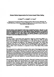
of an image sequence by calculating some statistics, such as shapes, trajectories, image flows of these spatio-temporal coherent blobs and use these as components of the feature vector representing the dynamic scene in the image sequence. Then we store the image sequence into our moving image database using its feature vector as an index. Finally, we support content-based image sequence retrieval by first computing the feature vector associated with the query image sequence and use that as an index to the moving image database to retrieve all image sequences that undergo similar motion as the query sequence. Using different statistics, we can modify the meaning of similarity. 2. Motion segmentation algorithm We develop a simple, fast and robust motion segmentation algorithm for images under piecewise constant motion. Our algorithm works by first identifying strong edges, classifying them based on image flow and then propagating the classified labels to non-edge pixels. In essence, we are propagating image flow from regions where flow estimation is reliable to regions where flow estimation is ill-conditioned. Furthermore, by first classifying strong edges, our algorithm produces clear and highly localized motion boundaries because we only propagate image flow values within the boundary of an object. Moreover, the underlying concept is simple and intuitive as our algorithm is only based on strong edge classification and smooth variation of flow values within the surface of the objects. As a result, our algorithm runs quite quickly. In the following, we outline the steps involved in our algorithm for the image frame pair in Fig 2.1.

Fig 2.1 continued...



through every pixel in the frame pair , we find N peaks in the Hough space (that is (u1 , v 1 ), .. , (u N , v N )) by iteratively detecting a global maximum and then removing votes that correspond to the maximum just found [25]. Phase 2: Aggregating neighboring pixels having similar flow into regions following a bottom-up paradigm. Fig 2.1. There are three major phases involved in our motion segmentation algorithm. Phase 1: Identification of image flow vectors for the independently moving objects by Hough Transform We identify N image flow vectors {(u1 , v 1 ) , .. , (u N , v N )} using Hough Transform. Borrowing idea from Lucas and Kanade [20], we smooth image flow constraints at a pixel with a Gaussian filter over a small neighborhood so that the image flow equation (I x u + I y v + I t = 0 [12]) is applicable to a small neighborhood of the image frames in the least squares sense.  E xx   E yx

E xy  u −E xt  = ⋅  E yy   v  −E yt 

We detect strong edges (which correspond to boundaries of objects in the dynamic scene [28]) by a combination of methods including Canny edge detection [2], heuristic edge contour tracing across a pyramid of images which are produced by smoothing an image with Gaussian filters of various scales (σ s) [1, 3, 19] and joining of contour end points [7]. Afterwards, we classify the edges by assigning a label to each edge pixel that best satisfies the flow constraint [16]. In particular, for every edge pixel, we assign to it a class label m (which corresponds to flow vector (u m , v m )) that minimizes the following: min ||I x ui + I y v i + I t ||

1≤i≤N

(2.3)

(2.1)

where E xx = (I x2 )(*)g the result of the convolution of the square of the image derivative with a gaussian and E xy etc are respectively the results of similar convolutions. This can be shown to be the region matching constraint where the region is defined by the gaussian window and it generates a more accurate flow field estimation Hence, flow field (u, ˆ v) ˆ can be calculated using the pseudo-inverse matrix as follows:

We go through the image first in a direction orthogonal to the dominant flow vector direction 1 and then in the direction of dominant flow vector. 0   V 0x V 0y  −E xt  uˆ   V 0x V 1x   A dominant flow vector is the nonzero vector that  λ 0  = ⋅  ⋅ (2.2)   1 ⋅ V 1x V 1y  −E yt  has the biggest norm in the set of flow vectors in   vˆ   V 0y V 1y   0 λ1  phase one. At each row/column, we assign to every Each estimated image flow (u, ˆ v) ˆ is inside a cloud unclassified pixel between a pair of successive edge of uncertainty in the shape of an ellipse [26]. The pixels that have been assigned to the same class probability of (u, ˆ v) ˆ is scattered along principal axes label c if all classified pixels in between these edge of the elliptical cloud in a way proportional to pixels have also been assigned the label c. reciprocals of the square root of eigenvalues of the covariance matrix. The principal axes of the ellipse cloud lie along eigenvectors of the covariance E E xy  matrix  xx . At each pixel, we vote into the  E yx E yy  Hough space by plotting a straight line centered at (u, ˆ v) ˆ with length and direction that of the major axis of the cloud of uncertainty. After going


We identify the unclassified connected regions using a sequential labeling algorithm [11]. For each unclassified connected region surrounded by a boundary in which the majority of labels is assigned the class c, we assign the label c to the region.

Borrowing ideas from Susan and Jain [10], we perform moving edge detection by running Canny edge detection on temporal image derivative I t . Afterwards, we perform motion based classification of those temporal edge pixels which have not been classified.

We identify the remaining unclassified connected regions using the sequential labeling algorithm. For each unclassified connected region, we assign to every pixel in the region a label that minimizes the weighted sum of flow constraint equations of all pixels inside the connected region.


Phase 3: Post-processing steps for reducing effects caused by noise. In this phase, we perform size and morphological filtering [15] on the segmented image. These are post processing steps for alleviating the effects caused by noise and phenomena such as shadows, specular reflections and uneven illumination that violate the data conservation model in motion. After performing size filtering on the segmented image, it becomes:

After performing morphological filtering on the segmented image, it becomes:

Finally, we create a flow field corresponding to the segmented image.



pcampolr1.pgm to pcampolr4.pgm, which shows a

police car chasing a sports car (Fig. 4.1). Using shapes, trajectories and image flow of objects as a measurement of similarity, our database outputs:

3. Statistics used in feature vector for image sequence Statistics that we used for representation of image content are:

MM>queryVDB(3,["pcampolr1.pgm","pcampolr2.pgm", "pcampolr3.pgm","pcampolr4.pgm"],:closestK=15, :saveDist="shape2.dat"); [["pcampol7.pgm","pcampol8.pgm","pcampol9.pgm", "pcampol10.pgm"], ... ["camtru2.pgm","camtru3.pgm","camtru4.pgm", "camtru5.pgm"], ... ["campol2.pgm","campol3.pgm","campol4.pgm", "campol5.pgm"], ...

1) Shapes of the independently moving objects. These are represented by some moment measures of the regions in the segmented images which are invariant to translation, rotation and scaling [13].

The most similar sequence is pcampol7.pgm, .., pcampol10.pgm. The distance between the feature

2) Trajectories of the independently moving objects. These are represented by the center of gravity of the segmented regions over frames in the video sequence.

The second most similar sequence is camtru2.pgm, .., camtru5.pgm (ignoring siblings of pcampol*.pgm, sibling sequences are subsequences that are derived from the same sequences), which is the 8th closest sequence. The distance between the feature vector of the query sequence and that of this sequence is 172.205 (Fig. 4.3).

3) Image flow of the independently moving objects. (Image flow velocities are proportional to velocities of objects in a dynamic scene.) 4) Orientations of the image flow vectors. We store the angle between the line joining any two moving regions and their relative velocities. 5) Normalized sizes of the independently moving objects. 6) Time to collision measures amongst independently moving objects. It is defined by atan2(d, v) where d is the distance between the center of gravities of the two objects/regions and v is their relative velocity projected on the line joining the center of gravities of the two objects/regions. If there are more than 2 moving objects, we store a time to collision measure for every possible pair of moving objects. 4. Experiments In this section, we present the result of a typical query in our moving image database prototype. The moving image database prototype is implemented using MediaMath [27]. In order to increase the number of items in the database, we divide every sequence into shorter subsequences and insert/query each subsequence separately. For the query using the video sequence

vector of the query sequence and that of this sequence is 60.272 (Fig. 4.2).

In the following figure, we plot the Euclidean distance between the feature vector of the query sequence and those of the 15 most similar sequences sorted in ascending order of dissimilarity. Note the existence of subsequences that are derived from the same input sequence. Distance 200 180 160 140 120 100 80 60 0

’shape2.dat’

2 4 6 8 10 12 14 16 Best 15 sequences similar to the query

Euclidean distance between the feature vector of the query and 15 most similar sequences This graph presents the 15 sequences similar to the query sorted in ascending order of distance to the



query. We see a sharp transition from siblings sequences to similar but non sibling sequences.

sizes, shapes and image flow of the segmented objects. We assume piecewise constant motion.

Using sizes of the moving objects as a measurement of similarity with the same query pcampolr*.pgm as before, our database outputs:

In future research, we will experiment affine motion models, flow prediction and the use of efficient database organization schemes like multidimensional R-trees [8].

MM>queryVDB(3,["pcampolr1.pgm","pcampolr2.pgm", "pcampolr3.pgm", "pcampolr4.pgm"], :trajectoryFlag=nil,:shapeFlag=nil,:velocityFlag=nil,:sizeFlag=t, :closestK=15,:saveDist="size2.dat"); [["pcampol3.pgm","pcampol4.pgm","pcampol5.pgm", "pcampol6.pgm"], ... ["campol4.pgm","campol5.pgm","campol6.pgm","campol7.pgm"], ... ["rcampol5.pgm","rcampol6.pgm","rcampol7.pgm", "rcampol8.pgm"]]

The most similar sequence is pcampol3.pgm, .., pcampol6.pgm. The distance between the feature vector of the query sequence and that of of this sequence is 0.0262 (Fig. 4.4). The next most similar sequence is campol4.pgm, .., campol7.pgm (ignoring the sequences that are siblings of pcampol*.pgm), which is the 8th closest

References 1.

F. Bergholm, “Edge Focusing,” IEEE Transactions on Pattern Analysis and Machine Intelligence 9(6) pp. 726-741 (1987).

2.

J. Canny, “A Computational Approach to Edge Detection,” IEEE Transactions on Pattern Analysis and Machine Intelligence 8(6) pp. 679-698 (1986).

3.

B. Chen and P. Siy, “Forward/Backward Contour Tracing with Feedback,” IEEE Transactions on Pattern Analysis and Machine Intelligence 9(3) pp. 438-446 (1987).

4.

A. Dailianas, R. Allen, and P. England, “Comparision of automatic video segmentation algorithms,” pp. 2-16 in Proceedings SPIE, Photonics East 1995Integration issues in large Commercial media delivery systems, , Philadelphia (1995).

5.

M. Das, E. M. Riseman, and B. A. Draper, “FOCUS: Searching for Multi-colored Objects in a Diverse Image Database,” pp. 756-761 in Proceedings / IEEE Computer Society Conference on Computer Vision and Pattern Recognition, (1997).

6.

Y. Deng, D. Mukherjee, and B. S. Manjunath, “NeTra-V: Towards an Object-based Video Representation,” pp. 202-213 in Proceedings of SPIE: Storage and Retrieval for Image and Video Databases VI, (1998).

7.

J. Eklundh, T. Elfving, and S. Nyberg, “Edge Detection using the Marr-Hildreth Operator with Different Sizes,” pp. 1109-1112 in Proceedings, 6th International Conference on Pattern Recognition: Munich Germany Oct 19-22, 1982, (1982).

8.

A. Guttman, “R-trees: a dynamic index structures for spatial searching,” pp. 47-57 in Proceedings ACM SIGMOD, (1984).

9.

A. Hampapur, A. Gupta, B. Horowitz, C. Shu, C. Fuller, J. Bach, M. Gorkani, and R. Jain, “Virage Video Engine,” pp. 188-197 in Proceedings SPIE: Storage and Retrieval for

sequence. The distance between the feature vector of the query sequence and that of this sequence is 0.0351 (Fig. 4.5). In the following, we plot the Euclidean distance between the feature vector of the query sequence and those of the 15 most similar sequences sorted in ascending order of dissimilarity. Note the existence of subsequences that are derived from the same input sequence. Distance 0.046 0.044 0.042 0.04 0.038 0.036 0.034 0.032 0.03 0.028 0.026 0

’size2.dat’

2 4 6 8 10 12 14 16 Best 15 sequences similar to the query Euclidean distance between the feature vector of thequery and 15 most similar sequences.

5. Conclusion We presented an approach to video databases that supports query by example that is based on motion segmentation and indexing based on trajectories,


Image and Video Databases V, (1997). 10.

S. M. Haynes and R. Jain, “Detection of Moving Edges,” Computer Vision, Graphics and Image Processing 21 pp. 345-367 (1983).

11.

B. K. P. Horn, Robot Vision, McGraw-Hill Book Company, New York (1986).

12.

B. K. P. Horn and B. G. Schunck, “Determining Optical Flow,” Artificial Intelligence 17 pp. 185-204 (1981).

13.

M. Hu, “Visual Pattern Recognition by Moment Invariants,” IRE Transactions on Information Theory 8 pp. 179-187 (1962).

14.

J. Huang, S. R. Kumar, M. Mitra, W. Zhu, and R. Zabih, “Image Indexing Using Color Correlograms,” pp. 762-768 in Proceedings / IEEE Computer Society Conference on Computer Vision and Pattern Recognition, (1997).

15.

R. Jain, R. Kasturi, and B. G. Schunck, Machine Vision, McGraw-Hill Inc. (1995).

16.

A. Jepson and M. J. Black, “Mixture Models for Optical Flow Computation,” pp. 760-761 in Proceedings / IEEE Computer Society Conference on Computer Vision and Pattern Recognition, (1993).

17.

V. Kobla, D. Dobermann, and C. Faloutsos, “Video Trails: Representing and Visualizing Structure in Video Sequences,” in Proceeding of ACM Multimedia 97, , Seattle (1997).

18.

R. Lienhart, S. Pfeiffer, and W. Effelsberg, “Video Abstracting,” Communications of the ACM 40(12) pp. 55-62 (1997).

19.

H. K. Liu, “Two and Three-Dimensional Boundary Detection,” Computer Graphics and Image Processing 6 pp. 123-134 (1977).

20.

B. D. Lucas, Generalized Image Matching by Method of Differences, Department of Computer Science, Carnegie-Mellon University (1984).

21.

W. Niblack, R. Barber, W. Equitz, M. Flickner, E. Glasman, D. Petkovic, P. Yanker, C. Faloutsos, and G. Taubin, “The QBIC Project: Querying Images By Content Using Color, Texture, and Shape,” pp. 173-181 in Proceedings of SPIE - The International Society for Optical Engineering: Storage and Retrieval for Image and Video Databases, (1993).


22.

J. M. Odobez and P. Bouthemy, Separation of Moving Regions from Background in an Image Sequence Acquired with a Mobile Camera, Kluwer Academic Publisher (1997).

23.

V N. Patel and I. K. Setchi, “Video Shot Detection and Charactrization for Video Databases,” Pattern Recognition, 30(4) pp. 583-592 (1997).

24.

E. G. M. Petrakis and C. Faloutsos, “Similarity Searching in Medical Image DataBases,” IEEE Transactions on Knowledge and Data Engineering 9(3) pp. 435-447 (1997).

25.

T. Risse, “Hough Transform for Line Recognition: Complexity of Evidence Accumulation and Cluster Detection,” Computer Vision, Graphics And Image Processing 46 pp. 327-345 (1989).

26.

A. Singh, “An Estimation-Theoretic: Framework for Image-Flow Computation,” pp. 168-177 in Proceedings, Third International Conference on Computer Vision, (1990).

27.

M. E. Spetsakis, “MediaMath: A research environment for vision research,” pp. 118-126 in Vision Interface, , Banf, Alberta (1994).

28.

W. B. Thompson, “Combining Motion and Contrast for Segmentation,” IEEE Transactions on Pattern Analysis and Machine Intelligence 2(6) pp. 543-549 (1980).

29.

B. L. Yeo and M. M. Yeung,, “Retrieving and Visualizing Video,” Communications of the ACM 40(12) pp. 43-52 (1997).



Fig. 4.1 Query sequence: pcampolr1.pgm to pcampolr4.pgm

Fig. 4.2: Most similar retrieved sequence: pcampol7.pgm, .., pcampol10.pgm (Shape-Trajectory)

Fig. 4.3: Second most similar retrieved sequence: camtru2.pgm, .., camtru5.pgm (Shape-Trajectory)

Fig. 4.4: Most similar retrieved sequence: pcampol3.pgm, .., pcampol6.pgm (Sizes)

Fig. 4.5: Second most similar retrieved sequence: campol4.pgm, .., campol7.pgm (Sizes)