Joint Rate Control and Routing for Energy-Constrained Wireless ...

Joint Rate Control and Routing for Energy-constrained Wireless Sensor Networks with the Real-time Requirement Meng Zheng, Wei Liang, Xiaoling Zhang, Haibin Yu, and Peng Zeng Abstract— In the following paper, we study the tradeoff between network lifetime and network utility for energyconstrained wireless sensor networks(WSNs) with the real-time requirement. By introducing a parameter r, we combine these two objectives into a single weighted objective, and consider rate control and routing in this tradeoff framework simultaneously. For real-time requirement, we set up real-time constraints by forcing the end-to-end delay of each route to be bounded by the maximum tolerated delay and incorporate real-time constraints into the tradeoff framework. Consequently, the tradeoff model is formulated nonlinear programming. By using the dual decomposition method and gradient/subgradient algorithms, we propose a distributed algorithm to solve nonlinear programming. Rigorous analysis and simulation are presented in order to validate our algorithm.

I. I NTRODUCTION Wireless sensor networks have become a key technology for the 21st century due to their widespread application in disaster alerts, structural health monitoring, industrial and factory automation, as well as many other applications. In WSNs, one important issue is energy constraint— wireless nodes usually carry limited and irreplaceable power supply[1]. Besides the energy constraint, real-time constraint is another concern in industrial applications, especially for industry wireless networks[2]. Thus in this paper we will concentrate on an energy-aware algorithm for energyconstrained WSNs with the real-time requirement. Since the seminal papers[3]-[4] were published, the network utility maximization (NUM) framework has been widely used to design congestion protocols. After that, multipath routing problem for wired networks[5]-[6] and wireless networks[7] was incorporated into this framework. Recently, energy-aware routing protocols for wireless sensor networks has been designed to maximize the network lifetime[8]-[11]. In these works, network lifetime was defined as the period from the time instant when the network starts functioning to the time instant when the first node runs out of energy[9]. The objective is to maximize the network lifetime while guaranteeing the required traffic rate. However, since sensor nodes are assumed to have fixed source rates, the network likely cannot sustain these rates for the given system resource This work was supported by the Natural Science Foundation of China under contact (60704046, 60725312, 60804067), the National 863 high technology research and development plan under contact (2007AA04Z173). Meng Zheng, Wei Liang, Xiaoling Zhang, Haibin Yu, and Peng Zeng are with Key Laboratory of Industrial Informatics Computer Engineering, Shenyang Institute of Automation, Chinese Academy of Sciences, Shenyang, 110016 China. Email: {zhengmeng 6, weiliang, zhangxiaoling, yhb,and zp}@sia.cn Meng Zheng and Xiaoling Zhang are with Graduate School of the Chinese Academy of Sciences, Beijing, 100039 China

constraint. Hence, a rigorous framework was proposed to study the network utility-lifetime tradeoff problem for the first time[12]. However, the subgradient based approach did not allow a fully distributed solution. Before long, Nama et al. improved upon their earlier results by proposing a fully distributed implementation[13]. For congestion control and routing coupled subproblem, Nama et al. appended the objective with a concave regulation term involving the flow variables and introduced some lifetime variables. As a result, the coupled subproblem was vertically decomposed into a congestion control problem and a routing problem. However, this transformation is only the approximation of the original problem. In addition, extra introduced lifetime variables bring too much communication overhead. Different from [12] and [13], Zhu et al. used the variable substitution method to transform the original problem into a single variable constrained optimization problem[14]-[15]. Thus their algorithms are derived based on an equivalent transformation. Additionally, extra lifetime variables are not needed. Besides the above mathematical decomposition technique, another remarkable approach to distributed solutions is to use game theoretic solutions[16]. Our study belongs to the series of [12]-[15]. However, in the above literatures[8]-[15], constraints on the rates of data transmission were mainly dictated by flow conservation laws, maximum link capacities, and energy conservation laws. No particular attention was paid to the real-time task performed by the WSN. As far as we know, the distributed algorithm for applications that require realtime delivery of data is still missing. In this paper, the delay on each link is expressed as a convex and increasing function with respect to the link rate. We set up real-time constraints by forcing the end-to-end delay of each route to be bounded by the maximum tolerated delay. Considering rate control and routing jointly, we formulate the network lifetime-utility tradeoff problem as a nonlinear programming. By dual decomposition method and subgradient algorithm, we derive a distributed algorithm that converges to the optimal scheme solving the nonlinear programming. Our work is similar to [14]-[15]. However, there are at least four differences. First, we remove the assumption that the network is under-loaded. Second, we consider the sensing energy that usually takes a non-negligible energy consumption in energy dissipation model. Third, our distributed algorithm can guarantee real-time requirement. Fourth, we describe the system model in the node-centric formulation method contrast to the link-centric formulation method[14][15]. The former three differences enable our algorithm to

978-1-4244-4148-8/09/$25.00 ©2009 This full text paper was peer reviewed at the direction of IEEE Communications Society subject matter experts for publication in the IEEE "GLOBECOM" 2009 proceedings.

be suited to wider application scenarios. The last difference makes our algorithm more robust than those of [14]-[15]. The rest of the paper is organized as follows. In Section II and Section III, we set up the network model. In Section IV, a distributed algorithm is developed for the network model. Section V presents numerical results and Section VI concludes this paper. II. NETWORK OBJECTIVE We consider a WSN that consists of a set V of sensor nodes that are indexed from 1 to N and a single sink that collects data from these nodes. There are two main metrics on the performance of WSNs, the network lifetime and the accuracy of information received at the sink node. In the following, we will define the two metrics in a rigorous mathematical formulation. A. Network Lifetime In a WSN, each sensor node is usually battery driven, non-rechargeable and irreplaceable. Thus, sensor nodes have much tighter energy constraints than the sink node. Here, we focus on the energy dissipated in the sensor nodes in this paper. Let Tv denote the lifetime of node v, v=1,2,· · ·,N, i.e., the time at which it runs out of energy. Definition 1[10]. We consider a general definition of network lifetime given by a concave function of the node lifetimes. In particular, we define Tnet = f (T1 , · · · , TN )

where sv is the rate allocation for source v and ωv is the weight associated with Uv (sv ). In this way, we can achieve weighted fairness on source rates of sensor nodes. C. Tradeoff between Network Lifetime and Network Utility There is an intrinsic tradeoff between network lifetime and network utility. By introducing a system parameter r ∈ [0, +∞), we can combine these two objectives together as a single weighted objective. The weighted objective function can be obtained as follows  rωv Uv (sv ) + Tnet (3) v∈V

Obviously, (3) degenerates to (1) for r = 0 and (2) for r → +∞. III. C ONSTRAINTS F ORMULATION We represent the WSN as a directed graph G(V, L), where L denotes the set of logical links. Let Lout (v) denote the set of outgoing links from node v, Lin (v) the set of incoming links to node v. Let R denote the set of routes. Each route r is assumed to carry data from a unique sensor to the sink. A. Flow Conservation Constraint On each link l, let fl denote the average amount of flow destined to the sink, cl the capacity of link l. Obviously, 0 ≤ fl ≤ cl

N

where f : R → R is a concave function in the vector of node lifetimes. In this paper, we just concentrate on the special case of Tnet = min(Tv ) v∈V

(1)

The lifetime maximization problem maximizes the time at which the first node dies, i.e., it minimizes the maximum ratio of average power consumption to initial energy among all nodes. Thus, the definition (1) balances the data flow in the network such that no node incurs a very high power consumption. B. Network Utility We use the utility function to describe the level of satisfaction attained by a source node. Different shapes of utility functions lead to different types of fairness. For example, the following family of utility functions, parameterized by α ≥ 0, is proposed in [18]:  (1 − α)−1 x1−α if α = 1 U α (x) = log x, otherwise When α = 1, the utility function guarantees to achieve proportional fairness; when α = 2, then harmonic mean fairness; when α → ∞, then max-min fairness. Based on the chosen utility function, we will adopt the NUM framework to study the rate allocation for WSNs. The objective function of the NUM can be formulated as  ωv Uv (sv ) (2) v∈V

(4)

For the sink, we define a source-sink vector s ∈ RN , whose vth entry sv denotes the source rate at node v. Therefore, we obtain the flow conservation constraint   fl − fl = sv , v ∈ V (5) l∈Lout (v)

l∈Lin (v)

For simplicity, we define a node-link incidence matrix A ∈ RN ×|L| , whose entry Avl is associated with node v and link l via ⎧ ⎨ 1, if v is the transmitter of link l −1, if v is the receiver of link l Avl = ⎩ 0, otherwise The equation (5) can be compactly rewritten as Af = s

(6)

where f = [f1 , · · · , f|L| ]T and |L| denotes the cardinality of link set L. B. Real-time Constraint Let Br denote the delay bound associated with route r. As [17], we assume that the queueing delays are the only non-negligible source of delay in a network and the network traffic can be modeled as Poisson message arrivals with independent exponentially distributed lengths. The delay expression of link l, namely Dl , can be Dl = fl /(cl − fl ). Obviously, Dl is a convex and increasing function with

978-1-4244-4148-8/09/$25.00 ©2009 This full text paper was peer reviewed at the direction of IEEE Communications Society subject matter experts for publication in the IEEE "GLOBECOM" 2009 proceedings.

respect to fl . The whole delay on the route r should satisfy the real-time requirement:  Dl ≤ Br , r ∈ R (7)

Motivated by the fact that max-min rate allocation problem can be approximated in a distributed way with NUM framework as [18], we introduce an utility function Wvβ (qv ) Wvβ (qv ) =

l∈L(r)

where L(r) denotes the link set whose element l is a part of route r. Comments 1: Compared with queuing delays, the other delays (such as processing delays and computation delays) are usually negligible. For simplicity, we did not introduce the other delays. For some specific applications, the other delays may not be negligible[20] and this case is beyond the scope of this paper. C. Energy Dissipation Constraint Let εs and εr denote the energy consumed per bit in hardware in sensing and receiving data, respectively. We assume that all nodes have identical power dissipation characteristics in sensing and receiving. Let εtl denote the energy consumed per bit in transmitting on link l. Note that εtl also includes the radiated energy per bit for reliable communication of link l. εtl is given by εtl = μ + ηdnl where μ is the energy cost of transmit electronics of node v, η is a coefficient term corresponding to the energy cost of transmit amplifier, and dl is the distance between two terminal nodes of link l. n is the path loss factor, 2 ≤ n ≤ 4. Then the total average power dissipated in the node v is given by   εtl fl + εr fl + εs sv (8) Pvavg = l∈Lout (v)

l∈Lin (v)

Let Ev denote the initial energy of each sensor node v, then we obtain the second constraint(energy dissipation constraint) Ev = Pvavg (9) Tv IV. D ISTRIBUTED A LGORITHM

v∈V

s.t. (4), (6), (7), and (9)

When β → ∞, max minv∈V Tv can be well approximated by − v∈V Wvβ (qv ). By choosing a sufficiently large β, we study the following approximation version of problem (10)  max (rωv Uv (sv ) − Wvβ (qv )) v∈V

s.t. (4), (6), (7), and (12)

(10)

The nonlinearly constrained optimization problem (8) may be solved by centralized computation using the interiorpoint method for convex optimization, after the inverse transformation qv = T1v that converts it into a convex optimization problem. However, in the context of WSNs, distributed algorithms are needed to solve (10). Next, we will work on the distributed algorithm by dual decomposition method.

(13)

Obviously, problem (13) is convex. It means that there is only a unique optimal objective value, i.e., a locally optimal solution is also a globally optimal solution. We introduce Lagrangian multiplier vector μ ∈ R|R| for (7). The lagrangian dual function associated with problem (13) is:    (rωv Uv (sv ) − Wvβ (qv )) + μr (Br − Dl ) max v∈V

r∈R

l∈L(r)

s.t. (4), (6), and (12)

(14)

For the given μ, we define D(μ) as the maximum value of (14). The dual problem corresponding to problem (13) is given by (15) min D(μ) μ≥0

To solve the dual problem (15), we first consider the problem (14). Since both sv and qv are dummy variables that can be expressed by f, we define    (rωv Uv (sv ) − Wvβ (qv )) + μr (Br − Dl ) Q(f ) = v∈V



r∈R

(rωv Uv (sv ) − Wvβ (qv )) −

v∈V

Next, we will combine the objective function and constraints above as follows:  rωv Uv (sv ) + Tnet max

(11)

where qv = T1v . As a result, constraint (9) has to change correspondingly: (12) Ev qv = Pvavg

=

A. Dual Decomposition

1 q β+1 . β+1 v

 l∈L

l∈L(r)



Dl

μr + Δ

r∈R(l)

 where Δ = r∈R μr Br is non-relevant to f and R(l) denotes the set of routes that pass through link l. Since Uv (sv ), Wvβ (qv ) and Dl are differentiable, Q(f ) is differentiable. Therefore, the gradient G(f ) = ∇Q(f ) exits and its component is given by   cl r∈R(l) μr ∂Uv (sv ) β ∂qv (rωv − qv )− (16) G(fl ) = ∂fl ∂fl (cl − fl )2 v∈Vl

where Vl = {v|Avl = 1 or − 1, v ∈ V }. The formula for updating fl can be stated as fl (t + 1) = [fl (t) + λG(fl (t))]c0l . where λ is the positive constant stepsize and max{a, min{f, b}}.

(17) [f ]ba

=

978-1-4244-4148-8/09/$25.00 ©2009 This full text paper was peer reviewed at the direction of IEEE Communications Society subject matter experts for publication in the IEEE "GLOBECOM" 2009 proceedings.

B. Subgradient-based Solution  Since v∈V (rωv Uv (sv )−Wvβ (qv )) is not strictly concave in variable {sv , qv , fl }, D(μ) may not be differentiable with respect to μ. Hence, we have to adopt subgradient method to solve the dual problem (15). At each iteration k, at point μ(k), a subgradient is given by [19]  Dl (k), r ∈ R gr (k) = Br − l∈L(r)

The dual variables are adjusted in opposite direction of the subgradients as follows: μr (k + 1) = [μr (k) − α(k)gr (k)]+

(18)

where α(k) is the stepsize at k th iteration. C. Implementation Now we present our distributed algorithm as follows: At each iteration k 1) Routing Problem: At each iteration t  Step 1: Each sensor node v computes rωv Uv (sv ) and ∂q qvβ ∂fvl . Step 2: Each sensor node sends back information computed in Step 1 to their upsteam neighbors. Step 3: Compute the rate of all links. For each sensor v ∈ V do For each link l ∈ Lout (v) do 1.Compute G(fl (t)) with (16). 2.fl (t + 1) = [fl (t) + λG(fl (t))]c0l . end for end for 2) Dual Problem: For each sensor node v, it updates its dual variables μr according to the sum of delay along the route r  Dl (k))]+ μr (k + 1) = [μr (k) − α(k)(Br − l∈L(r)

D. Convergence Analysis The flow control algorithm (17) is a gradient algorithm. Let F ∗ be the set of optimal solutions of problem (13). If constant stepsize λ is positive and sufficiently small, then (17) can converge to an optimal solution f ∗ ∈ F ∗ . The algorithm (18) is a subgradient algorithm. If the stepsize  α(k) in (18) satisfies α(k) → 0 when k → ∞ ∞ and k=0 α(k) = ∞, then μ(k) converges to optimal dual solutions μ∗ that solve the dual problem (15). Define d(f (k), F ∗ ) = minf ∗ ∈F ∗ f (k) − f ∗ , where • denotes the Euclidian distance. Then, we have the following convergence result. Proposition. If the stepsize α(k) satisfies α(k) → 0(k → ∞),

∞ 

α(k) = ∞

k=0

and there exists a positive and sufficiently small constant stepsize λ, then lim d(f (k), F ∗ ) = 0.

k→∞

The proof can be obtained by following the same approach in ([19], Section 6). Comments 2: 1). In formula (17), each sensor v updates its outgoing links rates according to its own variables and the feedback information from its upstream neighbors. In formula (18), each sensor v updates its dual variables μr according to the sum of delay along the route r that can be realized by time stamp. Thus, our algorithm is actually a distributed and feasible algorithm. 2). Flow rate updating algorithm (17) does not require feedback from the inside of network, while algorithms in [14]-[15] require the sum of the information along the path of the sensor node. In practical scenarios, feedback signals can result in inevitable time delay, moreover, they are vulnerable to the unreliable wireless channels. Thus, our algorithm is more robust than those of [14]-[15]. To speed up the convergence rate of the implementation, we adopt a scaled gradient algorithm as [5]. At each iteration t, the increment flow rate for fl is updated by Δl (t) = λ

fl (t) G(fl ) rUv (sv )

(19)

when flow rate fl becomes zero, it will be zero forever. Thus, we assume that each flow has a small flow rate requirement . The flow rate fl is updated as fl (t + 1) = [fl (t) + Δl (t)]cl

(20)

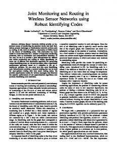
In numerical results section, we let = 1. V. N UMERICAL R ESULTS In this section, the distributed algorithm is simulated over a network that is composed of five sensor nodes and a sink node as shown in Figure 1. The distant between any two adjacent nodes are equal, i.e., dl = d = 50m, l ∈ L. Here, we use the energy dissipation parameters in [15], where εs = 50nJ/bit, εr = 50nJ/bit, μ = 50nJ/bit, η = 0.0013pJ/bit/m4 , and path loss factor n = 4. There are six routes in in Figure 1. These routes are r1 (l1 , l2 ) associated with sensor 1, r2 (l2 ) associated with sensor 2, r3 (l3 , l2 ) associated with sensor 3, r4 (l4 ) associated with sensor 4, r5 (l5 , l4 ) and r6 (l6 , l2 ) associated with sensor 5. For realtime requirement, we give a delay bound vector for the six routes: B = [0.5 0.5 0.5 0.5 0.5 0.5]T . We assume a fixed link capacity cl = 250kbps, l ∈ L, and each node is assumed to have equal initial energy of 5J. The weight wv of each sensor node v is set to 1. Here, we let Uv (sv ) = ln(sv ). Figure 2 presents the convergence property of our algorithm. Here, we set r = 1.0 × 10−17 , β = 5, and we use the constant stepsize α = 0.01, λ = 0.1. Figure 2 shows that dual variables converge fast (after 100 iterations) despite the oscillations at beginning. Figure 3 reconfirms the convergence results of our algorithm. It usually takes more iterations for source rates to converge to the optimal value for given r and β, since the update of source rates takes place in the inner loop. Due to the symmetry in the positions of sensor 1 and sensor 3 with respect to the sink, they have the same optimal dual variables and source rates. Thus, we

978-1-4244-4148-8/09/$25.00 ©2009 This full text paper was peer reviewed at the direction of IEEE Communications Society subject matter experts for publication in the IEEE "GLOBECOM" 2009 proceedings.

0.16

μ1 μ2 μ3 μ4 μ5 μ6

0.14

Dual Variables

0.12 0.1 0.08 0.06 0.04 0.02 0 0

50

100 150 200 Iteration Number

Fig. 2. Fig. 1.

250

300

The evolution of dual variables

The topology of wireless sensor network(5 sensors)

50

VI. C ONCLUSION We have studied the tradeoff between network lifetime and network utility for energy-constrained WSNs with the real-time requirement. Considering rate control and routing under real-time constraints simultaneously, we have derived a distributed algorithm that has been guaranteed to converge

S1 S2 S3 S4 S5

40 Source Rates(kbps)

observe that any two curves associated these two sensors in Figure 2 and Figure 3 coincide with each other . There are two routes originating from sensor node 5. We are curious about how the node 5 distributes its flow between l5 and l6 . In Figure 4, l5 completely dominates the flow generated by node 5, while the flow rate of l6 is nearly zero. The reason is obvious. Node 2 and node 4 are the bottleneck nodes that have the higher power dissipation than the other nodes. Thus, the network lifetime must be the lifetime of node 2 or the lifetime of node 4 according to definition (1). The smart choice made by our algorithm can alleviate the burden of node 2 and balance the flow in the WSN. Figure 5 shows the tradeoff curve between the network utility and network lifetime as the factor r ranges from r = 1.0 × 10−50 to r = 1.0 × 10−25 for β = 10. By increasing r, the network lifetime can be traded for greater network utility through increased source rates. Alternatively, by decreasing r, network utility can be traded for greater network lifetime by reducing the source rates. We observe that when r ≥ 1×10−30 , the tradeoff between network utility and network lifetime is constant. That is due to the fact that some routes are saturated since the real-time constraints can not be violated.

30

20

10

0 0

0.5

Fig. 3.

1 1.5 Iteration Number

2

2.5 4

x 10

The evolution of source rates

to the optimal scheme of the tradeoff model by analysis and simulation. There are several extensions of our work. Future research can be easily extended to the cases of multicommodity flows and multiple sinks. In wireless networks, the link capacity is not fixed any more when transmission scheduling and power assignment are considered. Thus, we will incorporate MAC/Physical layer issues into the lifetime-utility tradeoff framework in future. ACKNOWLEDGMENT The authors would like to thank those anonymous reviewers for their constructive comments and suggestions to

978-1-4244-4148-8/09/$25.00 ©2009 This full text paper was peer reviewed at the direction of IEEE Communications Society subject matter experts for publication in the IEEE "GLOBECOM" 2009 proceedings.

Link Rates (kbps)

80

f1 f2 f3 f4 f5 f6

60

40

20

0 0

0.5

Fig. 4.

1 Iteration Number

1.5

2 4

x 10

The evolution of link rates

55

β=10

r ≥ 1.0e−30 r = 1.0e−31

Network Utility

50

45

40

r = 1.0e−50

35

30 0

0.5

1

1.5

2

Network Lifetime(s)

Fig. 5.

2.5

3

3.5 4

x 10

The network lifetime-utility tradeoff curve

[7] V. Srinivasan, C. L. Chiasserini, P. S. Nuggehalli, and R.R. Rao, ”Optimal rate allocation for energy-efficient multipath routing in wireless ad hoc networks”, IEEE Transactions on Wireless Communications, vol. 3, no. 3, 2004, pp 891-899. [8] Y. T. Hou, Y. Shi, and H. D. Sherali, ”Rate allocation in wireless sensor networks with network lifetime requirement”, in Proc. ACM MobiHoc, 2004, pp 67-77. [9] J. H. Chang and L. Tassiulas, ”Maximum lifetime routing in wireless sensor networks”, IEEE/ACM Transactions on Networking, vol. 12, no. 4, 2004, pp 609-619. [10] R. Madan and S. Lall, ”Distributed algorithms for maximum lifetime routing in wireless sensor networks”, IEEE Transactions on Wireless Communications, vol. 5, no. 8, 2006, pp 2185-2193. [11] J. C. F. Li, S. Dey, and J. Evans, ”Maximal lifetime power and rate allocation for wireless sensor systems with data distortion constraints”, IEEE Transactions on Signal Processing, vol. 56, no. 5, 2008, pp 20762090. [12] H. Nama, M. Chiang, and N. Mandayam, ”Utility-lifetime tradeoff in self-regulating wireless sensor networks: a cross-layer design approach”, in Proc. IEEE ICC, 2006, pp 3511-3516. [13] H. Nama, M. Chiang, and N. Mandayam, ”Optimal utility-lifetime tradeoff in self-regulating wireless sensor networks: a distributed approach”, in Proc. IEEE CISS, 2006, pp 789-794. [14] J. Zhu, K. L. Hung, B. Bensaou, and F. Nait-Abdesselam, ”Tradeoff between network lifetime and fair rate allocation in wireless sensor networks with multi-path routing”, in Proc. ACM/IEEE MSWiM, 2006, pp 301-308. [15] J. Zhu, K. L. Hung, B. Bensaou, and F. Nait-Abdesselam, ”Ratelifetime tradeoff for reliable communication in wireless sensor networks”, Computer Networks, vol. 52, no. 1, 2008, pp 25-43. [16] R. Machado and S. Tekinay, ”A survey of game-theoretic approaches in wireless sensor networks”, Computer Networks, vol. 52, no. 16, 2008, pp 3047-3061. [17] L. Kleinrock, Communication nets: stochastic message flow and delay. New York: McGraw-Hill,1964. [18] J. Mo and J. Walrand, ”Fair end-to-end window-based congestion control”, IEEE/ACM Transactions on Networking, vol. 8, no. 5, 2000, pp 556-567. [19] D. P. Bertsekas, Nonlinear programming. Athena Scientific, 1999. [20] Y. Yao and G. B. Giannakis, ”Energy-efficient scheduling for wireless sensor networks”, IEEE Transactions on Communications, vol. 53, no. 8, 2005, pp 1333-1342.

improve the quality of the paper. R EFERENCES [1] I. F. Akyildiz, W. Su, Y. Sankarasubramaniam, and E. Cayirci, ”Wireless sensor networks: a survey”, Computer Networks, vol. 38, no. 4, 2002, pp 393-422. [2] A. Willig, K. Matheus, and A. Wolisz, ”Wireless technology in industrial networks”, Proceedings of the IEEE, vol. 93, no. 6, 2005, pp 1130-1151. [3] F. Kelly, A. Maulloo, and D. Tan, ”Rate control for communication networks: shadow prices, proportional fairness and stability”, Journal of the Operational Research Society, vol. 49, vol. 3, 1998, 237-252. [4] S. H. Low, and D. E. Lapsley, ”Optimization flow control-I:Basic algorithm and convergence”, IEEE/ACM Transactions on Networking, vol. 7, no. 6, 1999, pp 861-874. [5] F. Kelly and T. Voice, ”Stability of end-to-end algorithms for joint routing and rate control”, ACM SIGCOMM Computer Communication Review, vol. 35, no. 2, 2005, pp 5-12. [6] X. Lin and N. B. Shroff, ”Utility maximization for communication networks with multi-path routing,” IEEE Transactions on Automatic Control, vol. 51, no. 5, 2006, pp 766-781.

978-1-4244-4148-8/09/$25.00 ©2009 This full text paper was peer reviewed at the direction of IEEE Communications Society subject matter experts for publication in the IEEE "GLOBECOM" 2009 proceedings.