Hindawi Wireless Communications and Mobile Computing Volume 2018, Article ID 6261453, 11 pages https://doi.org/10.1155/2018/6261453
Research Article Compressed Sensing Based Joint Rate Allocation and Routing Design in Wireless Sensor Networks Jie Hao 1
,1 Ran Wang,1 Baoxian Zhang
,2 Yi Zhuang
,1 and Bing Chen
1
Nanjing University of Aeronautics and Astronautics, Nanjing, China University of Chinese Academy of Sciences, Beijing, China
2
Correspondence should be addressed to Baoxian Zhang;
[email protected] Received 11 September 2017; Accepted 18 February 2018; Published 27 March 2018 Academic Editor: Paolo Barsocchi Copyright © 2018 Jie Hao et al. This is an open access article distributed under the Creative Commons Attribution License, which permits unrestricted use, distribution, and reproduction in any medium, provided the original work is properly cited. Compressed sensing for wireless sensor networks has attracted a lot of research attention in the last decade for its advantages in energy saving, robustness, and so on. Nevertheless, existing solutions mostly focus on the data compression performance while neglecting the energy efficiency. In this paper, we first present the joint resource allocation problem formulation based on compressed sensing. Then a distributed algorithm to compute the sampling rate and routes utilizing local network status is proposed. We conduct extensive experiments based on meteorological wireless sensor networks to verify the merit of our mechanism; it is shown that the proposed mechanism is able to achieve very high efficiency in terms of network lifetime and sensing quality compared with existing approaches.
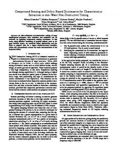
1. Introduction Compressed sensing (CS, also known as compressive sensing) is an efficient tool to process data as it enables sparse sampling while guaranteeing high sampling quality in wireless sensor networks. With CS, the sink node only needs to collect the compressed measurements 𝑦𝑚×1 based on the sensing matrix Φ𝑚×𝑛 instead of the original measurements 𝑥𝑛×1 ; that is, 𝑦𝑚×1 = Φ𝑚×𝑛 𝑥𝑛×1 , 𝑚 < 𝑛. Φ𝑚×𝑛 is generally a Gaussian random matrix in which no entry is zero. The compressed sensing using this kind of nonsparse sensing matrix is referred to as dense compressed sensing. Typically, collection tree is by default used for supporting compressed data collection [1, 2]. Although the network performance is improved somehow, the communication cost needed to collect the compressed measurements caused by dense compressed sensing throughout the network is overlooked. Fortunately, sparse compressed sensing whose sensing matrix is sparse itself can achieve the same compression performance theoretically and experimentally with much less sampling and communication cost [3–6]. Figure 1 shows how sparse CS can reduce the communication consumption compared with dense CS. In this figure, a sensor network consisting of 𝑛 sensor nodes needs to collect all the measurements
from the sensor nodes. Gaussian sensing matrix is used to compress the original measurement and we assume 𝑚 < 𝑛 compressed measurements are required and transmitted to sink by a routing tree. For a single compressed measurement 𝑦𝑗 , that is, the 𝑗th entry of 𝑦𝑚×1 , each node multiplies its own measurement 𝑥𝑖 with 𝜙𝑖𝑗 , adds it with the incoming weighted measurement, and then forwards the added measurement to its next hop until sink receives the compressed measurement 𝑦𝑗 = (𝜙1𝑗 , 𝜙2𝑗 , . . . , 𝜙𝑛𝑗 )(𝑥1 , 𝑥2 , . . . , 𝑥𝑛 )𝑇 . As 𝜙𝑖𝑗 ≠ 0, ∀1 ≤ 𝑖 ≤ 𝑚, 1 ≤ 𝑗 ≤ 𝑛, dense CS implies that each node gets involved in each single compressed measurement. As a result dense CS would generate 𝑂(𝑚𝑛) transmissions in total. In comparison, in sparse CS there is only a single 1 in each row of Φ and 0 elsewhere. It implies only 𝑚 nodes are chosen as the source nodes and hence the total transmission count is 𝑂(𝑚 log 𝑛) as the routing tree depth is 𝑂(log 𝑛). From the temporal perspective, sparse CS indicates each sensor node takes samples under different sampling schedules. Although more energy efficient than dense CS, most literature on sparse CS decouples the sampling and routing design and only concentrates on one side as it assumes either the sampling [5, 6] or the communication energy consumption with energy hungry sensors [3] is neglectable. However, in practice we
2
Wireless Communications and Mobile Computing
1
4 4 4
4 4 4
4 4
Sink Source node Non-source node (a) Dense compressed sensing
1 1 1
3 1
1 Sink Source node Non-source node (b) Sparse compressed sensing
Figure 1: Sparse sampling can reduce the communication cost compared with dense sampling.
observe that the sampling or routing energy consumption could not be neglected in many cases. Take the typical radio module Semtech XE1205 radio transceiver [7] and SHT7x Humidity and Temperature Sensor [8] as examples. The typical TX power is around 62 mA, and the energy consumption for one byte is roughly 22 uJ at 76 kbps. The typical power in humidity measuring status is about 0.55 mA, and it takes a maximum of 20 ms for an 8-bit measurement. Thus the energy consumption for each measurement is 33 uJ. We can see that neither energy consumption for sampling nor routing should be ignored in this case for energy efficiency optimization. Therefore, this paper considers both sampling and routing energy consumption and aims at finding a joint design mechanism based on CS entitled Distributed Sampling Rate and Routing (DSRR) mechanism to optimize the overall energy consumption. The main contributions of this paper are summarized as follows: (i) We formulate a compressed sensing based joint design problem that tackles sampling and routing simultaneously. (ii) We propose a distributed algorithm that only utilizes local network status to achieve prolonged network lifetime and high sensing quality. (iii) We conduct extensive experiments based on real data set and network deployment from SensorScope [9], which demonstrate the effectiveness of the proposed joint design. The rest of this paper is organized as follows. A literature review of existing work is presented in Section 2. Section 3 describes the a priori knowledge of compressed sensing followed by Section 4 that presents compressed sensing based joint design formulation and the distributed algorithm. Section 5 reports our experimental results. Finally we make a conclusion in Section 6.
for data compression. CDG (Compressive Data Gathering) [10] utilizes spatial correlation and uses CS for snapshot data gathering. Ji et al. [12] explore CS for both snapshot and continuous data gathering under channel interference model. Other than reducing the measurements, some research work explores the impact of routing on the CS performance. Quer et al. [1] combined geographical routing with CS and were surprised to observe that CS is not as good as expected. Luo et al. [2] explore the network throughput of tree based CS and conclude that the hybrid manner that only uses CS near the root of the tree can achieve higher throughput than pure CS. Lee et al. [4] employ CS on shortest path tree based cluster structure. In the above research work, although the collected measurements using CS are significantly reduced, all the sensor nodes must be involved in each single measurement. This kind of CS mechanism is catalogued to dense CS. Dense CS focuses on minimizing the number of measurements rather than the communication cost and sampling cost. Therefore, a rich body of literature aims to address the communication cost optimization and sampling cost optimization issue with CS. Fortunately, sparse sensing matrix is proved to have the same compression performance theoretically and experimentally [3, 5, 6]. In sparse CS, each row of sensing matrix requires 𝑂(log 𝑛) nonzero entries in [14] or only one nonzero entry in [3, 5, 15]. In sparse CS, collection tree is usually adopted for routing to gather the sparse measurements. Wang et al. [14] choose randomly 𝑚 projection nodes in charge of collecting data from nonprojection nodes and sink only needs to query the projection nodes for data reconstruction. Shen et al. [6] use ETX routing metric to determine the sampling rate of each node; that is, lower ETX nodes have more opportunity to take samples. This nonuniform sampling can achieve the same sensing accuracy with less energy consumption. Chou et al. [16] aim at finding the sensing matrix that maximizes information gain to energy expenditure. It decouples the sensing matrix setting problem into two subproblems, location of nonzero elements (i.e., the routing), and the values of the nonzero elements in the sensing matrix. Rana et al. [3] notice that the energy consumption for sampling is much higher than communication for energy hungry sensors such as wind speed sensor and thus adapts the sample rates according to the harvest energy. Though energy efficient considering sampling consumption, [3] does not consider the routing issue. From the literature review, we can see that most research works neglect either energy consumption for sampling or communication. More specifically, they focus on either sampling scheduling or routing design. In comparison, our work in this paper considers both energy consumption for sampling and communication and thus jointly optimizes both sampling and routing design.
2. Related Work The research concerning CS can be traced back to the last decade. Shortly after its invention, CS was introduced into wireless sensor networks for its advantages in energy conservation, transmission robustness, and so on [10–13]. At the very beginning, the literature mainly focused on using CS
3. A Priori Knowledge on CS This section will illustrate the a priori knowledge of compressed sensing used in our paper. Given a sensor network 𝐺(𝑉, 𝐿), where 𝑉 is the vertex set and 𝐿 is the link set, respectively, 𝑛 and 𝑙 are the cardinalities of 𝑉 and 𝐿. The data
Wireless Communications and Mobile Computing
3
from all the nodes form a data vector 𝑥 = [𝑥1 , 𝑥2 , . . . , 𝑥𝑛 ]𝑇 . If 𝑥 can be projected into a sparse signal 𝑠 with representation basis Ψ, that is, 𝑥 = Ψ𝑠, the original data 𝑥𝑛×1 can be compressed to 𝑦𝑚×1 , 𝑚 < 𝑛 by sensing matrix Φ𝑚×𝑛 ; that is, we have 𝑦 = Φ𝑥 = ΦΨ𝑠.
(1)
The reconstructed data 𝑥̂ is obtained by 𝑥̂ = Ψ̂𝑠, where 𝑠̂ is the optimal solution of min s.t.
‖𝑠‖𝑙0 , 𝑦 = ΦΨ𝑠,
(2)
or alternatively min s.t.
‖𝑠‖𝑙1 , 𝑦 = ΦΨ𝑠,
‖𝑥̂ − 𝑥‖2 . ‖𝑥‖2
4.1. Energy Consumption Model. Given a sensor network consisting of 𝑛 sensor nodes, the energy consumption of a sensor node 𝑖, ec𝑖 , mainly includes the energy consumption for 𝑖 𝑖 , communication 𝐸comm , computation sampling (sensing) 𝐸sp 𝑖 𝑖 𝑖 𝑖 + 𝐸comp + 𝐸comp , and status switching 𝐸sw ; that is, ec𝑖 = 𝐸sp 𝑖 𝑖 𝑖 𝑖 𝐸sw + 𝐸comm [19]. Among all the consumption, 𝐸comp and 𝐸sw 𝑖 𝑖 can be usually neglected compared with 𝐸sp and 𝐸comm . Thus, the equation is rewritten as 𝑖 𝑖 + 𝐸comm . ec𝑖 ≈ 𝐸sp
(3)
to reduce complexity. Two performance metrics involved in compressed sensing are CR (Compression Ratio), defined as CR = 𝑚/𝑛, and the reconstruction error defined as 𝜖=
sacrificing sensing quality. To this end, we firstly illustrate the energy consumption model of the network in Section 4.1 and present the joint design formulation in Section 4.2 and the distributed algorithm in Section 4.3.
(4)
With compressed sensing, the sensor nodes take measurements at a low sampling rate without significant information degradation. Specifically, Φ𝑚×𝑛 specifies a sampling policy: each sensor node can only take one measurement at any scheduled time slot upon actuation; if the 𝑖th measurement is taken at time slot 𝑗, Φ𝑚×𝑛 has 1 in the (𝑖, 𝑗) position (1 ≤ 𝑖 ≤ 𝑚, 1 ≤ 𝑗 ≤ 𝑛), that is, 𝜙𝑖𝑗 = 1. The resulting sensing matrix Φ is sparse as it contains only one 1 element in any row, at most one 1 in any column, and 0 everywhere else. Given a sampling rate 𝑟 for a sensor node, 𝑚 = ⌊𝑛𝑟⌋ measurements should be taken and the positions of the nonzero entries are randomly chosen. To reconstruct the original data, representation basis Ψ and recovery algorithm need to be dedicatedly designed. The choice of Ψ should satisfy two main criteria. Firstly, Ψ should transform 𝑥 into a sufficiently sparse signal in some domain. In the other words, 𝑠 = Ψ−1 𝑥 should be as sparse as possible. Secondly, Ψ should be sufficiently incoherent with Φ. A rich body of literature has provided us with many good choices. DCT, Haar, wavelet transformation, differential matrix, and so on are widely used as representation basis. In particular, DCT, Haar, and so on are superior to differential matrix in terms of sparsity while differential matrix performs better regarding incoherence with the sparse sensing matrix [15]. BP, OMP, SL0, and so on as the recovery algorithm [17, 18] are widely used. In this paper, we will choose the exact CS method based on field data in the performance evaluation in Section 5.
4. Joint Design of Sampling and Routing This paper aims to present a joint design of sampling and routing that can achieve prolonged network lifetime without
(5)
𝑖 𝑖 Now we investigate 𝐸sp and 𝐸comm in detail. The former 𝑖 one 𝐸sp is proportional to the number of samples that node 𝑖 is proportional to the active time of the radio 𝑖 takes. 𝐸comm for transmission, reception, and idle listening. In this paper, we assume each sensor node is fully aware of when it should be turned on to receive and transmit according to our joint 𝑖 only considers optimized design. Thus, in our model, 𝐸comm energy consumption for transmitting and receiving. Let 𝑒sp be the energy consumption for sampling once. We can obtain 𝑖 = 𝑒sp 𝑟𝑖 . 𝐸sp
(6)
Let 𝑒𝑡𝑥 and 𝑒𝑟𝑥 be the energy consumption for transmitting and receiving, respectively, 𝐹 = {𝑓𝑖𝑗 , ∀𝑖 ∈ 𝑉 & 𝑗 ∈ 𝑁𝑖 } be the flow from node 𝑖 to 𝑗 belonging to 𝑖’s neighbor set 𝑁𝑖 . We have 𝑖 𝐸comm ≈ 𝑒𝑡𝑥 ∑ 𝑓𝑖𝑗 + 𝑒𝑟𝑥 ∑ 𝑓𝑗𝑖 . 𝑗∈𝑁𝑖
𝑗∈𝑁𝑖
(7)
4.2. Problem Formulation. Before we proceed to the specifics, we list all the involved notations and their semantics in Notations. Given a sensor network 𝐺(𝑉, 𝐿), during its lifetime 𝑇, each node samples the target phenomenon at a low rate and transmits the samples to a sink node by multihop routing. Assume the application requires an overall sampling rate 𝑟0 to achieve desired sensing quality. Network lifetime is defined as the minimum node lifetime among all the nodes in the network. We aim at designing the sampling and routing schedule jointly to maximize the network lifetime under the desired sampling rate constraint. Therefore, the joint design problem can be formulated as max r,f
s.t.
𝑇,
(8)
𝑟𝑖 ≤ ∑ 𝑓𝑖𝑗 − ∑ 𝑓𝑗𝑖 , 𝑗∈𝑁𝑖
ec𝑖 𝑇 ≤ 𝐸𝑖 ,
∀𝑖 ∈ [1, 𝑛] ,
𝑗∈𝑁𝑖
∀𝑖 ∈ [1, 𝑛] ,
(9) (10)
𝑛
𝑟0 𝑛 ≤ ∑𝑟𝑖 . 𝑖=1
(11)
4
Wireless Communications and Mobile Computing
Condition (9) is the flow conservation constraint; (10) is the energy constraint where ec𝑖 = 𝑒𝑡𝑥 ∑ 𝑓𝑖𝑗 + 𝑒sp 𝑟𝑖 + 𝑒𝑟𝑥 ∑ 𝑓𝑗𝑖 , 𝑗∈𝑁𝑖
𝑗∈𝑁𝑖
(12)
and (11) guarantees that the average sampling rate is higher than 𝑟0 . Replacing 𝑇 by 1/𝑞, we create an equivalent problem min 𝑞2 ,
(13)
ec𝑖 ≤ 𝐸𝑖 𝑞, ∀𝑖 ∈ [1, 𝑛] .
(14)
𝑟,𝑓
and (10) becomes
Moreover, we also hope to maximize the fairness of the sampling rates among all the nodes; that is, the variance of the sampling rates ∑𝑛𝑖=1 (𝑟𝑖 − 𝑟0 )2 which is convex should be minimized. In this way, we hope to avoid the case that the optimization may lead to zero measurement for a traffic heavy node and thus incurs high data loss if spatial correlation is not sufficiently high. To this end, we add a regularization term in our joint design objective (13) as follows: 𝑛
2
min 𝑞2 + Θ∑ (𝑟𝑖 − 𝑟0 ) , 𝑟,𝑓
(15)
𝑖=1
where Θ is the regularization parameter that pursues performance balance between network lifetime and fairness. The optimization problem can be easily solved in a centralized way. However, a centralized algorithm in wireless sensor networks is impractical since it requires overwhelming high communication or computation overhead. In this case, in order to carry out the optimization in resource limited wireless sensor networks with lower communication/computation overhead, we propose a distributed algorithm in the following subsection. 4.3. Distributed Sampling Rate and Routing Mechanism. Based on the problem formulation in the last subsection, we propose a distributed algorithm entitled Distributed Sampling Rate and Routing (DSRR) mechanism that can solve the problem by using only local network status. In order to perform the optimization fully distributively, we reformulate the problem to a convex quadratic optimization problem: 𝑛
𝑛
𝑖=1
𝑖=1
2
min ∑𝑞𝑖2 + Θ∑ (𝑟𝑖 − 𝑟0 ) , r,f
s.t.
(9) , (14) , (11) 𝑞𝑖 = 𝑞𝑗 , ∀𝑖, 𝑗 ∈ [1, 𝑛] .
(16)
(17)
Now, we form the Lagrangian by introducing Lagrangian multipliers 𝜆, 𝜂, 𝜉, and 𝜌 for the constraints, respectively.
𝐿 (𝑞, 𝑓, 𝑟, 𝜂, 𝜆, 𝜉, 𝜌) 𝑛
2
𝑛
𝑛
= ∑ 𝑞𝑖2 + Θ ∑ (𝑟𝑖 − 𝑟0 ) + ∑ 𝛾𝑖 [𝑟𝑖 − ∑ (𝑓𝑖𝑗 − 𝑓𝑗𝑖 )] + ∑ ∑ 𝜆 𝑖𝑗 (𝑞𝑖 − 𝑞𝑗 ) + ∑𝜂𝑖 (𝑟0 − 𝑟𝑖 ) + ∑ ∑ 𝜉𝑖𝑗 (𝜂𝑖 − 𝜂𝑗 ) + ∑ 𝜌𝑖 (ec𝑖 − 𝐸𝑖 𝑞𝑖 ) 𝑗∈𝑁𝑖 𝑖=1 𝑖=1 𝑗=1 𝑖∈[1,𝑛] 𝑖∈[1,𝑛] 𝑖∈[1,𝑛] 𝑖∈[1,𝑛] ] 𝑖∈[1,𝑛] 𝑗∈𝑁𝑖 [ } { 2 = ∑ {𝑞𝑖2 + 𝑞𝑖 ∑ (𝜆 𝑖𝑗 − 𝜆 𝑗𝑖 ) − 𝜌𝑖 𝐸𝑖 𝑞𝑖 + Θ (𝑟𝑖 − 𝑟0 ) + 𝛾𝑖 𝑟𝑖 − 𝑟𝑖 𝜂𝑖 + 𝜌𝑖 𝑒sp 𝑟𝑖 + ∑ [(𝜌𝑖 𝑒𝑡𝑥 − 𝛾𝑖 ) 𝑓𝑖𝑗 + (𝜌𝑖 𝑒𝑟𝑥 + 𝛾𝑖 ) 𝑓𝑗𝑖 ] + 𝜂𝑖 (𝑟0 + ∑ (𝜉𝑖𝑗 − 𝜉𝑗𝑖 ))} 𝑗∈𝑁𝑖 𝑗∈𝑁𝑖 𝑗∈𝑁𝑖 𝑖∈[1,𝑛] } {
(18)
s.t. 𝑓 ∈ Ω𝑓 , 𝑟 ∈ Ω𝑟 , 𝑞 ∈ Ω𝑞 ,
where Ω𝑓 , Ω𝑟 , and Ω𝑞 are feasible regions. We fix dual variables and then define subproblems and master problem as follows. The subproblems include
min s.t. min
{ } ∑ {𝑞𝑖2 + 𝑞𝑖 ∑ (𝜆 𝑖𝑗 − 𝜆 𝑗𝑖 ) − 𝜌𝑖 𝐸𝑖 𝑞𝑖 } , 𝑗∈𝑁𝑖 𝑖∈[1,𝑛] { } 𝑞 ∈ Ω𝑞 ,
s.t.
(21)
𝑓 ∈ Ω𝑓 ,
with optimal values 𝑔𝑟 (𝜌), 𝑔𝑞 (𝜌), 𝑔𝑓 (𝜌), respectively. The master problem is 𝑔𝑟 (𝜌) + 𝑔𝑞 (𝜌) + 𝑔𝑓 (𝜌) and 𝜌𝑖 is updated as
𝑢𝑖(𝑡)
∑ {Θ (𝑟𝑖 − 𝑟0 ) + 𝛾𝑖 𝑟𝑖 − 𝑟𝑖 𝜂𝑖 + 𝜌𝑖 𝑒sp 𝑟𝑖 } ,
𝑟 ∈ Ω𝑟 ,
∑ ∑ (𝜌𝑖 𝑒𝑡𝑥 − 𝛾𝑖 ) 𝑓𝑖𝑗 + (𝜌𝑖 𝑒𝑟𝑥 + 𝛾𝑖 ) 𝑓𝑗𝑖 ,
𝑖∈[1,𝑛] 𝑗∈𝑁𝑖
𝜌𝑖(𝑡+1) = max {𝜌𝑖(𝑡) + 𝛼𝑡 𝑢𝑖(𝑡) , 0} , 2
𝑖∈[1,𝑛]
s.t.
(19)
min
(20)
(22)
= ec𝑖 − 𝐸𝑖 𝑞𝑖 ,
where 𝛼𝑡 is the update stepsize. The optimal value 𝑔𝑞 (𝜌) 𝑔𝑟 (𝜌) can be obtained distributively at each node with
Wireless Communications and Mobile Computing
5
Distributed Sampling Rate & Routing control mechanism At each iteration, do Sink broadcasts a Route Request (RREQ) message containing its cost with 𝐶sink = 0 and its 𝑞, 𝜂. Upon receiving the RREQ from its neighbors within its deferring time, a sensor node 𝑖 updates its cost as 𝐶𝑖 = min{(𝜌𝑖 𝑒𝑡𝑥 − 𝛾𝑖 ) + (𝜌𝑗 𝑒𝑟𝑥 + 𝛾𝑗 ) + 𝐶𝑗 , ∀𝑗 ∈ 𝑁𝑖 }, chooses the neighbour node leading to 𝐶𝑖 as its parent node. 𝑖 keeps overhearing all its neighbours and updates the Lagrange multipliers 𝜂, 𝛾, 𝜆, 𝜉, 𝜌 according to (22) (24) (23). Node 𝑖 distributively computes 𝑟𝑖∗ , 𝑞𝑖∗ . Node 𝑖 arranges its RREQ and broadcast to its neighbors. This procedure continues until all nodes determine their parent nodes, sampling rates, and update their parameters. Every sensor node executes the obtained sampling rate, routing, and recodes its input/output traffic flow. end Algorithm 1: Working process of DSRR.
100
Objective function
𝑞𝑖∗ = (𝜌𝑖 𝐸𝑖 − ∑𝑗∈𝑁𝑖 (𝜆 𝑖𝑗 − 𝜆 𝑗𝑖 ))/2 and 𝑟𝑖∗ = (2Θ𝑟0 + 𝜂𝑖 − 𝛾𝑖 − 𝜌𝑖 𝑒sp )/2Θ, respectively. 𝑔𝑓 (𝜌) can be solved with global (or end-to-end) network information in polynomial time. In this paper, we aim at solving (21) by building a minimum cost tree. Observe that, in order to minimize (21), the traffic flow is encouraged to be routed along the path which produces the lowest ∑𝑖∈[1,𝑛] ∑𝑗∈𝑁𝑖 (𝜌𝑖 𝑒𝑡𝑥 − 𝛾𝑖 )𝑓𝑖𝑗 + (𝜌𝑖 𝑒𝑟𝑥 + 𝛾𝑖 )𝑓𝑗𝑖 . With this motivation, we design the distributed routing mechanism as follows. The cost function of each link (𝑖𝑗) is defined as 𝑐𝑖𝑗 = (𝜌𝑖 𝑒𝑡𝑥 − 𝛾𝑖 ) + (𝜌𝑗 𝑒𝑟𝑥 + 𝛾𝑗 ), ∀𝑖 ∈ [1, 𝑛], 𝑗 ∈ 𝑁𝑖 . Starting from the sink node, each node 𝑖 updates its cost as 𝐶𝑖 = min{𝑐𝑖𝑗 +𝐶𝑗 , ∀𝑗 ∈ 𝑁𝑖 } and chooses the neighbor node leading to 𝐶𝑖 as its parent node 𝑝𝑖 . This procedure continues until all nodes update their costs and decide their parents. In this way, the tree minimizing (21) is established. Please note that the other Lagrange multipliers are updated as
10−2
10−4
0
100
200 300 Iterations
400
500
DSRR OPT
Figure 2: The convergence time of DSRR.
𝛾𝑖(𝑡+1) = max (0, 𝛾𝑖(𝑡) + 𝛼𝑡 𝑢𝑖(𝑡) ) , (𝑡) = 𝜆(𝑡) 𝜆(𝑡+1) 𝑖𝑗 𝑖𝑗 + 𝛼𝑡 V𝑖𝑗 ,
𝜂𝑖(𝑡+1) = max (0, 𝜂𝑖(𝑡) + 𝛼𝑡 𝑤𝑖(𝑡) ) ,
(23)
𝜉𝑖𝑗(𝑡+1) = 𝜉𝑖𝑗(𝑡) + 𝛼𝑡 ℎ𝑖(𝑡) , where 𝑢𝑖(𝑡) , V𝑖𝑗(𝑡) , 𝑤𝑖(𝑡) , and ℎ𝑖(𝑡) are the components of the (𝑡) (𝑡) subgradient of 𝐿 evaluated at 𝛾𝑖(𝑡) , 𝜆(𝑡) 𝑖𝑗 , 𝜂𝑖 , and 𝜉𝑖𝑗 and can be obtained by
𝑢𝑖(𝑡) = 𝑟𝑖 − ∑ (𝑓𝑖𝑗 − 𝑓𝑗𝑖 ) , 𝑗∈𝑁𝑖
V𝑖𝑗(𝑡) = 𝑞𝑖 − 𝑞𝑗 , 𝑤𝑖(𝑡) = 𝑟0 − 𝑟𝑖 + ∑ (𝜉𝑖𝑗 − 𝜉𝑗𝑖 ) , 𝑗∈𝑁𝑖
ℎ𝑖(𝑡) = 𝜂𝑖 − 𝜂𝑗 .
(24)
The overall Distributed Sampling Rate and Routing (DSRR) control mechanism is summarized in Algorithm 1. DSRR needs to carry out message exchange for multiplier update before its convergence. The overhead of DSRR is approximately proportional to the convergence iteration and also the message exchanging overhead for each iteration. Figure 2 shows the convergence time of DSRR with a Great St. Bernard Pass network whose detailed description can be found in Section 5. We can see that DSRR is able to converge in about 110 iterations which means DSRR requires about 110 rounds of network-wide information exchange before it works with the optimized sampling rate and routing decision. In each iteration, DSRR works similar to the classic OnDemand Distance Vector (AODV) Routing and its variants [20, 21]. In a path discovery process by DSRR, a Route Request (RREQ) message needs to carry the following information: one kind is local Lagrangian multiplier updating related information to be exchanged within neighborhood, including 𝑞𝑗 needed by 𝜆 𝑖𝑗 and 𝜂𝑗 needed by 𝜉𝑖𝑗 ; the other kind is cost of
6
Wireless Communications and Mobile Computing
5.805
×105
1.527
×105
5.795
8 2 3
10 6
7 15 2014 12
13 11
5
9
19
17 18
4
5.79 5.785 32
5.78
28
31 29
25
Nord (m) in Coordinate CH1903
Nord (m) in Coordinate CH1903
1.5265 5.8
1.526 1.5255 1.525
201 63 202 203 47 207 7 27 204 206 99 111 75 64 61 71 65
1.5245
11
51
1.524 1.5235
84 103
81
87 109
1.5225
7.97
7.98 7.99 8 8.01 8.02 Est (m) in Coordinate CH1903
8.03 ×10⁴
1.522 5.3295
122 68 70 72 49 55 66 54 73
80 96
1.523
5.33
60 10732 31 69 94 3550 19 92 100 33 97 53 10
95 79 93
104
85 89
5.775 7.96
23 423 5 17 9 37 36 26 30 21 46 8 18 121 15 4445 12 25 391424 41 56 105 13 43 59 40 34 57 106 82 62 76
88
98
5.3305 5.331 5.3315 5.332 Est (m) in Coordinate CH1903
(a) Great St. Bernard Pass
5.3325
5.333 ×10⁵
(b) LUCE
Figure 3: Network layout.
the path found so far, which records the cost of the path from the sink to the sender 𝑖 of the received RREQ, that is, 𝐶𝑖 . In addition, in order to minimize the communication overhead for path discovery, we can arrange the travelling speed of RREQ message across the network by introducing intentional deferring at intermediate nodes. For this purpose, we can set the deferring time of a received RREQ at an intermediate node to be proportional to the cost of the link over which the message was received and accordingly initiates a deferred timer. Once expired, the RREQ will be rebroadcasted. In case a new RREQ received from another neighbor leads to a shorter path cost, the path cost will be updated and the timer will be shortened. The node will record the neighbor which sends it the RREQ leading to the least cost as its parent node for it to deliver sensing data to sink later. After retransmitting the RREQ, a node will not need to process any duplicate RREQs further. In this way, each intermediate node only needs to retransmit the RREQ once and thus the communication overhead for route discovery is minimized as 𝑂(𝑛). Therefore, the communication complexity of DSRR is overall 𝑂(𝑛).
5. Evaluation We conduct experiments to evaluate the proposed joint design using field data. SensorScope [9] is a turnkey solution for environmental monitoring systems, based on a wireless sensor network and resulting from a collaboration between environmental and network researchers. The sensors periodically sample the environment and transmit their readings through the wireless network to a sink. Specifically, we use two networks for our evaluation. One is deployed in Great St. Bernard Pass between Switzerland and Italy as a typical small scale network. The other is LUCE (Lausanne Urban Canopy Experiment) as a network of medium size. The following is the detailed experimental setting.
5.1. Experimental Setting Network Setting. The network topologies of Great St. Bernard and LUCE are shown in Figures 3(a) and 3(b), respectively, where we assume a virtual node sitting between nodes 4 and 32 as the sink node in Great St. Bernard Pass network and a node near 68 as the sink node in LUCE network. The initial energy of the nodes is randomly chosen in the order of 30 kJ. In addition, as we notice that the value of the objective function would be extremely trivial with the experimental setting, we rescale the initial energy of each node by multiplying 10−5 and readjust the resulting network lifetime by multiplying 105 . In SensorScope, the meteorological phenomenon such as ambient temperature, surface temperature, and relative humidity are sampled every 2 minutes. Thus, we set a time slot of 2-minute length and evaluate the network lifetime in the unit of time slot. The network parameters involved are illustrated as follows. Radio Transceiver. SensorScope uses Semtech XE1205 radio transceiver [7] with a transmission rate of 76 Kbps [9]. Its transmitting/receiving power is 31 mA (at 5 dBm) and 14 mA, respectively. We assume the packet size is constantly 2 bytes so that the energy consumption for a packet transmitting and receiving is roughly 21.54 uJ and 9.73 uJ, respectively. Sensors. Sensirion SHT75 [8] is adopted for air temperature and humidity. Power consumption for measuring is typically 0.55 mA (we neglect the power consumption 5 𝜇W for sleeping). It usually takes about 20 ms for an 8-bit measurement. Therefore, the energy consumed by a sample is regulated at roughly 𝑒sp = 36.3 uJ. The values of the involving parameters regarding energy consumption are summarized in Table 1.
7
100
100
10−1
10−1
Reconstruction error
Reconstruction error
Wireless Communications and Mobile Computing
10−2
10−3
10−4
0
0.2
0.4 Desired rate
0.6
0.8
10−2
10−3
10−4
DiffM + BP DCT + BP
DiffM + SL0 DCT + SL0
0
0.2
Reconstruction error
0.6
0.8
DiffM + BP DCT + BP
DiffM + SL0 DCT + SL0
(a) Ambient temperature
10
0.4 Desired rate
(b) Surface temperature
0
10−2
10−4
10−6
0
0.2
0.4 Desired rate
0.6
0.8
DiffM + BP DCT + BP
DiffM + SL0 DCT + SL0 (c) Soil moisture
Figure 4: Reconstruction error 𝜖 under different CS methods.
Table 1: Network parameters. 𝑒sp 36.3 uJ
𝑒𝑡𝑥 21.54 uJ
𝑒𝑟𝑥 9.73 uJ
5.2. Network Configuration. In this subsection we configure the parameters involved in the design, including CS method and Θ. 5.2.1. CS Method Selection. In this subsection, we will choose the CS method which is suitable for our experimental data by evaluation. We utilize the measurements sampled by one sensor node as the data input. Figure 4 shows the reconstruction error with different CS methods, where the sensing matrix Φ is always the sparse matrix generated
by the uniform sampling and Ψ−1 could be DCT, Haar, DFT, and Difference Matrix (DiffM in short); the recovery algorithm could be Basis Pursuit (BP) or SL0. From the experiment results we can draw the same conclusion that DiffM performs superior to the others regarding three types of meteorological data. Due to the space limitation, we only show the comparison results of DCT, DiffM and BP, SL0 combination in Figure 4 with respect to three types of meteorological data. Considering SL0 is computationally faster than BP, we choose the combination of sparse sensing matrix, DiffM and SL0 as the CS method hereafter. 5.2.2. The Impact of Θ. Our joint design aims at achieving a good balance between the lifetime and fairness among sampling rates which is tuned by the regularization parameter Θ. Please note that we use the variance of the sampling rate
8
Wireless Communications and Mobile Computing
9
×108 2.5
×10−3
8.8 2
8.4
Variance
Lifetime
8.6
8.2
1.5 1
8 0.5
7.8 7.6
0
1
102
10
103
104
0
105
0
1
10
(a) Lifetime
102
103
104
105
104
105
(b) Variance
Figure 5: Performance with varying 𝜃 of the Great St. Bernard network. ×108 0.025
6.8
0.02
6.6
0.015
Variance
Lifetime
7
6.4 6.2 6
0.01 0.005
0
1
10
102
103
104
105
(a) Lifetime
0
0
1
10
102
103
(b) Variance
Figure 6: Performance with varying 𝜃 of the LUCE network.
vector [𝑟1 , 𝑟2 , . . . , 𝑟𝑛 ] as the indicator of the fairness among sampling rates; that is, the lower the variance, the higher the fairness. Thus, we determine Θ by using the benchmark design OPT, in which the sampling rate and routing are obtained by solving the optimization (16) with CVX tool [22]. OPT works as a benchmark for evaluation and provides us with the guidance for network configuration. We observe that the setting of Θ should be relevant with the value of ∑𝑛𝑖=1 𝑞𝑖2 , where 𝑞 should be proportionate to the traffic load 𝑛𝑟0 and inversely proportional to network density 𝐷 and the energy capacity order 𝐸. Thus we intuitively design Θ = 𝜃 × (𝑛𝑟0 /(𝐷𝐸))2 and explore the impact of 𝜃 on the optimization problem. From Figures 5 and 6, we can observe that with higher 𝜃 the joint design prefers to pursue fairness (i.e., low variance of the sampling rates of the nodes) rather than prolonged network lifetime and DSRR degrades to uniform sampling and network maximization routing with extremely
high 𝜃. In order to achieve the performance balance, we prefer 𝜃 = 10 in the following experiments. 5.3. Lifetime and Sensing Quality. This subsection evaluates the lifetime and reconstruction error performance of DSRR compared with three other mechanisms. One is used in SensorScope [9] combining uniform sampling and energy-aware anypath routing, referred to as USAR in this paper. Specifically, uniform sampling means all nodes share the same sampling rate and energy-aware anypath routing means each node in the network randomly chooses one among maximally three energy richest neighbors with less hop distance to the sink as its parent node on the routing tree. The second one is energy-aware sampling and anypath routing design referred to as EASAR in this paper where energy-aware sampling means each node adjusts its sampling rate proportional to its available energy [3]
Wireless Communications and Mobile Computing
2
9
×109 0.01
×108 1.6
0.008
1.4
Reconstruction error
Lifetime (slots)
1.5
1.2 1
1
0.39
0.4
0.41
0.5
0
0.006
0.004
0.002
0
0.2
0.4 0.6 Desired rate
0.8
0
1
0
OPT DSRR
USAR EASAR
0.2
0.4 0.6 Desired rate
USAR EASAR
0.8
1
OPT DSRR
(b) Reconstruction error 𝜖
(a) Lifetime
Figure 7: Performance with varying 𝑟0 of the Great St. Bernard Pass network. ×108
12
2.5
2.2
10 Lifetime (slots)
0.01
×108
2
8
0.39
6
0.4
0.41
4
1.5 0.35 0.4 0.45
0.006
0.004
0.002
2 0
×10−3
2
0.008
2.1
Reconstruction error
14
0
0.2
0.4 0.6 Desired rate
USAR EASAR
0.8
1
OPT DSRR (a) Lifetime
0
0
0.2
0.4 0.6 Desired rate
USAR EASAR
0.8
1
OPT DSRR
(b) Reconstruction error 𝜖
Figure 8: Performance with varying 𝑟0 of the LUCE network.
while maintaining the overall required sampling rate by CS. Although the two schemes take energy conservation into account in the sampling policy and routing design, they do not fully take advantage of the coupling of sampling and routing based on CS. The last one is the centralized design OPT as described in Section 5.2.2. The comparison results are shown in Figures 7 and 8. Given Figures 7(a) and 8(a), obviously the proposed DSRR performs superior to USAR and EASAR significantly in terms of network lifetime. Both USAR and EASAR are supposed to have good performance in the scenario that 𝑒sp is
much higher than 𝑒𝑡𝑥 and 𝑒𝑟𝑥 . However, in our experimental setting, the energy consumption of sampling is comparable with that of communication. In this case, the joint design DSRR achieves prolonged lifetime because it jointly optimizes the sampling and routing, whereas DSRR is highly superior to USAR and EASAR at a very low sampling rate 𝑟0 = 0.1, and the difference among all the schemes decreases as 𝑟0 increases. This is because, with higher sampling rate, the sampling rate and route diversity generated by the schemes are becoming low so that the gain of DSRR beyond the others saturates.
10
Wireless Communications and Mobile Computing
Figures 7(b) and 8(b) show the reconstruction error with increasing 𝑟0 . (As there exists data error regarding LUCE network, we remove all measurements from abnormal sensor nodes.) We can see that overall uniform sampling in USAR performs best among all the schemes. The result conforms to our expectation that uniform sampling would conserve more spatial correlation and thus lead to less reconstruction error. Although DSRR results in higher reconstruction error, the reconstruction error of DSRR stays lower than 0.01 which is sufficiently low compared with the state of the art [15, 23]. In this experiment, we only use the ambient temperature data for evaluation. Similar results based on surface temperature and soil moisture data are omitted in this paper. In summary, Figures 7 and 8 verify that DSRR can achieve prolonged network lifetime with little sensing quality degradation compared with existing work. From the evaluation for Great St. Bernard Pass network and LUCE network, we can draw a conclusion that, for both small scale networks and medium scale networks, the centralized solution OPT and the proposed DSRR perform superior to the other existing mechanisms.
6. Conclusions In this paper, we explore the advantage of CS in the joint design of sampling and routing. We formulate a CS based optimization model to prolong network lifetime and guarantee sensing quality simultaneously and then propose a distributed algorithm DSRR that only requires local network status to achieve global network performance improvement. We conduct extensive experiments based on environmental network topologies and data. The experiment results demonstrate that the centralized algorithm and the distributed algorithm can achieve prolonged network lifetime with unnoticeable sensing quality sacrifice for both small scale and medium scale sensor networks compared with existing research work. The proposed algorithm is suitable for sensor networks with data correlation, such as meteorological sensor networks of different network size. As part of our future work, we will employ energy profile prediction model to further improve the efficiency of our joint design.
Notations 𝑛: 𝑇: 𝑁𝑖 : 𝑟𝑖 : 𝑟0 : 𝑓𝑖𝑗 : ec𝑖 : 𝐸𝑖 :
Network size Network lifetime The neighbor set of node 𝑖 Sampling rate of 𝑖 Required sampling rate by CS Flow on link (𝑖, 𝑗) Energy consumption rate of 𝑖 Initial energy capacity of 𝑖.
Disclosure Any opinions, findings, and conclusions or recommendations expressed in this material are those of the authors and do not necessarily reflect the views of the funding agencies.
Conflicts of Interest The authors declare that there are no conflicts of interest regarding the publication of this paper.
Acknowledgments This work was supported in part by National Natural Science Foundation of China under Grants 61602242 and 61602238, Natural Science Foundation of Jiangsu Province under Grants BK20160807, BK20160812, and BK20160805, and Research Funding 2016-PYS/K-KY-J061.
References [1] G. Quer, R. Masiero, D. Munaretto, M. Rossi, J. Widmer, and M. Zorzi, “On the interplay between routing and signal representation for compressive sensing in wireless sensor networks,” in Proceedings of the Information Theory and Applications Workshop (ITA ’09), pp. 206–215, IEEE, San Diego, Calif, USA, February 2009. [2] J. Luo, L. Xiang, and C. Rosenberg, “Does compressed sensing improve the throughput of wireless sensor networks?” in Proceedings of the IEEE International Conference on Communications (ICC ’10), pp. 1–6, IEEE, May 2010. [3] R. Rana, W. Hu, and C. T. Chou, “Energy-aware sparse approximation technique (EAST) for rechargeable wireless sensor networks,” Lecture Notes in Computer Science (including subseries Lecture Notes in Artificial Intelligence and Lecture Notes in Bioinformatics): Preface, vol. 5970, pp. 306–321, 2010. [4] S. Lee, S. Pattem, M. Sathiamoorthy, B. Krishnamachari, and A. Ortega, “Spatially-localized compressed sensing and routing in multi-hop sensor networks,” Lecture Notes in Computer Science (including subseries Lecture Notes in Artificial Intelligence and Lecture Notes in Bioinformatics): Preface, vol. 5659, pp. 11–20, 2009. [5] X. Wu, P. Yang, T. Jung, Y. Xiong, and X. Zheng, “Compressive sensing meets unreliable link: Sparsest random scheduling for compressive data gathering in Lossy WSNs,” in Proceedings of the 15th ACM International Symposium on Mobile Ad Hoc Networking and Computing, MobiHoc 2014, pp. 13–22, USA, August 2014. [6] Y. Shen, W. Hu, R. Rana, and C. T. Chou, “Non-uniform compressive sensing in wireless sensor networks: Feasibility and application,” in Proceedings of the 2011 7th International Conference on Intelligent Sensors, Sensor Networks and Information Processing, ISSNIP 2011, pp. 271–276, Australia, December 2011. [7] S. XE1205, https://www.semtechinternational-ag.jp/wirelessrf/rf-transceivers/xe1205/. [8] S. SHT7x, https://www.sensirion.com/product-detail/pintypedigital-humidity-sensors/. [9] G. S. M. V. F. Ingelrest, G. Barrenetxea, O. Couach et al., “SensorScope: application-specific sensor network for environmental monitoring,” ACM TOSN, pp. 1–32, 2010. [10] C. Luo, F. Wu, J. Sun, and C. Chen, “Compressive data gathering for large-scale wireless sensor networks,” in Proceedings of the 15th Annual ACM International Conference on Mobile Computing and Networking (MobiCom ’09), pp. 145–156, ACM, Beijing, China, September 2009. [11] L. T. Tan and L. B. Le, “Joint data compression and MAC protocol design for smartgrids with renewable energy,” Wireless
Wireless Communications and Mobile Computing
[12]
[13]
[14]
[15]
[16]
[17]
[18] [19]
[20]
[21] [22] [23]
Communications and Mobile Computing, vol. 16, no. 16, pp. 2590–2604, 2016. S. Ji, R. Beyah, and Y. Li, “Continuous data collection capacity of wireless sensor networks under physical interference model,” in Proceedings of the 8th IEEE International Conference on Mobile Ad-hoc and Sensor Systems, MASS 2011, pp. 222–231, Spain, October 2011. Y.-C. Wang and C.-T. Wei, “Lightweight, latency-aware routing for data compression in wireless sensor networks with heterogeneous traffics,” Wireless Communications and Mobile Computing, vol. 16, no. 9, pp. 1035–1049, 2016. W. Wang, M. Garofalakis, and K. Ramchandran, “Distributed sparse random projections for refinable approximation,” in Proceedings of the 6th International Conference on Information Processing in Sensor Networks (IPSN ’07), pp. 331–339, ACM, Cambridge, Mass, USA, April 2007. X. Wu and M. Liu, “In-situ soil moisture sensing: Measurement scheduling and estimation using compressive sensing,” in Proceedings of the 2012 ACM/IEEE 11th International Conference on Information Processing in Sensor Networks (IPSN), pp. 1–11, Beijing, China, April 2012. C. T. Chou, R. Rana, and W. Hu, “Energy efficient information collection in wireless sensor networks using adaptive compressive sensing,” in Proceedings of the IEEE 34th Conference on Local Computer Networks (LCN ’09), pp. 443–450, Zurich, Switzerland, October 2009. S. Qaisar, R. M. Bilal, W. Iqbal, M. Naureen, and S. Lee, “Compressive sensing: from theory to applications, a survey,” Journal of Communications and Networks, vol. 15, no. 5, pp. 443– 456, 2013. H. Boche, R. Calderbank, G. Kutyniok, and J. Vyb´ıral, A Survey of Compressed Sensing, Springer International Publishing, 2015. M. A. Razzaque, C. Bleakley, and S. Dobson, “Compression in wireless sensor networks: a survey and comparative evaluation,” ACM Transactions on Sensor Networks, vol. 10, no. 1, article 5, 2013. C. Perkins, E. Belding-Royer, and S. Das, “Ad hoc on-demand distance vector (AODV) routing,” Patent No. RFC 3561 3561, 2003. A. Dhatrak, A. Deshmukha, and R. Dhadge, “Modified aodv protocols: a survey,” in Proceedings of the IEEE NCICT, 2011. CVX, http://cvxr.com/cvx/. R. Tan, S. Chiu, H. Nguyen, D. Yau, and D. Jung, “A joint data compression and encryption approach for wireless energy auditing networks,” ACM Transactions on Sensor Networks, vol. 13, no. 2, article no. 9, 2017.
11
International Journal of
Rotating Machinery
Engineering Journal of
Hindawi Publishing Corporation http://www.hindawi.com
Volume 2014
The Scientific World Journal Hindawi Publishing Corporation http://www.hindawi.com
Volume 2014
International Journal of
Distributed Sensor Networks
Journal of
Sensors Hindawi Publishing Corporation http://www.hindawi.com
Volume 2014
Hindawi Publishing Corporation http://www.hindawi.com
Volume 2014
Hindawi Publishing Corporation http://www.hindawi.com
Volume 2014
Journal of
Control Science and Engineering
Advances in
Civil Engineering Hindawi Publishing Corporation http://www.hindawi.com
Hindawi Publishing Corporation http://www.hindawi.com
Volume 2014
Volume 2014
Submit your manuscripts at https://www.hindawi.com Journal of
Journal of
Electrical and Computer Engineering
Robotics Hindawi Publishing Corporation http://www.hindawi.com
Hindawi Publishing Corporation http://www.hindawi.com
Volume 2014
Volume 2014
VLSI Design Advances in OptoElectronics
International Journal of
Navigation and Observation Hindawi Publishing Corporation http://www.hindawi.com
Volume 2014
Hindawi Publishing Corporation http://www.hindawi.com
Hindawi Publishing Corporation http://www.hindawi.com
Chemical Engineering Hindawi Publishing Corporation http://www.hindawi.com
Volume 2014
Volume 2014
Active and Passive Electronic Components
Antennas and Propagation Hindawi Publishing Corporation http://www.hindawi.com
Aerospace Engineering
Hindawi Publishing Corporation http://www.hindawi.com
Volume 2014
Hindawi Publishing Corporation http://www.hindawi.com
Volume 2014
Volume 2014
International Journal of
International Journal of
International Journal of
Modelling & Simulation in Engineering
Volume 2014
Hindawi Publishing Corporation http://www.hindawi.com
Volume 2014
Shock and Vibration Hindawi Publishing Corporation http://www.hindawi.com
Volume 2014
Advances in
Acoustics and Vibration Hindawi Publishing Corporation http://www.hindawi.com
Volume 2014