ESANN'2005 proceedings - European Symposium on Artificial Neural Networks. Bruges (Belgium), 27-29 April 2005, d-side publi., ISBN 2-930307-05-6. 455 ...
ESANN'2005 proceedings - European Symposium on Artificial Neural Networks Bruges (Belgium), 27-29 April 2005, d-side publi., ISBN 2-930307-05-6.
Joint Regularization Karsten M. Borgwardt1 , Omri Guttman2 , S.V.N. Vishwanathan2 , and Alex Smola2 ∗ 1- Institute for Computer Science, University of Munich, Oettingenstraße 67, D-80538 Munich - Germany 2- National ICT Australia, Canberra, 0200 ACT - Australia
Abstract. We present a principled method to combine kernels under joint regularization constraints. Central to our method is an extension of the representer theorem for handling multiple joint regularization constraints. Experimental evidence shows the feasibility of our approach.
1
Introduction
The form of the kernel is critical for achieving good generalization in many machine learning problems employing kernel methods [1]. Kernel design is typically guided by three criteria. Firstly, the kernel should reflect prior knowledge relevant to the particular problem at hand. Secondly, it should be easy to evaluate the kernel for prediction purposes. Finally, computation of the kernel matrix on unseen data should be possible without limitations. The first two goals can lead to conflicting requirements: for instance, we may wish to limit ourselves to a small set of functions (e.g. Fourier basis, Fisher scores, nearest neighbors, a small set of kernel functions, etc.) for the sake of efficiency. On the other hand, we may want to enforce an estimate with bounded Sobolev norm (as in the case of the Laplacian kernel), a pseudo-differential operator (as for the Gaussian kernel), a discrete flatness functional (as for graph kernels), or locally weighted smoothness functionals. The practitioner then has one of two unsatisfactory choices: Either choose a kernel suggested by practical considerations or use only a small subset of the basis functions. As a second difficulty, information about the data can sometimes only be effectively captured by evaluating two different kernel functions. For instance, if the data has both discrete and continuous valued attributes, a graph kernel might capture interactions among the discrete variables while a Fisher kernel might be better suited to model the continuous variables. A practitioner is then forced to either employ a simple combination of kernels, with no control over the joint regularization properties, or to choose one kernel over the other. ∗ National ICT Australia is funded through the Australian Government’s Backing Australia’s Ability initiative, in part through the Australian Research Council. This work was supported by grants of the ARC and by the IST Program of the European Community, under the Pascal Network of Excellence, IST-2002-506778, and in part by the German Ministry for Education, Science, Research and Technology (BMBF) under grant no. 031U112F within the BFAM (Bioinformatics for the Functional Analysis of Mammalian Genomes) project which is part of the German Genome Analysis Network (NGFN).
455
ESANN'2005 proceedings - European Symposium on Artificial Neural Networks Bruges (Belgium), 27-29 April 2005, d-side publi., ISBN 2-930307-05-6.
In this paper, we address the latter dilemma for the practitioner. We discuss a principled way of combining such kernels which imposes a smoothness constraint on the estimator with respect to each kernel. 1.1
Notation
We denote by X the space of observations and by X := {x1 , . . . , xm } ⊂ X m the set of observations. A function k : X × X → R will denote a Mercer kernel with a corresponding Reproducing Kernel Hilbert Space (RKHS) Hk . The kernel function k evaluated on X × X gives rise to the kernel matrix K. Moreover, we denote by (1) φ : X → Rn , a feature map, and let Q ∈ Rn×n with Q � 0, i.e. Q is positive semidefinite. Then a kernel kQ is defined by φ and Q as kQ (x, x� ) := φ(x)� Qφ(x� ).
(2)
The kernel matrix associated with kQ is denoted by KQ . With some abuse of notation we will use HQ to denote the RKHS corresponding to kQ . Functions f : X → R are understood to be members of the corresponding RKHS Hk . In the finite dimensional cases it will be convenient to denote them by (3) f (x) = �φ(x), w� with w ∈ Rn . Outline of the paper: Section 2 contains the extended representer theorem and its use for joint regularization. We demonstrate the practical applicability of our finding by experiments in Section 3. We conclude with a discussion and outlook in Section 4.
2
Joint Regularization
When combining different feature spaces, it may be desirable to find an estimate which is smooth with respect to one regularization operator, while satisfying the constraint of being small with respect to a few other regularizers (e.g., by requiring that the estimate has small variance). This section shows how to deal with such optimization problems of joint regularization. It lays the theoretical groundwork for combining kernels on various domains, e.g. kernels on attributed graphs. 2.1
Extended Representer Theorem
Theorem 1 (Joint Regularization) Denote by Hi with i ∈ {1, . . . , l} a RKHS and let Remp [f ] be a convex empirical risk functional, depending on the function f : X → R only via its evaluations on the set X := {x1 , . . . , xm }. Consider a convex constrained optimization problem minimizef Remp[f ] s.t.
456
1 �f �2Hi ≤ ci 2
∀i,
(4)
ESANN'2005 proceedings - European Symposium on Artificial Neural Networks Bruges (Belgium), 27-29 April 2005, d-side publi., ISBN 2-930307-05-6.
for some ci > 0. Then there exists a RKHS H with kernel k and scalar product �f, g�H =
l �
βi �f, g�Hi for some βi ≥ 0
(5)
i=1
such that the minimizer f ∗ of (4) can be written as f ∗ (x) = and hence f ∗ ∈ H.
�m i=1
αi k(xi , x),
Proof (4) describes a convex optimization problem. Hence its minimum is unique. Furthermore, we can compute the Lagrange function L(f, λ) = Remp [f ] +
l � i=1
� λi
1 �f �2Hi − ci 2
� (6)
with nonnegative Lagrange multipliers λi . Since L has a saddle point at optimality, there exists a set of λ∗i for which the unconstrained minimizer of L(f, λ∗ ) with respect to f coincides with the solution of (4). Ignoring terms independent of f in L yields n � λ∗i �f �2Hi . (7) Remp [f ] + 2 i=1 Combining the regularization terms in f into one Hilbert space with βi = λ∗i and subsequently appealing to the representer theorem [2] concludes the proof. Note that the condition of convexity is necessary: without this requirement on Remp [f ] we would still be able to obtain a local optimum with suitable Lagrange multipliers, but we cannot guarantee that the local optimum is the unique global solution of Eq. (7). Also observe that some of the λi in Eq. (7) could vanish, corresponding to inactive constraints in (4). It is also easy to see that the above theorem can be extended, in a straightforward manner, to handle norm constraints of the form ωi (||f ||Hi ) ≤ ci , where ωi : [0, ∞) → R are strictly monotonic increasing functions. The consequence of the extended representer theorem is that we can take convex combinations of regularization functionals in order to obtain joint regularizers. 2.2
Kernels and Metrics
It is well known [1] that for f defined as in Eq. (3) one can exploit linearity in the Hilbert space H and compute �f �2H = w� M w where Mij := �φ(xi ), φ(xj )�H .
(8)
It can be easily verified that using the inverse of M as the metric will yield a kernel with equivalent regularization properties on the subspace spanned by φ(·).
457
ESANN'2005 proceedings - European Symposium on Artificial Neural Networks Bruges (Belgium), 27-29 April 2005, d-side publi., ISBN 2-930307-05-6.
Lemma 2 (Equivalent Kernel [1]) The kernel k arising from �f �2H on the space spanned by φ(·) is given by k(x, x� ) = φ(x)� M −1 φ(x� ), where Mij = �φ(xi ), φ(xj )�H . The importance of this lemma is that it allows us to establish a relation between the matrix Q defining the kernel function kQ (see Eq. (2)) and the function norm in the space HQ . When combined with the extended representer theorem, this provides a powerful method for combining various kernels. 2.3
Combining Kernels
We consider two matrices Q1 � 0 and Q2 � 0 defining kernel functions kQ1 and kQ2 via. Eq. (2). With slight abuse of notation we use ||f ||Qi to denote the function norm in HQi . Let c > 0 be a constant and let λ ∈ [0, 1] denote a confidence parameter which specifies the amount of regularization we wish to impose on the estimator in HQ1 and HQ2 . The following lemma asserts that there is a principled way of obtaining a joint regularizer by combining kernels kQ1 and kQ2 . Lemma 3 (Joint Kernel) Define Q1 , Q2 , c and λ as above. The joint regularization induced by requiring ||f ||Q1 ≤ c/λ and ||f ||Q2 ≤ c/(1 − λ) is equivalent −1 −1 � 0 and kQ is defined to requiring ||f ||Q ≤ c where Q := (λQ−1 1 + (1 − λ)Q2 ) via. Eq. (2). Proof The proof is straightforward. We require that ||f ||Q1 = w� Q−1 1 w ≤ c/λ and ||f ||Q2 = w� Q−1 w ≤ c/(1−λ). By Theorem 1 this is equivalent to requiring 2 −1 that w� (λQ−1 + (1 − λ)Q )w ≤ c. By Lemma 2 the corresponding kernel is 1 2 −1 −1 + (1 − λ)Q ) � 0. induced by Q := (λQ−1 1 2 Our method allows for kernels to be combined in order to satisfy joint regularization properties.
3
Experiments
The task we chose for our experiments is that of enzyme functional classification, based on protein structure and sequence information from the Protein Data Bank [3]. The training set consists of 127 lyase and 127 ligase enzymes with approximately 400 amino acids per enzyme. The 3-d structure of a protein molecule is modeled by a labeled graph. The nodes of the graph represent individual secondary structure elements (SSEs), namely helices, sheets and turns. Two nodes are connected by an edge if the corresponding SSEs are neighbors along the amino acid sequence or neighbors within the 3-d protein structure. The former are labeled with type ”sequential edges” and their length in amino acids, the latter are labeled with type ”structural edges” and their length in ˚ Angstroms. Each node of the protein graph is labeled with a set of 4 continuous attributes, namely, the overall hydrophobicity, normalized Van der Waals volume, polarity,
458
ESANN'2005 proceedings - European Symposium on Artificial Neural Networks Bruges (Belgium), 27-29 April 2005, d-side publi., ISBN 2-930307-05-6.
and polarizability of the SSE, summed up over the constituent amino acids [4]. Additionally, a set of 12 discrete attributes, based on the chemical properties of the amino acids, are used to describe each node. Consequently, every graph node is labeled with 4 continuous and 12 discrete valued attributes. We use a slightly modified form of the random walk graph kernel proposed in [5]. Given two graphs, our kernel counts the number of matching labeled random walks of length at most 3. We determine the match between two nodes or two edges by using a kernel. The measure of similarity between two random walks is then simply the product of the kernel values corresponding to the nodes and edges encountered along the walk. Finally, a Support Vector Machine (SVM) is used to classify the protein graphs. Edges are compared using a simple kernel. If two edges are of the same type then the kernel value is 1 if their lengths match and 0 otherwise. This is a valid kernel because it is obtained by multiplying two delta kernels. Computing a kernel on the nodes is a challenging problem because the nodes contain both discrete and continuous attributes. We propose to overcome this problem by using joint regularization. We use a Gaussian kernel given by � � �x − x� �2 � kGauss (x, x ) = exp − , 2σ 2 for the continuous valued attributes (σ = 37), and a normalized linear kernel given by �x, x� � klinear (x, x� ) = , �x� · �x� � for the discrete attributes. 85
100
84.8
95
84.4
90
84.2
85
Accuracy
Accuracy
84.6
84 83.8 83.6 83.4
Joint Gaussian Addition Linear Multiplication
80 75 70
83.2 65
83 0.1
0.2
0.3
0.4
0.5 λ
0.6
0.7
0.8
0.9
60
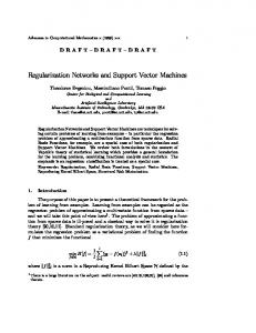
Fig. 1: Left: classification accuracy as a function of λ; right: classification accuracy of different kernels. Joint regularization is used to combine these two kernels (see Section 2.3). The classification accuracy for ten-fold cross validation as a function of λ is plotted in Figure 1(left). To test the efficacy of our method, we also tested the classification accuracy using four other kernels, namely kGauss and klinear alone, and their sum, kadd ,
459
ESANN'2005 proceedings - European Symposium on Artificial Neural Networks Bruges (Belgium), 27-29 April 2005, d-side publi., ISBN 2-930307-05-6.
and their pointwise product, kmult . We contrast their performance with that of the best joint regularization kernel in Figure 1(right). The joint regularization kernel marginally outperforms the other kernels on the dataset. Also, observe from Figure 1(left) that the performance of the joint regularization kernel depends on the value of λ. To understand this dependence, recall that when λ is close to 0 or 1 we are regularizing very heavily in the RKHS defined by one kernel while imposing very light regularization in the complementary space. Given special prior knowledge, this might be a valid strategy to adopt. In our case, both the kernels individually yield good classification accuracies and therefore require appropriate regularization in both the RKHS. This is consistent with our observation that intermediate values of λ (0.25 - 0.5) yield the best joint kernel.
4
Discussion and Outlook
In this article, we presented a principled method for combining kernels by using joint regularization, based on an extended representer theorem. Preliminary experimental results on a subset of data from the Protein Data Bank confirm that joint regularization based methods are competitive with adhoc methods, based on prior knowledge, used for combining kernels. As more and more complex models and data structures are used in bioinformatics and other areas of applied machine learning, sophisticated combination of kernels on different data types and on data from different sources is becoming an important task. Our results indicate that joint regularization allows to combine kernels into one joint kernel that promises good generalization performance. Current research is investigating the potential of joint regularization on larger datasets in bioinformatics. Future work will combine joint regularization with approaches of kernel matrix approximation.
References [1] B. Sch¨ olkopf and A. J. Smola. Learning with Kernels. MIT Press, 2002. [2] B. Sch¨ olkopf, R. Herbrich, and A. J. Smola. A generalized representer theorem. In Proceedings of the Annual Conference on Computational Learning Theory, pages 416 – 426, 2001. [3] H. M. Berman, J. Westbrook, Z. Feng, G. Gilliland, T. N. Bhat, H. Weissig, I. N. Shindyalov, and P. E. Bourne. The protein data bank. Nucleic Acids Research, 28:235–242, 2000. [4] I. Dubchak, I. Muchnik, C. Mayor, I. Dralyuk, and S. Kim. Recognition of a protein fold in the context of the SCOP classification. Proteins: Structure, Function, and Genetics, 35:401–407, 1999. [5] T. G¨ artner, P. A. Flach, and S. Wrobel. On graph kernels: Hardness results and efficient alternatives. In B. Sch¨ olkopf and M. Warmuth, editors, Sixteenth Annual Conference on Computational Learning Theory and Seventh Kernel Workshop, COLT. Springer, 2003.
460