Minimization of Detail-preserving Regularization Functional by Newton’s Method with Continuation Raymond H. Chan, Chung-Wa Ho, Chun-Yee Leung, and Mila Nikolova
Abstract— Recently, a two-phase scheme for removing saltand-pepper impulse noise has been proposed [14]. In the first phase, an adaptive median filter is used to identify pixels which are likely to be contaminated by noise (noise candidates). In the second phase, the image is restored by minimizing a specialized regularization functional that applies only to those selected noise candidates. As an extension of this work, we propose an efficient method to accomplish the second phase. The speed of our method can be double as that of the method proposed in [14] for images contaminated by 30% salt-and-pepper noise and will be faster for higher noise level. Index Terms— Impulse noise, adaptive median filter, edgepreserving regularization, Newton’s method, continuation.
I. I NTRODUCTION Impulse noise is caused by malfunctioning pixels in camera sensors, faulty memory locations in hardware, or transmission in a noisy channel. See [4] for instance. Two common types of impulse noise are the salt-and-pepper noise and the randomvalued noise. For images corrupted by salt-and-pepper noise (respectively random-valued noise), the noisy pixels can take only the maximum and the minimum values (respectively any random value) in the dynamic range. There are many works on the restoration of images corrupted by impulse noise. See, for instance, the nonlinear digital filters reviewed in [1]. The median filter was once the most popular nonlinear filter for removing impulse noise, because of its good denoising power [4] and computational efficiency [11]. However, when the noise level is over 50%, some details and edges of the original image are smeared by the filter [16]. Different remedies of the median filter have been proposed, e.g. the adaptive median filter [12], the multi-state median filter [7], or the median filter based on homogeneity information [8], [17]. These so-called “decision-based” or “switching” filters first identify possible noisy pixels and then replace them by using the median filter or its variants, while leaving all other pixels unchanged. These filters are good at detecting noise even at a high noise level. Their main drawback is that the noisy pixels are replaced by some median value in their vicinity without taking into account local features such as the possible presence of edges. Hence details and edges are not recovered satisfactorily, especially when the noise level is high. R. H. Chan , C. W. Ho, and C. Y. Leung are with the Department of Mathematics, The Chinese University of Hong Kong, Shatin, Hong Kong (email: rchan,
[email protected],
[email protected]). This work was supported by HKRGC Grant CUHK 400503 and CUHK DAG 2060257. M. Nikolova is with the Centre de Math´ematiques et de Leurs Applications, ENS de Cachan, 61 av. du Pr´esident Wilson, 94235 Cachan Cedex (email:
[email protected])
0-7803-9134-9/05/$20.00 ©2005 IEEE
For images corrupted by Gaussian noise, least-squares methods based on edge-preserving regularization functionals [3], [5], [6], [18] have been used successfully to preserve the edges and the details in the images. These methods fail in the presence of impulse noise because the noise is heavily tailed. Moreover the restoration will alter basically all pixels in the image, including those that are not corrupted by the impulse noise. Recently, non-smooth data-fidelity terms (e.g. ℓ1 ) have been used along with edge-preserving regularization to deal with impulse noise [13]. In [14], a two-stage scheme which combines the variational method proposed in [13] with the adaptive median filter [12] is proposed. More precisely, the noise candidates are first identified by the adaptive median filter, and then these noise candidates are selectively restored using an objective function with an ℓ1 data-fidelity term and an edge-preserving regularization term. Since the edges are preserved for the noise candidates, and no changes are made to the other pixels, the performance is much better than that of either one of the methods. Salt-and-pepper noise with noise ratio as high as 90% can be cleaned quite efficiently. With slight modification, the method also applies to random-valued noise with noise level as high as 50%, see [15]. In this paper, we propose an efficient method for solving the minimization problem in phase two of the algorithm proposed in [14]. The outline of this paper is as follows. In Section II, we give a brief review of the two-phase method proposed in [14]. In Section III, we modify the functional proposed in [14] so that it is more easier to be minimized without affecting the restoration performance. In Section IV, we describe our method to minimize the edge-preserving regularization functional. In Section V, we give some experimental results. In Section VI, we conclude the paper. II. R EVIEW OF THE T WO -P HASE M ETHOD In [14], a two-phase method for detecting and removing salt-and-pepper is proposed. The first phase is the detection of noise by adaptive median filter [12] while the second phase is the restoration of the noisy image by variational method [13]. See [12] or [14] for a detailed description of adaptive median filter and [13] for a detailed description of the variational method. The two-phase algorithm in [14] combines the advantages of both methods and we will give a brief description here. In the following, we let xi,j , for (i, j) ∈ A ≡ {1, . . . , M }×{1, . . . , N }, be the gray level of a true M -by-N image x at pixel location (i, j), Vi,j be the set of four closest neighbors of (i, j), not including (i, j), and [smin , smax ] be the
I-125
dynamic range of x, i.e. smin ≤ xi,j ≤ smax for all (i, j) ∈ A. Denote by y a noisy image contaminated by salt-and-pepper noise. That is smin , with probability p, yi,j = smax , with probability q, xi,j , with probability 1 − p − q,
suggests we drop it from (1). So we may only consider the functional of the following form:
Algorithm:
IV. M INIMIZATION OF THE F UNCTIONAL The first phase of the denoising algorithm can be done quite effectively by using adaptive median filter [12]. The problem remaining is to find an effective way to minimize the functional (4). Clearly, minimizing the functional Fy,α is equivalent to solving the following equation: ´ ³ ′ ′ 2 1 Gy,α (u) , ▽Fy,α (u) = Si,j = 0 (5) + Si,j
where r = p + q defines the noise level and yi,j is the gray value of y at pixel location (i, j). The restored image ˆ. is denoted by x
˜ the image obtained by 1. (Noise detection): Denote by y applying an adaptive median filter to the noisy image y. Noticing that noisy pixels take their values in the set {smin , smax }, we define the noise candidate set as N = {(i, j) ∈ A : y˜i,j 6= yi,j and yi,j ∈ {smin , smax }} . The set of all uncorrupted pixels is N c = A \ N . 2. (Restoration): Since all pixels in N c are detected as uncorrupted, we naturally keep their original values, i.e., x ˆi,j = yi,j for all (i, j) ∈ N c . Let us now consider a noise candidate, say, at (i, j) ∈ N . Each one of its neighbors (m, n) ∈ Vi,j is either a correct pixel, i.e., (m, n) ∈ N c and hence x ˆm,n = ym,n ; or is another noise candidate, i.e., (m, n) ∈ N , in which case its value must be restored. The neighborhood Vi,j of (i, j) is thus split as Vi,j = (Vi,j ∩ N c ) ∪ (Vi,j ∩ N ). In [13], noise candidates are restored by minimizing a functional of the form (1), restricted to the noise candidate set N : ¸ X · ¯ β 1 2 ¯ Fy,α N (u) = |ui,j − yi,j | + (Si,j + Si,j ) 2 (i,j)∈N
(1)
Fy,α (u) =
1 2 where Si,j , Si,j are defined as above. Let us mention that a major difference with straightforward restoration approaches such as those in [13] is that in (4), data-fitness and regularization use the same potential function ϕα . This choice comes from the analysis developed in [13].
(i,j)∈N
′
1 Si,j
(m,n)∈Vi,j ∩N
′
1 where and are respectively the derivatives of Si,j and 2 Si,j with respect to ui,j . It is well-known that to achieve better edge-preserving result, the potential function ϕα should be close to |x| while being differentiable at zero in order to avoid stair-caising effect. So for ϕα in (2), α should be close to 0 and for ϕα in (3), α should be close to 1. However, if α is set in this way, ϕ′α will have a sharp increase near the solution, meaning that Newton’s method will diverge easily. Therefore, we apply Newton’s method with continuation as described in the following subsection, see also √ [5]. For simplicity, we describe the method for ϕα (x) = α + x2 . With slight modification, the method can be applied to other edge-preserving potential functions as well.
(m,n)∈Vi,j ∩N c
X
(4)
(i,j)∈N
2 Si,j
Newton’s Method with Continuation:
where u ∈ [0, 255]M , M , #N , X 1 Si,j = 2 · ϕα (ui,j − ym,n ), 2 = Si,j
X ¡ ¢ 1 2 Si,j + Si,j
ϕα (ui,j − um,n ),
and ϕα is an edge-preserving potential function having the parameter α. Examples of such ϕα (x) are: p (2) ϕα (x) = α + x2 , α > 0, α ϕα (x) = |x| , 1 < α ≤ 2. (3)
See [2], [3], [6], [10] and [14]. III. M ODIFICATION OF THE R EGULARIZATION F UNCTIONAL It has been shown in [13] that the term |ui,j − yi,j | in (1) allows noisy pixels to be detected, but it also introduces a small bias on the restoration of corrupted pixels. In our method, the set of all noisy pixels is detected at its first phase. At the restoration phase, this term is hence no longer necessary. This
I-126
1. Initially, we set α to a very large number α1 (in our tests, we set α1 = 160, 000). Since α1 is large, the function Gy,α1 (u) is smooth. Therefore Newton’s method converges with a wide range of initial guesses. We just take the restored image by the adaptive median filter to be the initial guess. Let xα1 be the solution obtained by applying Newton’s method to (5) with α = α1 . 2. Next we solve (5) by Newton’s method for a smaller α2 (in our tests, α2 = 5, 000). For α2 , Gy,α2 (u) becomes less smooth and we need a better initial guess so that Newton’s method can converge. Here we use xα1 as initial guess, and we denote the solution to Gy,α2 (u) = 0 by xα2 . 3. We repeat this process and reduce α each time, namely the solution to Gy,αi (u) = 0 is used as initial guess for Gy,αi+1 (u) = 0 until we have finally decreased α to our desired value. From our tests, if α is reduced using the choices ÷32
÷4
÷4
÷2
160000 −→ 5000 −→ 1250 −→ 312.5 −→ ÷2
÷2
÷2
156.25 −→ 78.125 −→ 39.0625 −→ · · ·
TABLE I C OMPARISON OF DENOISING TIME IN SECONDS FOR 256 × 256 Lena. Noise Level 10% 30% 50% 70% 90%
Adaptive Median Filter 2.4 3.0 4.1 6.2 11.6
Algorithm in [14] 6.4 22.4 53.4 96.8 241.9
Our Algorithm 5.4 11.2 19.5 30.7 65.6
TABLE II C OMPARISON OF DENOISING TIME IN SECONDS FOR 512 × 512 Lena. (a)
(b)
(c)
Noise Level 10% 30% 50% 70% 90%
Adaptive Median Filter 10.9 16.7 32.7 64.5 130.5
Algorithm in [14] 29.2 94.3 259.6 446.2 1897.0
Our Algorithm 22.8 51.5 98.6 170.3 256.7
order to test the speed of the algorithms more fairly, the experiments are repeated 10 times and the average of the 10 timings is given here. We can see from the tables that our algorithm is twice faster than the algorithm proposed in [14] at 30% noise level and as the noise level becomes higher, our algorithm denoises more faster than the algorithm proposed in [14].
(d)
VI. C ONCLUSION In this paper, we propose an efficient way to minimize the regularization functional to achieve fast and excellent denoising result. The two-phase algorithm proposed in [14] gives a good method for denoising, and we improve it by our efficient algorithm. With slight modification, our proposed algorithm can apply equally well to random-valued impulse noise (cf. [15]).
(e) Fig. 1. Restoration results of different algorithms: (a) Corrupted Lena image with 70% salt-and-pepper noise (6.7 dB), (b) Adaptive Median Filter (23.3 dB), (c) Algorithm proposed in [14] (27.3 dB), (d) Our algorithm (27.2 dB), and (e) The original image Lena.
then Newton’s Method will always converge. We remark that the Jacobian matrix systems within the Newton Method is solved by the conjugate gradient method with MILU preconditioner [19]. Next we give the test results. V. S IMULATIONS As our method performs essentially the same as that in [14], we omit the details on the denoising performance of our algorithm and focus on its speed. Figure 1 shows the results of applying the adaptive median filter, the algorithm proposed in [14], and our algorithm to the image Lena of resolution 256 × 256 corrupted by 70% salt-and-pepper noise. The peak signal to noise ratio [4] is also listed there. Tables I and II show the time required for the whole denoising process for the adaptive median filter, the algorithm proposed in [14] and our algorithm on the images contaminated by salt-and-pepper noise of different noise levels. In
R EFERENCES [1] J. Astola and P. Kuosmanen, Fundamentals of Nonlinear Digital Filtering. Boca Raton, CRC, 1997. [2] M. Black and A. Rangarajan, “On the unification of line processes, outlier rejection, and robust statistics with applications to early vision,” International Journal of Computer Vision, 19 (1996), pp. 57–91. [3] C. Bouman and K. Sauer, “On discontinuity-adaptive smoothness priors in computer vision,” IEEE Transactions on Pattern Analysis and Machine Intelligence, 17 (1995), pp. 576–586. [4] A. Bovik, Handbook of Image and Video Processing, Academic Press, 2000. [5] T. F. Chan, H. M. Zhou, and R. H. Chan, “A continuation method for total variation denoising problems,” Proceedings of SPIE Symposium on Advanced Signal Processing: Algorithms, Architectures, and Implementations, ed. F. T. Luk, 2563 (1995), pp. 314–325, [6] P. Charbonnier, L. Blanc-F´eraud, G. Aubert, and M. Barlaud, “Deterministic edge-preserving regularization in computed imaging,” IEEE Transactions on Image Processing, 6 (1997), pp. 298–311. [7] T. Chen and H. R. Wu, “Space variant median filters for the restoration of impulse noise corrupted images,” IEEE Transactions on Circuits and Systems II, 48 (2001), pp. 784–789. [8] H.-L. Eng and K.-K. Ma, “Noise adaptive soft-switching median filter,” IEEE Transactions on Image Processing, 10 (2001), pp. 242–251. [9] R. C. Gonzalez and R. E. Woods, Digital Image Processing Second Edition, Prentice Hall, 2001; and Book Errata Sheet (July 31, 2003), http://www.imageprocessingbook.com/downloads/errata sheet.htm. [10] P. J. Green, “Bayesian reconstructions from emission tomography data using a modified EM algorithm,” IEEE Transactions on Medical Imaging, MI-9 (1990), pp. 84–93.
I-127
[11] T. S. Huang, G. J. Yang, and G. Y. Tang, “Fast two-dimensional median filtering algorithm,” IEEE Transactions on Acoustics, Speech, and Signal Processing, 1 (1979), pp. 13–18. [12] H. Hwang and R. A. Haddad, “Adaptive median filters: new algorithms and results,” IEEE Transactions on Image Processing, 4 (1995), pp. 499–502. [13] M. Nikolova, “A variational approach to remove outliers and impulse noise,” Journal of Mathematical Imaging and Vision, 20 (2004), pp. 99–120. [14] R. H. Chan, C. W. Ho, and M. Nikolova, “Salt-and-Pepper Noise Removal by Median-type Noise Detector and Edge-preserving Regularization,” IEEE Transactions on Image Processing, to appear. [15] R. H. Chan, C. Hu, and M. Nikolova, “An Iterative Procedure for Removing Random-Valued Impulse Noise,” IEEE Signal Proc. Letters, 11 (2004), pp. 921–924. [16] T A. Nodes and N. C. Gallagher, Jr. “The output distribution of median type filters,” IEEE Transactions on Communications, COM-32, 1984. [17] G. Pok, J.-C. Liu, and A. S. Nair, “Selective removal of impulse noise based on homogeneity level information,” IEEE Transactions on Image Processing, 12 (2003), pp. 85–92. [18] C. R. Vogel and M. E. Oman, “Fast, robust total variation-based reconstruction of noisy, blurred images,” IEEE Transactions on Image Processing, 7 (1998), pp. 813–824. [19] T. Dupont, R. P. Kendall, and H. H. Rachford JR., “An Approximate Factorization Procedure for Solving Self-adjoint Elliptic Difference Equations,” SIAM J. Numer. Anal., 5 (1968), pp. 559–573.
I-128