May 8, 2017 - siders a multi-UAV enabled wireless communication system, where .... its advantages in performance enhance
1
Joint Trajectory and Communication Design for Multi-UAV Enabled Wireless Networks
arXiv:1705.02723v1 [cs.IT] 8 May 2017
Qingqing Wu, Yong Zeng, and Rui Zhang
Abstract Unmanned aerial vehicles (UAVs) have attracted significant interest recently in assisting wireless communication due to their high maneuverability, flexible deployment, and low cost. This paper considers a multi-UAV enabled wireless communication system, where multiple UAV-mounted aerial base stations (BSs) are employed to serve a group of users on the ground. To achieve fair performance among users, we maximize the minimum throughput over all ground users in the downlink communication by optimizing the multiuser communication scheduling and association jointly with the UAVs’ trajectory and power control. The formulated problem is a mixed integer non-convex optimization problem that is challenging to solve. As such, we propose an efficient iterative algorithm for solving it by applying the block coordinate descent and successive convex optimization techniques. Specifically, the user scheduling and association, UAV trajectory, and transmit power are alternately optimized in each iteration. In particular, for the non-convex UAV trajectory and transmit power optimization problems, two approximate convex optimization problems are solved, respectively. We further show that the proposed algorithm is guaranteed to converge to at least a locally optimal solution. To speed up the algorithm convergence and achieve good throughput, a low-complexity and systematic initialization scheme is also proposed for the UAV trajectory design based on the simple circular trajectory and the circle packing scheme. Extensive simulation results are provided to demonstrate the significant throughput gains of the proposed design as compared to other benchmark schemes.
Index Terms UAV communications, throughput maximization, optimization, trajectory design, mobility control. The authors are with the Department of Electrical and Computer Engineering, National University of Singapore, email:{elewuqq, elezeng, elezhang}@nus.edu.sg. Part of this work has been submitted to IEEE GLOBECOM 2017 [1].
2
I. I NTRODUCTION Unmanned aerial vehicles (UAVs), also commonly known as drones, have attracted significant attention in the past decade for various applications, such as surveillance and monitoring, aerial imaging, cargo delivery, etc [2]. As reported in [3], the global market for commercial UAV applications, estimated at about 2 billion dollars in 2016, will skyrocket to as much as 127 billion dollars by 2020. Equipped with advanced transceivers and batteries, UAVs are gaining increasing popularity in information technology (IT) applications due to their high maneuverability and flexibility for on-demand deployment. In particular, UAVs typically have high possibility of line-of-sight (LoS) air-to-ground communication links, which is appealing to the wireless service providers. To capitalize on this growing opportunity, several leading IT companies have launched pilot projects, such as Project Aquila by Facebook [4] and Project Loon by Google [5], for providing ubiquitous internet access worldwide by leveraging the UAV/drone technology. The 3rd Generation Partnership Project (3GPP) is also looking up into the sky and studying aerial vehicles supported by Long Term Evolution (LTE) where the initial focus is on UAV [6]. In fact, with the approval of Federal Aviation Administration (FAA), Qualcomm and AT&T have optimized LTE networks for UAV communications [7], which aims to pave the way to a widescale deployment of UAVs in the upcoming fifth generation (5G) wireless networks, especially for mission-critical use cases. Meanwhile, extensive research efforts from the academia have also been devoted to employing UAVs as different types of wireless communication platforms [8], such as aerial mobile base stations (BSs) [9]–[13], mobile relays [14], [15], and flying computing cloudlets [16], [17]. In particular, employing UAVs as aerial BSs is envisioned as a promising solution to enhance the performance of the existing cellular systems. Depending on whether the UAV’s high mobility is exploited or not, two different lines of research can be identified in the literature, namely static-UAV or mobile-UAV enabled wireless networks. The research on the static-UAV enabled wireless networks mainly focuses on the UAV deployment/placement optimization [9]–[13], with the UAVs serving as aerial quasi-static BSs to support ground users in a given area from a certain altitude. As such, the altitude and the horizonal location of the UAV can be either separately or jointly optimized for different quality-of-sevice (QoS) requirements. In particular, the authors in [11] provide an analytical approach to optimize the altitude of a UAV for providing maximum coverage for ground users. In contrast, by fixing the altitude, the horizonal positions of UAVs are optimized in [12] to minimize the number of
3
required UAV BSs to cover a given set of ground users. In three-dimensional (3D) space, a drone-enabled small cell placement optimization problem is investigated in [13] to maximize the number of users that can be covered. Besides the UAV placement optimization, exploiting the UAV’s high mobility in the mobileUAV enabled wireless networks is anticipated to unlock the full potential of UAV-ground communications. With the fully controllable UAV mobility, the communication distance between the UAV and ground users can be significantly shortened by proper UAV trajectory design and user scheduling. This is analogous and yet in sharp contrast to the existing small-cell technology [18], where the cell radius is reduced by increasing the number of small-cell BSs deployed, but at the cost of increased infrastructure expenditure. Motivated by this, the UAV trajectory design is rigorously studied in [15] and [19] for a mobile relaying system and point-to-point energyefficient system, respectively, where sequential convex optimization techniques are applied to solve the non-convex trajectory optimization problems therein. Though providing a general framework for trajectory optimization in two-dimensional (2D) space, the studies in [15] and [19] only focus on the setup with single UAV and single ground user. On the other hand, for UAV-enabled multi-user system, a novel cyclical multiple access scheme is proposed in [20], where the UAV communicates with ground users when it flies sufficiently close to each of them in a periodic (cyclical) time-division manner. An interesting throughput-access delay tradeoff is revealed and it has been shown that significant throughput gains can be achieved over the case of a static UAV for delay-tolerant applications. However, only one single UAV with the constant flying speed is considered in [20], and the ground users are assumed to be uniformly located in a one-dimensional (1D) line, which simplifies the analysis but limits the applicability in practice. In this paper, we study a general multi-UAV enabled wireless communication system, where multiple UAVs are employed to serve a group of users on the ground in a given 2D area. Although a single UAV has demonstrated its advantages in performance enhancement for wireless networks [15], [19], it has limited capability in general and may not guarantee availability during the entire mission due to its practical size, weight and power (SWAP) constraints [8]. This thus motivates the deployment of multiple or a swarm of UAVs which cooperatively serve the ground users to achieve more efficient communications. For example, a group of UAVs may be deployed to keep track of the participants in a large-area event and to form a multi-hop communication network connecting to the ground audience. More importantly, in a multi-UAV enabled network, users could be served in parallel with higher throughput and lower access delay, which could effectively
4
alleviate the fundamental throughput-access delay tradeoff in single-UAV communications [20]. Without loss of generality, we consider that all UAVs share the same frequency band for their communications with the ground users. By focusing on the downlink transmission from the UAVs to ground users, our goal is to maximize the minimum average rate among all users by jointly optimizing the user communication scheduling and association, and the UAV trajectory and transmit power control in a given finite period. Such a joint optimization problem is practically appealing, but has not been investigated in the literature to the authors’ best knowledge. On one hand, by properly designing the trajectories of different UAVs, not only short-distance LoS links can be proactively and dynamically established for those desired UAV-user pairs, but also the interfering channel distances between the undesired UAV-user pairs can be enlarged to alleviate the co-channel interference. On the other hand, in the occasional scenarios when the UAVs have to get close with each other for serving nearby users, their transmission power can be adjusted to reduce interference. While maximum transmission power is used for maximizing spectrum efficiency when the UAVs are far apart to serve users that are well separated. Therefore, the system performance can benefit from different design dimensions of the proposed joint optimization. However, such a joint trajectory and adaptive communication design problem is non-trivial to solve. This is because the user scheduling and association, UAV trajectory optimization, and transmit power control are closely coupled with each other in our considered problem, which makes it challenging to solve in general. To tackle the above challenges, we first relax the binary variables for user scheduling and association into continuous variables and solve the resulting problem with an efficient iterative algorithm by leveraging the block coordinate descent method [21]. Specifically, the entire optimization variables are partitioned into three blocks for the user scheduling and association, UAV trajectory, and transmit power control, respectively. Then, these three blocks of variables are alternately optimized in each iteration, i.e., one block is optimized at each time while keeping the other two blocks fixed. However, even with fixed user scheduling and association, the UAV trajectory optimization problem with fixed power control and the UAV power control problem with fixed trajectory are still difficult to solve due to their non-convexity. We thus apply the successive convex optimization technique to solve them approximately. We show that our proposed algorithm is guaranteed to converge to at least a locally optimal solution of the joint optimization problem. To speed up the algorithm convergence and achieve a superior performance, we propose an efficient and systematic trajectory initialization scheme based on the
5
Information Signal Interference
Fig. 1. A multi-UAV enabled wireless network.
simple circular trajectory and the circle packing scheme. Numerical results show that significant throughput gains are achieved by our proposed joint design, as compared to conventional static UAV or other benchmark schemes with heuristic UAV trajectories. It is also shown that the throughput of the proposed mobile UAV system increases with the UAV trajectory design period, revealing the general throughput-access delay tradeoff [1], [20] in multi-UAV enabled communications. In addition, compared to the single-UAV case, this tradeoff is shown to be significantly improved by the use of multiple UAVs. The rest of this paper is organized as follows. Section II introduces the system model and the problem formulation for a multi-UAV enabled wireless network. In Section III, we propose an efficient iterative algorithm by applying the block coordinate descent and the successive convex optimization techniques. Section VI presents the numerical results to demonstrate the performance of the proposed design. Finally, we conclude the paper in Section VI. Notations: In this paper, scalars are denoted by italic letters, vectors and matrices are respectively denoted by bold-face lower-case and upper-case letters. RM ×1 denotes the space of M-dimensional real-valued vector. For a vector a, kak represents its Euclidean norm and aT ˙ denotes its transpose. For a time-dependent function x(t), x(t) denotes the derivative with respect to time t. For a set K, |K| denotes its cardinality.
6
II. S YSTEM M ODEL
AND
P ROBLEM F ORMULATION
A. System Model As shown in Fig. 1, we consider a wireless communication system where M ≥ 1 UAVs are employed to serve a group of K > 1 ground users. The user and UAV sets are denoted as K and M, respectively, where |K| = K and |M| = M. We study the downlink communication scenario from the UAVs to ground users while the problem formulation and the results are extendible to the uplink communication scenario from ground users to the UAVs as well. This practically corresponds to an information broadcast system (in the downlink) or a data collection system (in the uplink) enabled by UAVs. Assume that all the UAVs share the same frequency band for communication over consecutive periods each of duration T > 0 in second (s). During any period, each of the UAVs serves its associated ground users via a periodic/cyclical time-division multiple access (TDMA). Note that the choice of T has a significant impact on the system performance. On one hand, thanks to the UAV mobility, a larger period T provides more time for each UAV to move closer to its served users to achieve better communication channels, as well as to fly sufficiently away from the users served by other UAVs for more effective interference mitigation, thus achieving a higher throughput. On the other hand, however, a larger T in general implies a larger access delay for users since each user may need to wait for a longer time to communicate with a UAV from one period to another. Therefore, the period T needs to be properly chosen in practice to strike a balance between the user throughput and access delay, i.e., there exists a fundamental throughput-access delay tradeoff [20] in UAV-enabled communications. Without loss of generality, we consider a 3D Cartesian coordinate system where the horizon coordinate of each ground user i is fixed at wi = [xi , yi ]T ∈ R2×1 , i ∈ K. All UAVs are assumed to fly at a fixed altitude H above ground and the time-varying horizonal coordinate of UAV m ∈ M at time instant t is denoted by qm (t) = [xm (t), ym (t)]T ∈ R2×1 , with 0 ≤ t ≤ T . The UAV trajectories need to satisfy the following constraint qm (0) = qm (T ), ∀ m,
(1)
which implies that each UAV needs to return to its initial location by the end of each period T such that users can be served periodically in the next period. In practice, the trajectories of
7
UAVs are also subject to the maximum speed constraints1, i.e, ||q˙ m (t)|| ≤ Vmax , 0 ≤ t ≤ T, ∀ m,
(2)
where Vmax denotes the maximum UAV speed in meter/second (m/s). For ease of exposition, the period T is discretized into N equal-time slots, indexed by n = 1, ..., N. The elemental slot length δt =
T N
is chosen to be sufficiently small such that a UAV’s location is considered
as approximately unchanged within each time slot even at the maximum speed Vmax . As a result, the trajectory of UAV m can be approximated by the N two-dimensional sequences qm [n] = [xm [n], ym [n]]T , n = 1, · · · , N. Furthermore, the trajectory constraints (1) and (2) can be equivalently written as qm [1] = qm [N],
(3)
2 ||qm [n + 1] − qm [n]||2 ≤ Smax , n = 1, ..., N − 1,
(4)
where Smax , Vmax δt is the maximum horizonal distance that the UAV can travel in each time slot. In fact, any required accuracy of the adopted discrete-time approximation can be always satisfied by choosing a minimum N, as follows. To guarantee a certain accuracy, the ratio of Smax and H can be restricted below a threshold, i.e.,
Smax H
≤ εmax , where εmax is the given
threshold. Then, the minimum number of time slots required for achieving the accuracy with a given εmax can be obtained as N≥
Vmax T . Hεmax
(5)
However, further increasing N also increases our design complexity. Therefore, the number of time slots N can be properly chosen in practice to balance between the accuracy and complexity. The distance from UAV m to user i in time slot n can be expressed as p di,m [n] = H 2 + ||qm [n] − wi ||2 .
(6)
For simplicity, we assume that the communication links from the UAV to the ground users are dominated by the LoS links where the channel quality depends only on the UAV-user distance. Furthermore, the Doppler effect caused by the UAV mobility is assumed to be well compensated 1
Here, we do not consider the minimum speed constraints, which is practically valid for the rotary-wing UAVs with the
capability of keeping stationary at fixed positions, i.e., a minimum zero-speed is feasible. However, for the fixed-wing UAVs that must move forward to remain aloft, additional minimum speed constraints, i.e., ||q˙ m (t)|| ≥ Vmin > 0, 0 ≤ t ≤ T, ∀ m, need to be imposed [19], which can be handled by the proposed algorithm with only a minor modification.
8
at the receivers. Thus, the channel power gain from UAV m to user i during slot n follows the free-space path loss model, which can be expressed as hi,m [n] = ρ0 d−2 i,m [n] =
H2
ρ0 , + ||qm [n] − wi ||2
(7)
where ρ0 denotes the channel power at the reference distance d0 = 1 m. Define a binary variable αi,m [n], which indicates that user i is served by UAV m in time slot n if αi,m [n] = 1; otherwise, αi,m [n] = 0. As such, αi,m [n] specifies not only the user communication scheduling across the different time slots, but also the UAV-user association for each time slot. We assume that in each time slot, each UAV only serves at most one user and each user is only served by at most one UAV, which yields the following constraints K X
αi,m [n] ≤ 1, ∀ m, n,
(8)
αi,m [n] ≤ 1, ∀ i, n,
(9)
i=1
M X
m=1
αi,m [n] ∈ {0, 1}, ∀ i, m, n.
(10)
The downlink transmit power of UAV m, m ∈ M in time slot n is denoted by pm [n], which is subject to the constraint 0 ≤ pm [n] ≤ Pmax , with Pmax denoting the peak UAV transmission power. Thus, if user i is served by UAV m in time slot n, i.e., αi,m [n] = 1, the corresponding received signal-to-interference-plus-noise ratio (SINR) at user i can be expressed as γi,m [n] = PM
pm [n]hi,m [n]
2 j=1,j6=m pj [n]hi,j [n] + σ
,
(11)
where σ 2 is the power of the additive white Gaussian noise (AWGN) at the receiver. The term PM j=1,j6=m pj [n]hi,j [n] in the denominator of (11) represents the co-channel interference caused
by the transmissions of all other UAVs in time slot n. Thus, the achievable rate of user i in time slot n, denoted by Ri [n] in bits/second/Hertz (bps/Hz), can be expressed as Ri [n] =
M X
αi,m [n] log2 (1 + γi,m [n]) .
(12)
m=1
Thus, the achievable average rate of user i over N time slots is given by pm [n]ρ0 N N X M X X 1 1 H 2 +||qm [n]−wi ||2 Ri [n] = αi,m [n] log2 1 + PM Ri = pj [n]ρ0 N n=1 N n=1 m=1 2
j=1,j6=m H +||qj [n]−wi ||2
+
σ2
.
(13)
9
B. Problem Formulation Let A = {αi,m [n], ∀ i, m, n}, Q = {qm [n], ∀ m, n}, and P = {pm [n], ∀ m, n}. By assuming that the locations of the ground users are known, our goal is to maximize the minimum average rate among all users by jointly optimizing the user scheduling and association (i.e., A), UAV trajectory (i.e., Q), and transmit power (i.e., P) over all time slots. Define η(A, Q, P) = min Ri i∈K
as a function of A, Q, and P. The optimization problem is formulated as max
A,Q,P
s.t.
η
(14a)
N M 1 XX αi,m [n] log2 (1 + γi,m [n]) ≥ η, ∀ i, N n=1 m=1
K X
(14b)
αi,m [n] ≤ 1, ∀ m, n,
(14c)
αi,m [n] ≤ 1, ∀ i, n,
(14d)
i=1
M X
m=1
αi,m [n] ∈ {0, 1}, ∀ i, m, n,
(14e)
2 ||qm [n + 1] − qm [n]||2 ≤ Smax , n = 1, ..., N − 1,
(14f)
qm [1] = qm [N], ∀ m,
(14g)
0 ≤ pm [n] ≤ Pmax , ∀ m, n.
(14h)
Problem (14) is challenging to solve due to the following two main reasons. First, the optimization variables A for user scheduling and association are binary and thus (14c)-(14e) involve integer constraints. Second, even with fixed user scheduling and association, (14b) is still a non-convex constraint with respect to UAV trajectory variables Q and/or transmit power variables P. Therefore, problem (14) is a mixed-integer non-convex problem, which is difficult to be optimally solved in general. Before proceeding to solve problem (14), we first discuss two special cases for for interference-free scenarios. C. Special Case I: A Single UAV First, when only one UAV is deployed to serve all the ground users, i.e., M = 1, there is no co-channel interference in the system [1]. For ease of exposition, we drop the UAV index and
10
let α = {αi [n], ∀ n}. Thus, the average achievable rate of user i in (13) reduces to � � N p[n]ρ0 1 X I αi [n] log2 1 + . Ri = N n=1 (H 2 + ||q[n] − wi ||2 )σ 2
(15)
It is not difficult to see that, the UAV should always transmit with its maximum power, i.e., p[n] = Pmax , ∀ n. In this case, problem (14) is simplified to a joint user scheduling and UAV trajectory optimization problem, i.e., max α,Q
s.t.
min RiI
(16a)
i∈K
K X
αi [n] ≤ 1, ∀ n,
(16b)
i=1
αi [n] ∈ {0, 1}, ∀ i, n,
(16c)
2 ||q[n + 1] − q[n]||2 ≤ Smax , n = 1, ..., N − 1,
(16d)
q[1] = q[N].
(16e)
Since problem (16) is a special case of problem (14), the optimization framework proposed in Section III is also applicable to problem (16). D. Special Case II: Orthogonal UAV Transmission For the second special case, the multiple UAVs take turns to transmit information to their served ground users over orthogonal time slots, thus the system is also interference-free. This is achieved by imposing the following constraints2, K X
αi,m [M(ℓ − 1) + m] ≤ 1, ∀ m, ℓ = 1, 2, · · ·,
i=1
K X
N , M
αi,j [M(ℓ − 1) + m] = 0, ∀ j 6= m, ℓ = 1, 2, · · ·,
i=1
(17) N , M
(18)
which guarantee that in each time slot, only one UAV is allowed to transmit. Accordingly, the achievable rate of user i can be expressed as RiII
2
� � N M pm [n]ρ0 1 XX αi,m [n] log2 1 + . = N n=1 m=1 (H 2 + ||qm [n] − wi ||2 )σ 2
For convenience, we select the value of N such that
N M
is an integer for a given M .
(19)
11
Therefore, problem (14) can be reformulated as max
A,Q,P
s.t.
RiII
(20a)
(17), (18),
(20b)
(14e), (14f), (14g), (14h).
(20c)
min i∈K
Note that problem (20) is obtained from problem (14) by replacing the constraints (14c) and (14d) with (20b). It can be shown that (20b) and (14e) implies (14c) and (14d), but not vice versa. Thus, problem (20) is regarded as a special case of problem (14), and thus can be solved similarly as shown in the next section. III. P ROPOSED A LGORITHM To make problem (14) more tractable, we first relax the binary variables in (14e) into continuous variables, which yields the following problem max
A,Q,P
η
s.t. 0 ≤ αi,m [n] ≤ 1, ∀ i, m, n, (14b), (14c), (14d), (14f), (14g), (14h).
(21a) (21b) (21c)
Such a relaxation in general implies that the objective value of problem (21) serves as an upper bound for that of problem (14). Although relaxed, problem (21) is still a non-convex optimization problem due to the non-convex constraint (14b). In general, there is no standard method for solving such non-convex optimization problems efficiently. In the following, we propose an efficient iterative algorithm for the relaxed problem (21) by applying the block coordinate descent and successive convex optimization techniques [21]. Specifically, for given UAV trajectory Q and transmit power P, we optimize the user scheduling and association A by solving a linear programming (LP). For any given user scheduling and association A and transmit power P (UAV trajectory Q), the UAV trajectory Q (transmit power P) is optimized based on the successive convex optimization technique. Then, we present the overall algorithm and analytically show its convergence. Furthermore, we propose a low-complexity initialization scheme for the UAV trajectory design. Finally, we show how to reconstruct a binary solution to the original problem (14) based on the obtained solution to problem (21).
12
A. User Scheduling and Association Optimization For any given UAV trajectory and transmit power {Q, P}, the user scheduling and association of problem (21) can be optimized by solving the following problem η
max η,A
s.t.
(22a)
N M 1 XX αi,m [n] log2 (1 + γi,m [n]) ≥ η, ∀ i, N n=1 m=1
K X
(22b)
αi,m [n] ≤ 1, ∀ m, n,
(22c)
αi,m [n] ≤ 1, ∀ i, n,
(22d)
i=1
M X
m=1
0 ≤ αi,m [n] ≤ 1, ∀ i, m, n.
(22e)
Since problem (22) is a standard LP, it can be solved efficiently by existing optimization tools such as CVX [22]. Furthermore, it is easy to see that the constraints (22c) and (22d) are met with equalities when the optimal solution A is attained for given {Q, P}. B. UAV Trajectory Optimization For any given user scheduling and association as well as UAV transmit power {A, P}, the UAV trajectory of problem (21) can be optimized by solving the following problem max η,Q
η
(23a)
M N X X 1 αi,m [n] log2 1 + PM s.t. N n=1 m=1
pm [n]ρ0 H 2 +||qm [n]−wi ||2 pj [n]ρ0 j=1,j6=m H 2 +||qj [n]−wi ||2
2 ||qm [n + 1] − qm [n]||2 ≤ Smax , n = 1, ..., N − 1,
qm [1] = qm [N], ∀ m.
+
σ2
≥ η, ∀ i,
(23b) (23c) (23d)
Note that problem (23) is neither a concave or quasi-concave maximization problem due to the non-convex constraints in (23b). In general, there is no efficient method to obtain the
13
optimal solution. In the following, we adopt the successive convex optimization technique for the trajectory optimization. To this end, Ri,m [n], in constraints (23b) can be written as pm [n]ρ0 H 2 +||qm [n]−wi ||2 pj [n]ρ0 j=1,j6=m H 2 +||qj [n]−wi ||2
Ri,m [n] = log2 1 + PM
M X
+ σ2
pj [n]ρ0 + σ2 2 2 H + ||q [n] − w || j i j=1,j6=m
ˆ i,m [n] − log2 =R
!
,
(24)
where ˆ i,m [n] = log2 R
M X j=1
pj [n]ρ0 + σ2 2 H + ||qj [n] − wi ||2
!
.
(25)
With (24) and (25), constraints (23b) are transformed into N M 1 XX ˆ i,m [n] − log2 αi,m [n] R N n=1 m=1
M X
pj [n]ρ0 + σ2 2 2 H + ||q j [n] − wi || j=1,j6=m
!!
≥ η, ∀ i.
(26)
Note that constraints in (26) are still non-convex. By introducing slack variables S = {Si,j [n] = ||qj [n] − wi ||2 , ∀ j 6= m, j ∈ M, i, n}, problem (23) can be reformulated as max
η,Q,S
s.t.
η N M 1 XX ˆ i,m [n] − log2 αi,m [n] R N n=1 m=1
(27a) M X
pj [n]ρ0 + σ2 2 H + S [n] i,j j=1,j6=m
!!
≥ η, ∀ i,
(27b)
Si,j [n] ≤ ||qj [n] − wi ||2 , ∀ i, j 6= m, n,
(27c)
2 ||qm [n + 1] − qm [n]||2 ≤ Smax , n = 1, ..., N − 1,
(27d)
qm [1] = qm [N], ∀ m.
(27e)
It can be verified that without loss of optimality to problem (27), all constraints in (27c) can be met with equality, since otherwise we can always increase Si,j [n] without decreasing the ˆ i,m [n] is neither convex nor concave with respect to qj [n]. objective value. Note that in (27b), R While in (27c), even though ||qj [n] − wi ||2 is convex with respect to qj [n], the resulting set is not a convex set since the superlevel set of a convex quadratic function is not convex in general. Thus, problem (27) is still a non-convex optimization problem due to the non-convex feasible set. To tackle the non-convexity of (27b) and (27c), the successive convex optimization technique can be applied where in each iteration, the original function is approximated by a more tractable
14
function at a given local point. Specifically, define Qr = {qrm [n], ∀ m, n} as the given trajectory ˆ i,m [n] is not concave of UAVs in the r-th iteration. The key observation is that in (25), although R with respect to qj [n], it is convex with respect to ||qj [n] − wi ||2 . Recall that any convex function is globally lower-bounded by its first-order Taylor expansion at any point [23]. Therefore, with ˆ i,m [n], i.e., given local point Qr in the r-th iteration, we obtain the following lower bound for R
ˆ i,m [n] = log2 R
M X j=1
≥
M X j=1
pj [n]ρ0 + σ2 2 H + ||qj [n] − wi ||2
!
� r −Ari,j [n] ||qj [n] − wi ||2 − ||qrj [n] − wi ||2 + Bi,j [n]
lb ˆ i,m ,R [n],
(28)
r where Ari,j [n] and Bi,j [n] are constants that are given by
Ari,j [n]
pj [n]ρ0 (H 2 +||qrj [n]−wi ||2 )2
= PM
l=1
r Bi,j [n] = log2
log2 (e)
pl [n]ρ0 H 2 +||qrl [n]−wi ||2 M X l=1
+ σ2
, ∀ i, j, n,
pl [n]ρ0 + σ2 r 2 2 H + ||ql [n] − wi ||
(29) !
, ∀ i, j, n.
(30)
Similarly, in constraints (27c), since ||qj [n] − wi ||2 is a convex function with respect to qj [n], we have the following inequality by applying the first-order Taylor expansion at the given point qrj [n], ||qj [n] − wi ||2 ≥ ||qrj [n] − wi ||2 + 2(qrj [n] − wi )T (qj [n] − qrj [n]), ∀ i, j 6= m, n.
(31)
With any given local point Qr as well as the lower bounds in (28) and (31), problem (27) is approximated as the following problem max
r ,Q,S ηtrj
s.t.
r ηtrj N M 1 XX ˆ lb [n] − log2 αi,m [n] R i,m N n=1 m=1
(32a) M X
pj [n]ρ0 + σ2 2 H + S i,j [n] j=1,j6=m
!!
r ≥ ηtrj , ∀ i,
(32b)
Si,j [n] ≤ ||qrj [n] − wi ||2 + 2(qrj [n] − wi )T (qj [n] − qrj [n]), ∀ i, j 6= m, n,
(32c)
2 ||qm [n + 1] − qm [n]||2 ≤ Smax , n = 1, ..., N − 1,
(32d)
qm [1] = qm [N], ∀ m.
(32e)
15
Since the left-hand-side (LHS) of the constraint (32b) is jointly concave with respect to qrj [n] and Si,j [n], it is convex now. Furthermore, both (32c) and (32d) are convex quadratic constraints and (32e) is a linear constraint. Therefore, problem (32) is a convex optimization problem that can be efficiently solved by standard convex optimization solvers such as CVX [23]. It is worth noting that the lower bounds adopted in (32b) and (32c) suggest that any feasible solution of problem (32) is also feasible for problem (27), but the reverse does not hold in general. As a result, the optimal objective value obtained from the approximate problem (32) in general serves as a lower bound of that of problem (27). C. UAV Transmit Power Control For any given user scheduling and association as well as UAV trajectory {A, Q}, the UAV transmit power of problem (21) can be optimized by solving the following problem max η,P
s.t.
η
(33a)
N M 1 XX αi,m [n] log2 N n=1 m=1
1 + PM
pm [n]hi,m [n]
j=1,j6=m pj [n]hi,j [n]
+ σ2
!
0 ≤ pm [n] ≤ Pmax , ∀ m, n.
≥ η, ∀ i,
(33b) (33c)
Problem (33) is a non-convex optimization problem due to the non-convex constraint (33b). Note that the LHS of (33b), i.e., Ri,m [n], can be written as a difference of two concave functions with respect to the power control variables, i.e., Ri,m [n] = log2 = log2
1 + PM
pm [n]hi,m [n]
j=1,j6=m pj [n]hi,j [n]
M X
pj [n]hi,j [n] + σ 2
j=1
!
+ σ2
!
ˇ i,m [n], −R
(34)
!
(35)
where ˇ i,m [n] = log2 R
M X
j=1,j6=m
pj [n]hi,j [n] + σ 2
.
To handle the non-convex contraint of (33b), we apply the successive convex optimization ˇ i,m [n] with a convex function in each iteration. Specifically, define technique to approximate R Pr = {prm [n], ∀ m, n} as the given transmit power of UAV m in the r-th iteration. Recall that
16
any concave function is globally upper-bounded by its first-order Taylor expansion at any point [23]. Thus, we have the following convex upper bound at the given local point prj [n], ! M X ˇ i,m [n] = log2 pj [n]hi,j [n] + σ 2 R j=1,j6=m
≤
M X
j=1,j6=m
� Di,j [n] pj [n] − prj [n] + log2
M X
prj [n]hi,j [n] + σ 2
j=1,j6=m
!
ub ˇ i,m ,R [n],
(36)
where Di,j [n] = PM
hi,j [n] log2 (e)
l=1,l6=m
prj [n]hi,l [n] + σ 2
, ∀ i, j, n.
(37)
ˇ ub [n] in (36), problem (33) is approxWith any given local point Pr and the upper bound R i,m imated as the following problem r max ηpow
(38a)
r ηpow ,P
N M 1 XX αi,m [n] log2 s.t. N n=1 m=1
M X
pj [n]hi,j [n] + σ 2
j=1
0 ≤ pm [n] ≤ Pmax , ∀ m, n.
!
ˇ ub [n] −R i,m
!
r ≥ ηpow , ∀ i,
(38b) (38c)
Problem (38) is a convex optimization problem, which can be efficiently solved by standard convex optimization solvers such as CVX [23]. It is also worth noting that the upper bound adopted in (38b) suggests that the feasible set of problem (38) is always a subset of that of problem (33). Therefore, the optimal objective value obtained from problem (38) in general serves as a lower bound of that of problem (33). D. Overall Algorithm and Convergence Based on the results presented in the previous three subsections, we propose an overall iterative algorithm for problem (21) by applying the block coordinate descent method [24], also known as the alternating optimization method. Specifically, the entire optimization variables in original problem (21) are partitioned into three blocks, i.e., {A, Q, P}. Then, the user scheduling and association A, UAV trajectory Q, and transmit power P are alternately optimized, by solving problem (22), (32), and (38) correspondingly, while keeping the other two blocks of variables fixed. Furthermore, the obtained solution in each iteration is used as the input of the next
17
Algorithm 1 Block coordinate descent algorithm for problem (21). 1: Initialize Q0 and P0 . Let r = 0. 2:
repeat
3:
Solve problem (22) for given {Qr , Pr }, and denote the optimal solution as {Ar+1 }.
4:
Solve problem (32) for given {Ar+1 , Qr , Pr }, and denote the optimal solution as {Qr+1 }.
5:
Solve problem (38) for given {Ar+1, Qr+1 , Pr }, and denote the optimal solution as {Pr+1}.
6: 7:
Update r = r + 1. until The fractional increase of the objective value is below a threshold ǫ > 0.
iteration. The details of this algorithm are summarized in Algorithm 1. It is worth pointing out that in the classical block coordinate descent method, the sub-problem for updating each block of variables is required to be solved exactly with optimality in each iteration in order to guarantee the convergence [24]. However, in our case, for the trajectory optimization problem (23) and transmit power optimization problem (33), we only solve their approximate problems (32) and (38) optimally. Thus, the convergence analysis for the classical coordinate descent method cannot be directly applied and the convergence of Algorithm 1 needs to be proved, as shown next. lb,r r lb,r r r r where ηtrj and ηpow are respectively (A, Q, P) = ηpow Define ηtrj (A, Q, P) = ηtrj and ηpow
the objective values of problem (32) and (38) based on A, Q, and P. First, in step 3 of Algorithm 1, since the optimal solution of (22) is obtained for given Qr and Pr , we have η(Ar , Qr , Pr ) ≤ η(Ar+1, Qr , Pr ),
(39)
where η(A, Q, P) is defined prior to problem (14). Second, for given Ar+1, Qr , and Pr in step 4 of Algorithm 1, it follows that (a)
(b)
lb,r lb,r η(Ar+1, Qr , Pr ) = ηtrj (Ar+1 , Qr , Pr ) ≤ ηtrj (Ar+1 , Qr+1 , Pr ) (c)
≤ η(Ar+1, Qr+1 , Pr ),
(40)
where (a) holds since the first-order Taylor expansions in (28) and (31) are tight at the given local points, respectively, which means that problem (32) at Qr has the same objective value as that of problem (23); (b) holds since in step 4 of Algorithm 1 with the given Ar+1 and Pr , problem (32) is solved optimally with solution Qr+1 ; (c) holds since the objective value of problem (32)
18
is the lower bound of that of its original problem (23) at Qr+1 . The inequality in (40) suggests that although only an approximate optimization problem (32) is solved for obtaining the UAV trajectory, the objective value of problem (23) is still non-decreasing after each iteration. Third, for given Ar+1 , Qr+1 , and Pr in step 5 of Algorithm 1, it follows that (d)
(e)
lb,r lb,r η(Ar+1 , Qr+1 , Pr ) = ηpow (Ar+1 , Qr+1 , Pr ) ≤ ηpow (Ar+1, Qr+1 , Pr+1 ) (f )
≤ η(Ar+1 , Qr+1 , Pr+1),
(41)
where (d) holds since the first-order Taylor expansion in (36) is tight at the given local point which means that problem (38) at Pr has the same objective value as that of problem (33); (b) holds since in step 5 of Algorithm 1 with the given Ar+1 and Qr+1 , problem (32) is solved optimally with solution Pr+1 ; (c) holds since the objective value of problem (32) is the lower bound of that of its original problem (23) at Pr+1 . Based on (39)–(41), we obtain η(Ar , Qr , Pr ) ≤ η(Ar+1, Qr+1 , Pr+1),
(42)
which indicates that the objective value of problem (21) is non-decreasing after each iteration of Algorithm 1. Since the objective value of problem (21) is upper bounded by a finite value, the proposed Algorithm 1 is guaranteed to converge. Furthermore, it can be verified that all the lower bound and upper bound functions adopted in (28), (31), and (36) have the same gradients as their original functions at the given local points, respectively. Thus, Algorithm 1 is guaranteed to converge to at least a locally optimal solution based on the recent results in [21]. Note that in Algorithm 1, the UAV trajectory has to be initialized. It is known that for locally optimal algorithms, the converged solution and the ultimate system performance in general depend on the initialization schemes. Thus, we further propose an efficient trajectory initialization scheme, which is elaborated in the next subsection. E. Trajectory Initialization Scheme In this subsection, we propose a low-complexity and systematic initialization scheme for the trajectory design in Algorithm 1 based on the simple circular trajectory and the circle packing scheme. Specifically, the initial trajectory of each UAV is set to be a circular trajectory with the UAV speed taking a constant value V , with 0 < V ≤ Vmax . Furthermore, the radius of the initial trajectory circles are assumed to be the same for all UAVs. The center and radius of the circular m m T trajectories are denoted by cm trj = [xtrj , ytrj ] and rtrj , respectively. Thus, for any given period T ,
19
Fig. 2. An example of UAV trajectories initialization based on circle packing for M = 2 (left) and M = 3 (right). The black dots and the dashed blue circles are the results obtained from the circle packing scheme. The solid red circles are the initial circular trajectories of UAVs.
we have 2πrtrj = V T . Intuitively, circles that correspond to the initial trajectories of different UAVs should be sufficiently separated to minimize the co-channel interference, and at the same time, all circles together should cover the entire area as much as possible so as to better balance the users’ rates. Therefore, the initial circular trajectories are obtained based on circle packing. To this end, we first determine the geometric center of users as cg =
PK
i=1
wi
K
. The radius of the
minimum circle with cg as the circle center which can cover all users is denoted by ru , which is equal to the maximum distance between cg and all the users, i.e., ru = max ||wi −cg ||. Given the i∈K
number of UAVs M and ru , we exploit the circle packing (CP) scheme [25], also known as point packing, to obtain the center of each of the M circles cm trj as well as the corresponding radius r cp . To balance the number of users inside and outside the circular trajectory,
r cp 2
is a reasonable
choice for the trajectory circle radius. However, due to the maximum UAV speed constraint, the resulting radius
r cp 2
may not be always achievable given the finite time T if πr cp > Vmax T . In
this case, the maximum allowed radius is computed as rmax =
Vmax T . 2π
(43)
As such, the radius of the initial circular trajectory is set as rtrj = min(rmax , r2cp ). Let θn , , ∀ n, and Q0 = {q0m [n], ∀ m, n}. Based on cm 2π (n−1) trj and rtrj , the initial trajectory of UAV m N −1 in time slot n is then obtained as � �T m q0m [n] = xm + r cos θ , y + r sin θ , n = 1, ..., N. trj n trj n trj trj
(44)
20
F. Reconstruct the Binary User Scheduling and Association Solution Note that Algorithm 1 is to solve the relaxed problem (21) where the binary user scheduling and association variables in the original problem (14) are relaxed to continuous variables between 0 and 1. Thus, in the solution obtained by Algorithm 1, if the user scheduling and association variables αi,m [n] are all binary, then the relaxation is tight and the obtained solution is also a locally optimal solution of problem (14). Otherwise, the binary user scheduling and association solution needs to be reconstructed based on the solution obtained for (21). To this end, we further divide each time slot into τ sub-slots so that the new total number of sub-slots is N ′ = τ N, τ ≥ 1. Then, the number of sub-slots assigned to user i by UAV m in time slot n is Ni,m [n] = ⌊τ αi,m [n]⌉, where ⌊x⌉ denotes the nearest integer of x. It is not difficult to see that as τ increases, Ni,m [n] approaches an integer which allows a binary solution. For example, consider a single-UAV enabled two-user system with α1 [ℓ] = 0.69 and α2 [ℓ] = 0.31 in time slot ℓ, where the UAV index is dropped for convenience. If τ = 1, we have N1 [ℓ] = ⌊0.69] = 1 and N2 [ℓ] = ⌊0.31⌉ = 0, respectively. If each time slot is further divided into 10 sub-slots, i.e., τ = 10, then N1 [ℓ] = ⌊6.9⌉ = 7 and N2 [ℓ] = ⌊3.1⌉ = 3, respectively. Although such a rounding still causes a performance gap, the gap decreases as the duration of the sub-slot decreases. Alternatively, if each time slot is divided into 100 sub-slots, i.e., τ = 100, user 1 and user 2 will be assigned 69 and 31 sub-slots, respectively, i.e., N1 [ℓ] = ⌊69⌉ = 69 and N2 [ℓ] = ⌊31⌉ = 31, which permits a binary solution with zero relaxation gap. Furthermore, since constraints (22c) and (22d) are met with equalities in the optimal solution to problem (22), a binary solution for the case of multiple UAVs can be easily reconstructed by applying the above procedure. IV. N UMERICAL R ESULTS In this section, we provide numerical examples to demonstrate the effectiveness of the proposed algorithm. We consider a system with K = 6 ground users that are randomly and uniformly distributed within a 2D area of 2 × 2 km2. The following results are obtained based on one random realization of the user locations as shown in Fig. 3. All the UAVs are assumed to fly at a fixed altitude H = 100 m. The receiver noise power is assumed to be σ 2 = −110 dBm. The channel power gain at the reference distance d0 = 1 m is set as ρ0 = −60 dB. The maximum transmit power and the maximum speed of UAVs are assumed as Pmax = 0.1 W and Vmax = 50 m/s, respectively. The threshold ǫ in Algorithm 1 is set as 10−4 . The transmit power of the UAVs is initialized by the maximum transmit power, i.e., pm [n] = Pmax , ∀ m.
21
1200 T = 30 s T = 60 s T = 210 s
1000 800
t = 35 s t = 70 s
600
y(m)
400
t = 105 s
t=0s
200 0 −200 −400 −600
t = 175 s
t = 140 s −800 −1200 −1000 −800
−600
−400
−200 x(m)
0
200
400
600
800
Fig. 3. Optimized UAV trajectories for different periods T for a single-UAV system. Each trajectory is sampled every 5 s and the sampled points are marked with ‘△’ by using the same colors as their corresponding trajectories. The user locations are marked by Blue circles ‘⊙’.
60
50
UAV speed (m/s)
40
30
20
10
0
−10
0
35
70
105 Time t (s)
140
175
210
Fig. 4. The UAV speed versus time for T = 210 s.
A. Singe UAV Case We first consider the special case with one single UAV, i.e., M = 1. In Fig. 3, we illustrate the optimized trajectories obtained by the proposed Algorithm 1 under different periods T . It is observed that as T increases, the UAV exploits its mobility to adaptively enlarge and adjust
22
its trajectory to move closer to the ground users. When T is sufficiently large, e.g., T = 210 s, the UAV is able to sequentially visit all the users and stay stationary above each of them for a certain amount of time (i.e., with a zero speed), while the UAV trajectory becomes a closed loop with segments connecting all the points right on top of the user locations. Except the time spent on traveling between the user locations, the UAV sequentially hovers above the users so as to enjoy the best communication channels. For example, for the case of T = 210 s, it can be observed that the sampled points on the trajectory around each user have higher densities than those far way from the users. This means that when the UAV flies close to each user, it will reduce the speed accordingly such that more information can be transmitted over a better air-to-ground channel. This phenomenon can be more directly observed from Fig. 4 for the case of T = 210 s, where the UAV speed reduces to zero when it flies right above each user, such as t = 35 s. While for T = 30 and 60 s, the UAV always flies at the maximum speed Vmax in order to get as close to each user as possible for shorter LoS links within each limited period T. In Fig. 5, we compare the average max-min rate achieved by the following schemes: 1) Proposed trajectory, which is obtained by Algorithm 1; 2) Circular trajectory, which is obtained by the proposed initialization scheme with M = 1; and 3) Static UAV, where the UAV is placed at the geometric center of the user positions and remains static during the whole period T . For all the three schemes, the user scheduling is optimized by Algorithm 1 with given trajectory. It is observed from Fig. 5 that the max-min rate of the static UAV is independent of T since without mobility, the channel links between the UAV and users are time-invariant. In contrast, for the proposed trajectory and the circular trajectory schemes, the max-min rate increases with T and eventually becomes saturated when T is sufficiently large. This is expected since with the UAV mobility, a larger T provides the UAV more time to fly closer to the users to be served, which thus improves the max-min rate. In addition, when T and/or Vmax is sufficiently large such that the UAV’s travelling time between users is negligible, each ground user is sequentially served when the UAV is directly on top of it. In this case, the proposed algorithm achieves the performance upper bound of the max-min rate for each user, which can be obtained as � � P ρ0 1 ub log2 1 + 2 2 = 1.6612 bps/Hz. R = K H σ The asymptotic optimality of the proposed algorithm is shown as T increases in Fig. 5.
(45)
23
1.7
Max−min rate (bps/Hz)
1.5 Upper bound Proposed trajectory Circular trajectory Static UAV
1.3
1.1
0.9
0.7
0.5
0
100
200
300
400 500 Period T (s)
600
700
800
Fig. 5. Max-min rate versus period T for a single-UAV system with different trajectory designs.
By comparing the performance of the proposed trajectory with that of the circular trajectory in Fig. 5, the advantage of fully exploiting the trajectory design is also demonstrated. Since the circular trajectory restricts the UAV to fly along a circle, the users that are not around the circle suffer from worse channels. As a result, more time needs to be assigned to those users, which poses the bottleneck for the achievable max-min throughput. While for the proposed trajectory with a sufficiently large period T , the UAV is able to fly closer to or even stays stationary above all users to serve them with better channels. Therefore, the max-min throughput is improved, but at the cost of longer access delay on average for the users. B. Multi-UAVs Case Next, we study the max-min throughput of the multi-UAV network. Before the performance comparison, we show the convergence behaviour of the proposed Algorithm 1 in Fig. 6 for the case of two UAVs under T = 90 s. It can be observed from the figure that the max-min rate achieved by the proposed algorithm increases quickly with the number of iterations and the algorithm converges in about 40 iterations. Furthermore, recall that only a convex optimization problem needs to be solved for updating one block of variables in each iteration of Algorithm 1. Thus, Algorithm 1 is able to converge fast and the computational complexity is suitable for practical implementation.
24
1.9 1.8
Max−min rate (bps/Hz)
1.7 1.6 1.5 1.4 1.3 1.2 1.1 1
0
10
20
30 40 Iteration number
50
60
70
Fig. 6. Convergence behaviour of the proposed Algorithm 1.
2.2 Scheme I Scheme II Scheme III
2
Max−min rate (bps/Hz)
1.8 1.6 1.4 1.2 1 0.8 0.6
0
30
60
90
120
150
Period T (s)
Fig. 7. Max-min rate versus period T for a two-UAV system with different optimization schemes.
In order to show the performance gain brought by the optimization of the different design variables in Algorithm 1, in Fig. 7, we compare the following three schemes for a two-UAV network, namely, 1) Scheme I: All variables are jointly optimized as in Algorithm 1; 2) Scheme II: Jointly optimized user scheduling and association as well as UAV trajectory but with full transmit power (i.e., no transmit power control); and 3) Scheme III: Optimized user scheduling and
25
association but with simple circular trajectory and full transmit power of UAVs. Several important observations can be made from Fig. 7. First, as expected, the max-min rates of all the three schemes increase as the period T becomes large. Second, the performance gap between Scheme II and Scheme III demonstrates the throughput gain brought by the proposed trajectory design even without transmit power control applied, and the performance gap between the two schemes increases with increasing T . This is because with larger T , the optimization of UAVs’ trajectories becomes more crucial for both achieving better direct links and avoiding severe co-channel interference links, especially when there is no transmit power control applied, whereas restricting the UAVs flying along circles limits the potential of UAV mobility. Second, by comparing Scheme I and Scheme II, the additional gain of power control is also demonstrated. When the power control can be optimized, it also provides more flexibility for designing UAVs’ trajectories, which helps achieve better user rates. Last but not the least, by comparing Scheme I and its counterpart for the case of a single UAV in Fig. 5, it is observed that the user access delay is significantly reduced by employing two UAVs to serve users jointly. For example, to achieve the same average max-min rate about 1.60 bps/Hz, a single-UAV system requires more than T = 800 s as shown in Fig. 5, whereas this value dramatically reduces to about T = 70 s for a two-UAV system, both applying the proposed Algorithm 1. Such a performance gain is mainly attributed to two facts. On one hand, the spectrum efficiency is improved by allowing concurrent transmissions of the two UAVs with the same power budget. In fact, this can be directly observed by comparing the upper bound of the max-min rate for a single-UAV system which is 1.6612 bps/Hz given in (45) with the achievable max-min rate of the two-UAV system which is more than 2.00 bps/Hz as shown in Fig. 7. On the other hand, the traveling time of each UAV over its served ground users is reduced and the average air-to-ground channels are also improved when the number of UAVs increases, which saves more time for them to stay above each user to maintain the best LoS channels. In summary, the above observations demonstrate the effectiveness of employing multiple UAVs for improving the user throughput and/or reducing the access delay, which thus improves the fundamental throughput-access delay tradeoff. In Fig. 8, we compare the optimized UAV trajectories obtained by Schemes I and II with the period T = 90 s. It can be observed from Fig. 8 (a) that for Scheme II without power control, i.e., when the maximum transmit power is used by both UAVs, the trajectories of the two UAVs tend to keep away from each other as far as possible to avoid co-channel interference. However, at some pair of UAV points, this is realized at the cost of sacrificing good direct communication
26
1200 1000 800 600
y (m)
400 200 0 −200 −400 −600 −800 −1500
−1000
−500 0 500 x (m), Ri = 1.5947 bps/Hz
1000
1500
(a) Optimized UAV trajectories without power control. 1200 1000 800 600
y (m)
400 200 0 −200 −400 −600 −800 −1500
−1000
−500 0 500 x (m), R = 1.8434 bps/Hz
1000
1500
i
(b) Optimized UAV trajectories with power control. Fig. 8.
Trajectory comparison for a two-UAV system when T = 90 s. The initial locations of trajectories are marked with
blue square ‘✷’. Black arrows represent the directions of the trajectories. Each trajectory is sampled every 5 s and the sampling points are marked with ‘△’s by using the same colors as their corresponding trajectories.
links, especially when they have to serve two users that are close to each other. As a result, the advantage of trajectory design is compromised so as to trade off between the direct link and the co-channel interference link. In contrast, in Fig 8 (b) for Scheme I when the transmit power is also optimized, the two UAVs can reduce the interference by properly adjusting the transmit power when they get close to each other to serve nearby users. As such, strong direct links and
27
2.2 Proposed trajectory Circular trajectory Static UAV Orthogonal transmission
2
Max−min rate (bps/Hz)
1.8 1.6 1.4 1.2 1 0.8 0.6
0
30
60
90
120
150
Period T (s)
Fig. 9. Max-min rate versus period T for a two-UAV system with different trajectory designs and the orthogonal transmission.
weak co-channel interference channels can be achieved at the same time, which helps unlock the potential benefit brought by the trajectory design and thereby achieves a larger max-min rate (Ri = 1.8434 bps/Hz, ∀ i, with Scheme I versus Ri = 1.5947 bps/Hz, ∀ i, with Scheme II). In Fig. 9, we compare the average max-min rate achieved by the three trajectory designs in a two-UAV system similar to those in Fig. 5 for the single-UAV case, i.e., 1) Proposed trajectory; 2) Circular trajectory, which is obtained by the proposed initialization scheme with M = 2; and 3) Static UAV, where each UAV m is placed at cm trj as in the initialization scheme and remains static for the entire T . For all the three schemes, both the user scheduling and association as well as power control are optimized by Algorithm 1 with given corresponding trajectory. The orthogonal transmission scheme in Section II-D is also adopted for comparison. As can be seen, the max-min rate of the static-UAV case is still regardless of the period T due to the time-invariant air-to-ground channels. In contrast, by exploiting the UAV mobility, the max-min rates achieved by the other two trajectory designs are non-decreasing with T , which further demonstrates the fundamental throughput-access delay tradeoff. Compared to Fig. 5 with a single UAV, it can also be observed that such a tradeoff has been significantly improved (i.e., higher max-min rate is achieved with the same given T ) by employing more than one UAVs. In addition, compared to the orthogonal transmission scheme, the spectrum sharing gain by the two UAVs is also demonstrated.
28
V. C ONCLUSIONS In this paper, we have investigated a new type of multi-UAV enabled wireless networks. Specifically, the user scheduling and association, UAV trajectories, and transmit power are jointly optimized with the objective of maximizing the minimum average rate among all users. By means of the block coordinate descent and the successive convex optimization techniques, an efficient iterative algorithm has been proposed, which is guaranteed to converge to at least a locally optimal solution. Numerical results demonstrate that the UAV mobility provides the benefit of achieving better air-to-ground channels as well as additional flexibility for interference mitigation, and thereby improves the system throughput, compared to the conventional case with static BSs. Furthermore, the proposed trajectory design significantly outperforms the simple circular trajectory. The interesting throughput-access delay tradeoff is also shown for multi-UAV enabled communications. Nevertheless, there are still interesting research directions that could be pursued in future work by extending the results of this paper, including e.g. 1) Co-existence design of a network with both aerial and ground BSs; 2) 3-D UAV trajectory design with both altitude and horizontal position optimization; and 3) Energy-efficient UAV trajectory design for the general multi-UAV and/or multi-user scenario by taking into account the UAV movement energy consumption [19]. R EFERENCES [1] Q. Wu, Y. Zeng, and R. Zhang, “Joint trajectory and communication design for UAV-enabled multiple access,” submitted to IEEE GLOBECOM 2017, [Online] Available: arXiv preprint arXiv:1704.01765. [2] K. P. Valavanis and G. J. Vachtsevanos, Handbook of unmanned aerial vehicles.
Springer Publishing Company,
Incorporated, 2014. [3] “Global UAV market.” [Online] Available: https://www.aiaa.org/Detail.aspx?id=33690. [4] “Facebook takes flight.” [Online] Available: http://www.theverge.com/a/mark-zuckerberg-future-of-facebook/aquila-drone-internet. [5] “Project loon.” [Online] Available: https://www.google.com/loon. [6] “3GPP:study on enhanced support for aerial vehicles,” [Online] Available: https://lnkd.in/gR5fpdf. [7] “Paving the path to 5G: Optimizing commercial LTE networks for drone communication.” [Online] Available: https://www.qualcomm.com/news/onq/2016/09/06/paving-path-5g-optimizing-commercial-lte-networks-drone-communication. [8] Y. Zeng, R. Zhang, and T. J. Lim, “Wireless communications with unmanned aerial vehicles: Opportunities and challenges,” IEEE Commun. Mag., vol. 54, no. 5, pp. 36–42, May 2016. [9] M. Mozaffari, W. Saad, M. Bennis, and M. Debbah, “Unmanned aerial vehicle with underlaid device-to-device communications: Performance and tradeoffs,” IEEE Trans. Wireless Commun., vol. 15, no. 6, pp. 3949–3963, Jun. 2016. [10] ——, “Efficient deployment of multiple unmanned aerial vehicles for optimal wireless coverage,” IEEE Commun. Lett., vol. 20, no. 8, pp. 1647–1650, Aug. 2016.
29
[11] A. Al-Hourani, S. Kandeepan, and S. Lardner, “Optimal LAP altitude for maximum coverage,” IEEE Wireless Commun. Lett., vol. 3, no. 6, pp. 569–572, Dec. 2014. [12] J. Lyu, Y. Zeng, R. Zhang, and T. J. Lim, “Placement optimization of UAV-mounted mobile base stations,” IEEE Commun. Lett., vol. 21, no. 3, pp. 604–607, Mar. 2017. [13] R. I. Bor-Yaliniz, A. El-Keyi, and H. Yanikomeroglu, “Efficient 3-D placement of an aerial base station in next generation cellular networks,” in Proc. IEEE ICC, 2016, pp. 1–5. [14] P. Zhan, K. Yu, and A. L. Swindlehurst, “Wireless relay communications with unmanned aerial vehicles: Performance and optimization,” IEEE Trans. Aerosp. Electron. Syst., vol. 47, no. 3, pp. 2068–2085, Jul. 2011. [15] Y. Zeng, R. Zhang, and T. J. Lim, “Throughput maximization for UAV-enabled mobile relaying systems,” IEEE Trans. Commun., vol. 64, no. 12, pp. 4983–4996, Dec. 2016. [16] S. W. Loke, “The internet of flying-things: Opportunities and challenges with airborne fog computing and mobile cloud in the clouds,” [Online] Available: arXiv preprint arXiv:1507.04492. [17] S. Jeong, O. Simeone, and J. Kang, “Mobile edge computing via a UAV-mounted cloudlet: Optimal bit allocation and path planning,” [Online] Available: arXiv preprint arXiv:1609.05362. [18] Q. Wu, G. Y. Li, W. Chen, and D. W. K. Ng, “Energy-efficient small cell with spectrum-power trading,” IEEE J. Sel. Areas Commun., vol. 34, no. 12, pp. 3394–3408, Dec. 2016. [19] Y. Zeng and R. Zhang, “Energy-efficient UAV communication with trajectory optimization,” IEEE Trans. Wireless Commun., to appear. [20] J. Lyu, Y. Zeng, and R. Zhang, “Cyclical multiple access in UAV-aided communications: A throughput-delay tradeoff,” IEEE Wireless Commun. Lett., vol. 5, no. 6, pp. 600–603, Dec. 2016. [21] M. Hong, M. Razaviyayn, Z.-Q. Luo, and J.-S. Pang, “A unified algorithmic framework for block-structured optimization involving big data: With applications in machine learning and signal processing,” IEEE Signal Process. Mag., vol. 33, no. 1, pp. 57–77, Jan. 2016. [22] M. Grant and S. Boyd, CVX: MATLAB Software for Disciplined Convex Programming.
Version 2.1, 2016, available:
http://cvxr.com/cvx. [23] S. Boyd and L. Vandenberghe, Convex Optimization. [24] D. P. Bertsekas, Nonlinear Programming.
Cambridge University Press, 2004.
Athena Scientific, 1999.
[25] “Packings of equal circles in fixed-sized containers with maximum packing density.” [Online] Available: http://www.packomania.com/.