Journal Paper Format - SERSC

International Journal of Software Engineering and Its Applications Vol. 9, No. 6 (2015), pp. 143-160 http://dx.doi.org/10.14257/ijseia.2015.9.6.15

Development and Application of MB System Software for Bathymetry and Seabed Computation Henry M. Manik*), Diandra Yulius*) and Udrekh **) *)

Department of Marine Science and Technology Faculty of Fisheries and Marine Sciences Bogor Agricultural University (IPB) Kampus IPB Dramaga Bogor 16680 Indonesia E-mail: [email protected] **) Agency for the Assessment and Application Technology Indonesia Abstract

MB-Systems was a useful software tool for mapping the seafloor by processing multibeam bathymetry and bottom backscattering. Multibeam echosounder system was the underwater acoustic technology that used to determine morphology and characteristics of the seabed. The objectives of these research were to produce and describe the map of bathymetry, distribution of seabed backscatter value, beam density distribution, standard deviation of the depth, standard deviation as a percentage of water depth, and also to produce and describe graph of ping interval for each depth. The maps were obtained by using MB-System software after correction of tide, amplitude against grazing angle, sound velocity profile, and 3D editing of swath bathymetry. Implementation of 300 as reference angle to both sides of the beam, low pass filtering, and mosaic amplitude were conducted to calculate the backscatter values of their absolute level. By these steps, nadir stripping and outlayer values in the map of seabed backscattering distribution could be eliminated. After computing the whole correction stages, we found depth value of the slope area were 813.59 meters to 4904.71 meters and at the basin area were 723.01 meters to 1065.21 meters depth. The distribution of backscatter values in slope area ranged from -42.37 dB to -4.47 dB and in the basin area were -41.59 dB to -16.63 dB. Keywords: beam angle, backscatter, bathymetry, multi beam, echo sounder

1. Introduction The development of sonar technology allows investigation of the sea bottom with a high accuracy [1]. The sonar method as a seabed mapping technology has been used and widely recognized in the fields of industry and research requiring quantitative analysis, and quickly able to determine the morphology and structure of the seabed [2]. Echo sounders instrument measured water depth by sending acoustic pulses through a transducer. The acoustic echo signals are reflected at the sea floor and the transducer received the reflected echoes. The depth was calculated from the two-way-travel-time of the velocity of sound in water. As the vessel moves, using a single beam echo sounder repeatedly "ping" the seafloor with a sound pulse, producing a discrete print of depths beneath the ship. However, the limited of single beam echo sounders, made this system was not suitable for intensive hydrographic surveys. Underwater acoustics instrument developed rapidly in the last decade with advances in geo-positioning capability, computer processing, and design the hardware and software on multi beam echo sounder (MBES) system [3, 4]. MBES system is a very effective device to map the sea floor [5]. This is because the MBES system can record the acoustic backscatter signal received from the each target from whole depth detected. Acoustic signal used to measure the bathymetry with high resolution. However, the incidence angle

ISSN: 1738-9984 IJSEIA Copyright ⓒ 2015 SERSC

International Journal of Software Engineering and Its Applications Vol. 9, No. 6 (2015)

or transducer positions influence the measurement. Characteristic of acoustic backscatter values are closely correlated with the morphological and physical characteristics of the sea bottom. Multi beam echo sounder systems used the acoustic waves to radiated energy into the sea bottom and receive back the wave reflection or backscatter in an ellipse-shaped area called the sweep area (footprints). Bathymetric measurements of the sweep area obtained from a combination of time and angle of each beam is transmitted and received. Backscatter measurements of seafloor obtained from a function of time of each beam. Properties of seabed and describing the instantaneous change in the intensity distribution related to changes in the micro -scale roughness of the sea floor, changes in geological characteristics of the sea floor, and or volume of sediment that is not necessarily in the area sweep [6]. Strong backscatter value is also determined by the angle, in the distribution of backscatter values are areas that are characterized as ' nadir stripping'. Nadir stripping obtained from reversal signal in the vertical angle data retrieval [7]. In general, there is no model remains that can be used to make corrections on the corner of the backscatter values for all types of bottom waters [8]. Application is made to compensate for reference angle backscatter coefficient on average in every time and returns the value of backscatter to the actual level using the average value of backscatter in the reference angle [9]. In this study, Kongsberg EM 120 multibeam echosounder was used to measure bathymetry and bottom backscattering with operating frequency of 12 kHz. Coverage angle of beam transducer is 1500 and a sweep width of 30 kilometers at a depth of more than 5000 meters. This instrument consists of 191 beams and transducer sensors equipped on the vessel. The speed of sound, and the beam spacing distance that was set to produce a uniform sample. Speed of sound profile in sea water was obtained using the Seabird to a depth of 2,000 meters, but more than that depth is calculated based on the International Equation of State of Seawater from UNESCO [10]. The objective of this research was to calculate the acoustical signal for water depth measurement or produce bathymetry map and to measure the bottom backscattering strength.

2. Methods The location of data acquisition was in the waters of Sumatra, Aceh province area consists of the island of Simeulue and Nias seawaters. The Research Vessel (RV) SONNE owned by RF Forschungsschiffahrt GmbH, Bremen, Germany used multibeam echosounder (MBES) with 18 acoustic tracks lines. Data processing was conducted in the Ocean Acoustics Data Computation Laboratory of Marine Science and Technology Department Bogor Agricultural University, West Java, Indonesia. The specification of MBES was shown in Table 1. Several softwarew used in this study were Windows and Linux laptops already installed with Golden Software Surfer 12, MATLAB and MB System in Poseidon Linux.

144

Copyright ⓒ 2015 SERSC


Table 1. Specifications of Multibeam Echosounder Kongsberg EM 120 Specifications

Operational condition

Frequency Number of beam Beam width Beam distant Beam Angle Pulse length Range of sampling rate Beam transmitter Beam receiver Maximum range Depth resolution Vessel speed

12 kHz 191 1x1, 1x2, 2x2 or 2x4 derajat equidistant or equiangle 1500 2, 5, dan 15 ms 2 kHz (37 cm) Stabilization for roll, pitch and yaw Stabilization roll 20 to 11.000 meter 10 to 40 cm 5.4 to 10 knot

3. Sonar Equation for Bottom Backscattering Strength The acoustic transmitting and receiving process was made up of different parts and can be expressed in the sonar equation below [6]: EL = SL – 2 TL + BS – NL + DI (1) In this equation, echo level (SL) is the strength of the echo return from sea bottom. The amount of acoustic energy transmitted through the water is the source level (SL). The loss of the signal due to spherical spreading and absorption is called transmission loss (TL). It is multiplied by two, because the signal travels to the location and back to receiver. NL is the noise level and DI is the directivity index. The last part of the equation is the bottom backscattering strength (BS). The BS will be dependent on the reflective property of the seabed and also by the extent of the bottom area that contributes to the backscattered signal at the time [11]. The backscatter strength is derived from the intensity of the returned signal from the seabed. From the sonar equation, an equation can be derived for the echo level (EL) of the signal backscattered from the bottom: EL = SL – 2 TL + BS (2) To solve for transmission loss: 2 TL = 40 log r + 2 α r (3) where α is the absorption coefficient (in dB/m), and R is the range. The backscattering area will be bounded by the beam geometry, that is defined as x , and y , at normal incidence (0° incidence angle or 90 degree grazing angle) while in other directions it will be bounded by the transmit pulse length, τ and by the along-track beam width, x [11]. Multi Beam Systems or MB-Systems were a useful software tool for mapping the seafloor by processing multibeam data for bathymetry and bottom backscattering. The first step was to organize the data by creating ancillary files. Each segment of data has a statistics, bathymetry, and navigation file attached to it. These ancillary data files are used by Linux programs to process and plot the data inside MB-systems. A program called mbdatalist was used to organize the data into lists. A survey was conducted to get an idea of the lay of the sea bottom and the quality of the data. Mbm_plot was a useful tool for plotting the sea water depth data or bathymetry. The next step in processing the data was


145


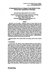
to determine the roll bias. As the ship conducts the survey at the ocean field, the multibeam sonar was continuously moving in respect to the ships motion. The data needs to be corrected for any bias introduced by the changing pitch and roll of the ship. Roll bias was a measure of the difference between the atwartship alignment of the ship’s multibeam hydrophone array, and that of its vertical reference source” [2]. The roll and pitch bias values for each region of the survey are determined by using the mbrollbias and mbpitchbias programs. Two segment lines of the data are selected as input files into the mbrollbias. The program calculates the bias correction for that region and through mbset applies it to the entire data set. High quality multibeam sonar data requires an accurate measurement of sound velocity profile (SVP). Sound travel in the ocean can different effects on the data. MB-systems had programs such mbvelocity tool and mblevitus for calculating a new SVP. Multiple sources of data can help determine the correct SVP. MbLevitus provides a historical database for which it creates a SSP. During the survey, accurate sound speeds and depths were inputted into the EM120 data through direct measurements. Using mbvelocity tool the direct measurement and mblevitus historical SVP’s were loaded and manipulated in real time; a new SVP was created for the data set. Hereby the listing program of MB system software. Figure 1 and 2 showed the flow of data processing procedures before correction Figure 3 is the flow of data analysis procedures after correction and Figure 4 show the data analysis procedures to get maps and graphics in Windows file type.

A

Figure 1. Data Processing Procedures for Correction

146



A

A

Figure 2. Data Analysis Procedures for Correction

A

B

Figure 3. Data Analysis Procedures for Total Correction


147


B

Figure 4. Data Analysis Procedures to Get Maps and Graphics in Windows File Type Raw.all data format were processed in the MB System on a Linux based computer to produce bathymetric profile and amplitude (backscatter) of sea bottom. The next step is to save all data in a single file raw.all file. Processing of data on MB System begins with a repeater of the overall data contained in a single file with a file using the ls command. Datalistraw.all could be processed to map the path the ship when collecting data, bathymetric maps and map the distribution of backscatter bottom waters that have not undergone a process of correction which is set in the command mbm_plot as below:  ls | grep .all $ > list.mb-1  mbm_plot –F–1 –Ilist.mb-1 –G2/G4/N –Ooutputfilename –L”judulpeta”:”judullegenda” –T –MGQ300 –MTG50 –MTIa –MTNa –PA4 –U1

The next stage was to perform data format conversion from .all to . * ID mb57 from the command mbcopy. Data of statistics file ( . * Inf ), fast bathymetry (. * FBT) and fast navigation (. * FNV) first extraction of a repeat * Mb57 with mbdatalist command. Correction value of the amplitude of the angle of the data (grazing angle ) formed by any subsequent correction process beam used mbbackangle command. This correction to apply calculations on across track slope of the bottom surface waters and type of grid used as a sweep of the area topography factor to calculate the grazing angle at each point of the data. The correction is performed twice by applying two angles in reference to the entire amount of data using the value sonar pings and average altitude. Reference angle used was 300 and -300 on different sides of the beam and carried out in two rounds of data using mbprocess . The result of this correction are two files with the data format .mb57 . * Aga for each data and datalist.mb - 1_tot.aga . The syntax of program as shown below:

148



 mbm_copy –F57 –Ilist.mb-1  ls | grep .mb57 $ > datalist.mb-1  mbdatalist –F–1 –Idatalist.mb-1 –N –V  mbotps –F–1 –Idatalist.mb-1 –D60 –M  mbbackangle –Idatalist.mb-1 –A1 –Q [–Tgrid] –V  mbset –PAMPCORRFILE:datalist.mb-1_tot.aga  mbset –Idatalist.mb-1 –PSVPFILE:SO189-1-CTD20060815.asvp –PDRAFT:6.8  mbvelocitytool  mbeditviz

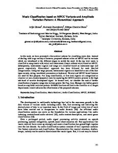
Sound velocity profile (SVP) was corrected by computing the data recording by SeaBird simultaneously with SVP height in the water vessel (draft) as a reference depth multibeam devices with mbset. Digitization between SVP pattern obtained from the Seabird and average speed of sound was applied using MB system of mblevitus . The correction was done through the display mbvelocity tool and directly applied to the data. The results indicated by the change in the beam sweep region or beam coverage and beam residuals at each beam number (Figure 5 and 6).

Figure 5. MB-systems Using Mbvelocity Tool before Sound Speed Correction

Figure 6. MB-systems Using Mbvelocity Tool after Sound Speed Correction This process ends with the appearance of the file with .mb57 format. Correction using mbeditviz for beam forming of seabed topography was conducted in three dimensional (3D) editing sounding. Therefore, the outer beam and the tenuous beam can be calculated, because the speed of sound in water changes (Figure 7 and 8). Errors in multibeam sonar systems are predictable [2]. Mbclean provides many options for flagging data depending on survey area. The most common option was to flag a number of specified outer beams


149


from both sides of the sonar array. Sound speed profile errors are usually larger in the outer beams along with a low signal-to-noise ratio (SNR). The syntax of the program as shown below:    

mbset –Idatalist.mb-1 mbprocess –F–1 –Idatalist.mb-1 ls | grep p.mb57 $ > datalist2.mb-1 mbgrid –A2/A3 –N –Idatalist2.mb-1 –Ooutputfilename –E100/0/m! –F5 –Rkoordinat –M

 mbbackangle –Idatalist2.mb-1 –A1 –Q [–Tgrid] –N191/65 –P2196/1822 –R30 –Z895.37/4668.72 –V  mbset –PAMPCORRFILE:datalist2.mb-1_tot.aga  mbprocess –F–1 –Idatalist2.mb-1  ls | grep pp.mb57 $ > datalist3.mb-1  mbbackangle –Idatalist3.mb-1 –A1 –Q [–Tgrid] –N191/65 –P2196/1822 –R–30 –Z895.37/4668.72 –V  mbfilter –A1 –F–1 –S2/3/3/1 –Idatalist3.mb-1  mbmosaic –A3 –Idatalist2.mb-1 –F0.1 –C10 –N –Ooutputfilename  mbgridviz  grdmath survey-datalist_sd.grd survey-datalist.grd DIV 100 MUL \ = survey-datalist_sdpercent.grd  mbm_grdplot –I –G2 –W1/2 –S(optional) –L”judulpeta”:”judullegenda” –T –MTIa –MTNa –PA4 –U1 –S -MGFl  csh mbgridoutputfilename  mblist –Idatalist3.mb-1 –F–1 –MA –OTXYZ

Figure 7. Profil of Seabed Using Mbeditviz

Figure 8. Profile of Bathymetry in 3d Soundings

150



The overall correction was then applied to the data using the command mbset inside datalist of * Mb57. Data processing using mbprocess performed on MB System to obtain files containing overall correction to all the data. Gridding process using mbgrid command was performed to define the type of data, the type of gridding and coordinate gridding and file name issued after gridding process. The data type was set to be the topography and the amplitude of the type of gridding on mbgrid using weighted sonar footprint. Gridding type of beam width calculated based on the angle that form and movement sonar sweep of the area above the sea floor. Large depth variations still produces high resolution using the gridding types because the algorithm has a good sensitive result in shallow waters or in waters within cells because it has gridding smaller than the width of the sonar sweep. Weighted footprint suited with amplitude correction to the grazing angle using slope factor base surface waters in the area perpendicular to the vessel. Further processing after the application of the angle in which the values of the amplitude of the low pass filter using mbfilter command with a Gaussian filter types mean for the low pass filtering before united through mbmosaic. Gaussian mean attention to the frequency content of the data was better than other methods. Low pass filtering will be set aside outlayers maximum values were not entered into the class division of the histogram value. Syntax of mbmosaic scattering was used to perform basic amplitude data gridding waters has twice suffered a correction to mbbackangle. Gridding on mbmosaic case with mbgrid, but the command was devoted to the processing of amplitude values and grazing angle of multibeam echosounder. Assigning a priority value on mbmosaic with Gaussian weighted mean mosaicing made the data appear regardless of the values of outliers (outlayers). Gridding results can be checked through the 3D view by using mbgridviz. Appearance and usability mbgridviz basically was the same as mbeditviz. Mbgrid with additional command code was used to calculate the density of the beam and the statistical standard deviation of the depth. Statistical maps of standard deviation as a percentage of the depth of water that shows the accuracy of the data based on the depth obtained through grdmath. The functions of map display such as colorbar, colormap , resolution and size of paper set in mbm_grdplot. Getting a map view that corresponds to the class histogram created by mbsystem using code so that the values outlayers ignored. The next step was the execution of the map file to be displayed with the csh command and data extraction parameters of multibeam echosounder. Data parameters were corrected in the form of * .txt.

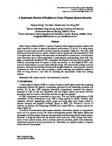
4. Results and Discussion Total acoustic data held was 178 225 ping with 98.54 % of the data recorded with good beam and 1.46 % do not have a value or zero beam for all bathymetric data and amplitude. Minimum depth along the path of the survey is 31.19 meters and a maximum at 5167.59 meters with the lowest amplitude value is -55.5 dB and 21.0 dB highest obtained from raw multibeam echosounder. Slope area was on the track BGR06-207 with coordinates of 94.762667187 94.929630834 BT and 2.236548207 - 2.849371539 LU. The length of the study area was 67.0779 kilometers and reached for 2.3633 hours. Total echo examined were 1822 348 002 ping and beam points beam of 191 numbers. Total beam corrected to shape local profile slope as much as 85.79 % and 0.66 % classified as zero beams and 13.55 % classified as flagged beams for all bathymetric data and amplitude (Figure 9). Simeulue basin area on the track BGR06-212 with coordinates of 95.744591884 95.983490060 BT and 3.105014649 - 3.286205689 LU. The length of the study area was 29.4923 kilometers and reached for 2.9986 hours Total echo examined were 2196 419 436 ping and beam points beam of 191 numbers. Total beam corrected to shape the profile of Simeulue Basin area as much as 99.72 % and 15.0 % classified as zero beams


151


and 0.28 % classified as flagged beams for all bathymetric data and amplitude (Figure 10).

(a)

(b)

Figure 9. Profile Bathymetry (A) And Standard Deviation (B) Of Slope Area

152



(a)

(b)

Figure 10. Profile Bathymetry (A) And Standard Deviation (B) Basin Area Of Simeulue Minimum depth of the slope area of 813.59 meters and a maximum at 4904.71 meters while the basin area of 723.01 meters to 1065.21 meters. Sweep width changes in slope areas due to beam spreading perpendicular to the axis of the vessel (acrosstrack) as the depth increases. Retrieving data using an angle of 650 as beam angle from the bottom with a maximum width using IHO 2008 criteria. Slope and basin area of Simeulue Island was included in the order 2 with a horizontal accuracy of 20 meters plus 10 % of the current depth measurement. Figure 10b showed the standard deviation as a percentage of water depth. This value was the result of standard deviation divided by the depth of the depth value is then multiplied by the overall. In the slope area, MBES had a noise level of 0 % to 3.75 %,


153


which represents the standard deviation value of depth error to the overall depth of sea water. Noise in this area averaged at a value of 0 % to 1.5 %, and the maximum noise with a value of 3.75 % in the area that does not wide area. Figure 10b showed standard deviation as a percentage of the depth of the waters of the basin area. In the basin area a noise level of 0 % to 1.75 %. Noise in this area averaged at a value of 0 % to 0.52 %, and the maximum noise with a value of 1.75 %. The appearances of noise on the MBES were caused of the condition of the sea, electrical interference on the equipment, and the noise of the ship when the data collection takes place [13]. The value of standard deviation as a percentage of the waters depth was lied on high slope area and steep topography, while the area of the basin has a value in the area near the bottom and outer side beam. Topography is due to changes in shape with increasing depth and use the SVP value less precise. The backscatter obtained and processed from three zones in one sweep the beam specular zone, oblique and grazing. Specular zone or mirror like located at the nadir (00 150 in the processing in MB - System) will have a value of backscatter was very strong or high intensity. Oblique angle is in the range of 100 to 200 or 500 or 600 outside the zone of specular and have the backscatter was medium intensity and these values were used to measure the roughness and volume of sediment. Grazing zones located on the outer beams that is more than 600 with the low backscatter and used to obtain the bottom roughness [10]. Backscatter signal received by MBES systems could be affected by several parameters such as instrument settings like transmitter power, the signal is received, and the pulse length , the propagation of the acoustic signal (attenuation and dispersion), geometric beam (distance, angle formation, size footprint ) and the characteristics of seawater. The effect of the geometrical beam angle, the more difficult to be removed particularly in specular zone [11-14]. Figures 11 and 12 showed the distribution of backscatter on the slope and basin areas. Figures 11a and 12 show a correction on the amplitude, the grazing angle, and without using reference angle. Slope area had a value of minimum amplitude -43.90 dB and maximum at 14.30 dB with a maximum value of 16 dB outlayer and minimum of -46 dB outlayer. While in the basin area had the minimum amplitude -44.29 dB and a maximum of -3.58 dB with a maximum value of 11 dB outlayer and minimum of -53 dB outlayer. Regional nadir parallel with the axis of the track ships and boats ( alongtrack ) produces rare stripping shown in red that has a maximum value of 14.30 dB on the slope and -3.58 in the basin. In Figure 11, there was shown a shift in the nadir that was not aligned with the path of the ship (alongtrack) in the box dashed black. It was caused by the roll bias that occurs at the time of data collection vessel and influence the bottom backscatter. Figure 13 and 14 showed the relationship between the number of beam and the value of backscatter before and after correction using MB System. Beam number from 0-94 shows the port side (left side of the boat) and 96-190 shows the starboard (right side of the boat) with a beam number 95 as indeed was the nadir point 0. Backscatter at nadir value 00 (incidence angle 00 or 900 of grazing angle), beam number 95 and specular areas with beam number 80-100 in the region backscatter slope has a positive value. Based on the relationship shown the angle of incidence of the pattern of the acoustic signal determines the maximum value of the entire sweep of the area. This was caused by the length of the horizontal side at the bottom that receive acoustic signals, specular area ( vertical incident ) will be more likely to have the number of long horizontal sides and the bottom waters are effectively able to reverse the acoustic signal coming [11]. Nadir stripping can be overcame by applying the correction reference angle when the amplitude value of the grazing angle and perform filtering and backscatter mosaic process on the data. Then, the effect of the positive value of the amplitude (backscatter) can be minimized. Angle of 300 was the default in the MB System when used in order correction. Value of backscatter on the incident angle 300 had a maximum value that can be compensated for the specular zone and the minimum value to compensate for the data

154



processing in grazing zone. Using mbprocess, the backscatter value in the reference angle was used as a reference in the formation of backscatter value previously been applied through mbbackangle.

(a)

(b)

Figure 11. Profile of Amplitude Value before (A) And After (B) Applied Reference Angle, Low Pass Filter


155


Figure 12. Distribution of Amplitude after Applied Reference Angle, Low Pass Filter and Mosaic

Figure 13. Beam Number and Backscatter before Correction

156



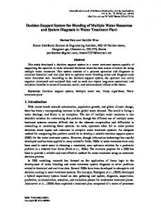
Figure 14. Beam Number and Backscatter after Correction Figure 15 showed a significant change occured in the backscatter after the application of reference point conducted. The backscatter of specular zone was lower than before the implementation of the reference angle. Backscatter of oblique and grazing zones were gained on the maximum found using the reference angle application. These phenomenon were caused by the bottom roughness and the backscatter in the specular zone compensated for other zones. Our result was suitable with the Lurton research using multibeam echosounder [6]. Figures 15a and 15b showed a clearly spread of backscatter after reference angle application. Slope area had a minimum value of the amplitude of 42.37 dB and a maximum of -4.47012 dB, meanwhile the basin area had the minimum amplitude of -41.5992 dB and maximum -16.63 dB. (a)


157


(b)

Figure 15. Pattern of Backscatter and Incident Angle in the Slope Area (A) And Basin Area (B) After Applying the Reference Angle

5. Conclusions This research had developed and applied the MB system software to processed and analyzed the acoustic signal from multibeam echosounder. The bathymetry and backscatter distribution maps were computed after tidal correction process, amplitude of the grazing angle, the sound velocity profile, editing 3D bathymetry, low pass filter and mosaic amplitude. The depth values of the slope area were 813.59 meters to 4904.71 meters and at basin area were 723.01 meters to 1065.21 meters depth. Backscatter distribution maps using the reference angle, low pass filter and amplitude mosaic yield a range of values of backscatter without stripping nadir. After the reference angle applied, the minimum amplitude of bottom backscattering strength was -42.37 dB and the maximum value was -4.47 dB in the slope area, while in the basin area were -41.59 to 16.63 dB dB.

Acknowledgements The authors were gratefully thanks to researchers of Research Vessel (RV) SONNE owned by RF Forschungsschiffahrt GmbH, Bremen, Germany and Agency for Assessment and Application Technology Indonesia for collecting the field data.

References [1] [2] [3] [4] [5]

[6] [7] [8]

158

J. D. Beaudoin, J. E. H. Clarke and J. E. Bartlett, Retracing (and Re-raytracing) Amundsen’s Journey through the Northwest Passage. Canada, (2003). D. Caress, D. Chayes and V. Schmidt, The MB-System cookbook, (2010). IHO, Standards for Hydrographic Surveys Monaco: International Hydrographic Bureau, (2008). “Kongsberg Maritime”, Product Description: EM 120 Multibeam Echo Sounder, Norwegian: Horten, (2005). S. Ladage, “Simrad EM120 multibeam bathymetry system”, Research Cruise SO189 Leg 1 SUMATRA: The Hydrocarbon System of the Sumatra Forearc, Hannover: Federal Institute for Geoscience and Natural Resources, (2006), pp. 33-35. X. Lurton, An Introduction to Underwater Acoustics, Springer, (2002). X. Lurton, “Backscatter measurement by seafloor-mapping sonars: basics and challenges”, GEOHAB Workshop Perancis: Underwater Acoustic Dept, (2013). L. A. Mayer, “Frontiers in seafloor mapping and visualization.Mar. Geophys. Res., vol. 27, (2006), pp. 7-17.



[9] S. Neben, “Navigation and Positioning”, Research Cruise SO189 Leg 1 SUMATRA: The Hydrocarbon System of the Sumatra Forearc, Hannover: Federal Institute for Geoscience and Natural Resources, (2006), pp. 33-35. [10] I. M. Parnum and A. N. Gavrilov, “High-frequency multibeam echo-sounder measurements of seafloor backscatter in shallow water: Part 2 – mosaic production”, analysis and classification. International Journal of the Society for Underwater Technology, Perth: Curtin University, vol. 30, no. 1, (2011), pp. 13–26. [11] I M. Parnum, A. N. Gavrilov, P. J. W. Siwabessy and A. J. Duncan, “The effect of incident angle on statistical variation of backscatter measured using a high-frequency multibeam sonar”, Proceeding of ACOUSTICS. Australia Barat: Busselton, (2005). [12] I. M. Parnum, A. N. Gavrilov, P. J. W. Siwabessy and A. J. Duncan, “Identification of seafloor habitats in coastal shelf waters using a multibeam echosounder”, Proceeding of Annual Conference of the Australian Acoustical Society, Australia Barat: Gold Coast, (2004), pp. 181-186. [13] P. J. W. Siwabessy, A. N. Gavrilov, A. J. Duncan and I. M. Parnum, “Statistical analysis of highfrequency multibeam backscatter data in shallow water”, Proceeding of ACOUSTICS New Zealand: Christchurch, (2006). [14] V. Schmidt, D. Chayes and D. Caress, “The MB-System Cookbook”, Columbia University, (2005). [15] T. K. Stanton, “30 years of advances in active bioacoustics: a personal perspective”, Methods Oceanogr., vol. 1-2, (2012), pp. 49-77.

Authors Henry M. Manik, he received the B.S degree in Marine Science and Technology Department in the field of Marine Acoustics from Bogor Agricultural University Indonesia in 1994. Master of Techniques (M.T) degree in Geophysical Engineering Department in the field of GeoAcoustics from Institute of Technology Bandung Indonesia in 1999. He also received Ph.D degree of Marine Science and Technology in Underwater Acoustics Engineering from Tokyo University of Marine Science and Technology, Japan in 2006. Since 1997, he has been a lecturer and researcher in Department of Marine Science and Technology Bogor Agricultural University Indonesia. His current research interests include underwater acoustics propagation, ocean instrumentation, sonar and seismic signal processing and acoustic backscattering from marine biota and seafloor. Diandra Yulius, he has been the B.S student in Marine Science and Technology Faculty of Fisheries and Marine Science Bogor Agricultural University Indonesia. His current research interest include multibeam processing and underwater robotics

Udrekh, he received the B.S degree in Geophysics from Institute Technology Bandung Indonesia. He also received M.S and PhD degrees from the University of Tokyo, Japan. He worked at the Agency for the Assessment and Application Technology Indonesia. His current research interests include geophysical mitigation and seismic processing.


159


160


Journal Paper Format - SERSC

Journal Paper Format - SERSC

Suggest Documents