JPEG2000 as possible, we discuss some issues in coding transform coefficients resulting from ... non-scalable coding at the highest of the embedded rates.
JPEG2000-based Scalable Video Coding with MCTF Peter Eder
Dominik Engel
Technical Report 2007-04
Andreas Uhl
October 2007
Department of Computer Sciences
Jakob-Haringer-Straße 2 5020 Salzburg Austria www.cosy.sbg.ac.at
Technical Report Series
JPEG2000-based Scalable Video Coding with MCTF Peter Eder, Dominik Engel, and Andreas Uhl Department of Computer Sciences University of Salzburg, Austria {peder,dengel,uhl}@cosy.sbg.ac.at
Abstract. We discuss the possibilities and limitations of a scalable video codec based on JPEG2000. We give a review of wavelet-based motion-compensated temporal filtering (MCTF) and discuss how JPEG2000 components can be used for coding temporal subbands and motion data. At the example of a simple implementation that uses as many ingredients from JPEG2000 as possible, we discuss some issues in coding transform coefficients resulting from MCTF. We also discuss to what extent JPEG2000 can be used to encode motion vector data in a lossless way. Finally, we present some compression results that can be achieved by putting the simple ingredients together, and compare them to MPEG-2 and MC-ECBZ, a “proper” wavelet-based scalable video codec.
1
Introduction
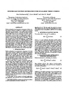
In recent years the consumer applications in the field of multimedia have become increasingly heterogeneous. A multitude of different end-clients exist, all with different capabilities in terms of computing power and display capacities. Scalable video coding makes it possible to encode visual content only once for use with a large range of different display devices with varying resolutions and capabilities. The same bitstream can be used to serve home-cinema quality content in HDTV resolution, full quality and full framerate or a mobile client with low computational power in QCIF resolution, reduced quality and a fraction of the original framerate without the need for re-encoding. Adaptation can also happen during transmission: A scalable bitstream can be adapted to fit heterogeneous conditions in different networks, satisfying the demands of an error-prone wireless network, satellite-links with large round-trip times or high-fidelity fiber-optic wired networks with high throughput. Three common types of scalability are usually distinguished: resolution (or spatial) scalability, quality (or SNR scalability) and temporal scalability. Figure 1 illustrates the types of scalability. The overhead that is introduced by scalable coding should be as small as possible in comparison to non-scalable coding at the highest of the embedded rates. With the addition of the scalable extension to H.264/AVC, ITU-T and MPEG have responded to the need for a standard in scalable coding (see, e.g., [1]). The scalable extension of H.264, H.264 AVC/SVC, is in many ways compatible to non-scalable H.264, and the introduced overhead is relatively small (in some settings, the scalable variant outperforms non-scalable H.264, because some methods have improved since H.264 was standardized). In the call for proposals for this scalable extension, a major part of the submission were waveletbased. In the end the non-wavelet-based submission that was the closest to the non-scalable version of H.264 won the race. This is a sensible move, as the method delivers scalability at low overhead cost, while retaining a close resemblance to non-scalable H.264. 1
original video sequence
encode
scalable video stream
decode
qualitative scalability
spatial scalability
temporal scalability
Fig. 1. Three Types of Scalability
However, the wavelet-based approaches merit a second look even after SVC has become a standard. Wavelets inherently provide dyadic spatial scalability. Also for quality scalability waveletbased coding is very well suited, as can be seen in JPEG2000, the scalable standard for still-image coding [2]. Finally, with motion-compensated temporal filtering (MCTF) wavelet-based video codecs support temporal scalability. The idea of motion-compensated temporal filtering actually stood at the beginning of what is now H.264/AVC SVC. The authors of [3] point out that the powerful concept of hierarchical B-pictures is equivalent to motion-compensated temporal filtering that leaves out the update step. In this paper we will investigate the potential of using the JPEG2000 coding engine for a scalable video codec. Thereby we try to use as few additional techniques as possible. The rationale behind this is to largely stay compatible with the JPEG2000 building blocks, which is a benefit when it comes to hardware implementations for example. Note that the following is a study of feasibility that does not aim to produce a competitive codec but rather aims at comparing some basic techniques. [4] report results from a similar project, although their codec is far more progressed than the concatenation of loosely connected experiments we report on in this paper. While we have only looked at certain parts of the coding chain in detail and have left other parts, e.g. rate-distortion optimization, at a rudimentary level, they have built an elaborate JPEG2000-based scalable video codec that, in some settings, is competitive with H.264. However, our report may give a different perspective on some topics, and, in the case of MV-coding, may even go a step further than the codec presented by [4]. The rest of this paper is organized as follows. In section 2 we give an overview of MCTF waveletbased scalable video coding, in Section 3 we discuss the collection of techniques we investigated for 2
temporal filtering, residual coding and motion vector coding. Results and a comparison to MPEG-2 and MC-EZBC are presented in Section 4. Section 5 concludes.
2
Wavelet-based Motion-compensated Temporal Filtering
Many contributions have been and are mad to the field of wavelet-based t+2D MCTF. Motioncompensated embedded zeroblock coding [5] (MC-EZBC) performs MCTF first followed by EZBC entropy coding. It allows for fractional pixel accuracy and overlapped block motion compensation. A good overview of MC-EZBC (and MCTF in general) can be found in [6]. Ohm and coworkers, whose early proposals form the basis of wavelet-based video codecs [7], have also made a number of substantial contributions to the subject of wavelet-based scalable video coding, see for example [8]. Another group of researchers focus on in-band MCTF, i.e. the 2D+t variant, see [9]. [10] is a joint publication by members of these three groups that provides a good overview of 2D+t and t+2D wavelet-based MCTF techniques. In [11], MC-EZBC is compared to 2D+t in-band MCTF and another variant of t+2D spatial-domain MCTF. In the area of wavelet-based scalable video coding related to JPEG2000 coding, apart from the aforementioned proposal ([4]), there are also proposals from Taubman and coworkers: In [12], a wavelet-based scalable video codec is proposed that uses many techniques of JPEG2000 coding. Once finalized, JPEG2000 Part 10, [13], which deals with 3D data coding, although targeted at volumetric data, could also present an interesting option for video coding. In the following we briefly review the basic concepts of wavelet-based MCTF. For a detailed account, refer to e.g. [10, 8, 6]. The idea of wavelet-based motion-compensated temporal filtering is to remove redundancies between frames by performing a wavelet transform along the temporal axis. Thereby the filtering is performed along previously determined motion trajectories in order to utilize movement in the source video. Two major groups of approaches can be distinguished: 2D+t and t+2D. 2D+t approaches start by doing a wavelet transform on the frames. The temporal filtering follows. Some difficulties arise for these approaches with the motion estimation: because the spatial filtering is done prior to the temporal filtering, motion compensation has to be performed in the wavelet domain. t+2D approaches perform the temporal filtering first, and then do spatial filtering on the resulting temporal subbands. Therefore t+2D approaches can do motion compensation in the spatial domain. They can draw on the resources of available knowledge on motion compensation in the spatial domain. In this paper we choose this t+2D approach for our investigation. The basic operation is illustrated in Figure 2 for a temporal decomposition level of 3 with the Haar filter. First motion compensation is performed on the 8 input frames in non-overlapping, consecutive pairs (green arrows). Then, to obtain the first temporal decomposition level, the 8 input frames are filtered along the motion trajectories with the Haar filter in pairs. As a result we get 4 temporal lowpass and 4 temporal highpass frames. Much like in the spatial wavelet transform the 4 temporal lowpass frames are used for further decomposition. Note that motion compensation is performed again for this temporal decomposition level. The MCTF process is repeated until we have the single temporal subband of lowest resolution (LLL in our example). We will discuss the properties of this subband further below. Note that if a lifting implementation is used for temporal filtering, then the motion compensation can easily be integrated into the lifting steps, as illustrated by Figure 3 for the Haar wavelet: the input frames are taken in pairs (each of which consists of an even frame A and an odd frame B). Each position in the highpass frame H is constructed by subtracting the corresponding, motioncompensated position from frame B. The lowpass frame L is constructed by adding to the original 3
A
B
A
B
A
B
A
motion compensation
video sequence motion vectors
B
temporal filtering
spatial filtering L
temporal filtering
H
spatial filtering LL
LH
temporal filtering spatial filtering LLL
LLH
Fig. 2. t+2D Scalable Video Coding (from [8])
position in B the motion-compensated position in frame B multiplied by 0.5, although this time using the inverse motion-compensation. Thereby the transformation can be done in-place. The temporal filtering results in 8 temporal subbands: one low-pass subband and seven subbands containing higher frequencies. In the next step, spatial filtering, a 2D wavelet filter (e.g. CDF 9/7) is applied to these 8 subbands. After MCTF, usually quantization and entropy coding are performed (in our case, using the JPEG2000 coding engine). Of course, the motion data that is created during MCTF has to be encoded in the output bitstream as well. In our example, seven motion vector fields are needed. With longer filters the amount of motion data will increase. Conceptually we have a motion vector for each pixel, although often sets of motion vectors will be coded as blocks. Depending on the size of the search range, the dynamic range of the coordinates of the motion vectors will vary. A larger search range will result in larger, and often more inhomogeneous, motion vector fields with a larger entropy. The trade-off between spending many bits on motion vector coding versus using these bits for the coding of visual data is a point with a lot of potential for improvement. In any case, the efficient coding of motion data is crucial, and we will discuss this point in Section 3.2. 4
A
B
A
B
MC 1
A
MC
−1
1
H
IMC
1
L
B
MC
−1
1
H
IMC 1
A
MC
−1
H
1/2
B
H
IMC
1/2
1
L
−1
IMC
1/2
1
L
1/2
1
L
Fig. 3. Lifting-integrated motion-compensation (from [8])
The subbands resulting from the MCTF can be seen as a 3-dimensional cube of wavelet coefficients. Depending on which portion of the cube is taken, different kinds of scalability can be realized, as illustrated in Figure 4. For spatial scalability the data is cropped along the horizontal and vertical axes. For temporal scalability, along the temporal axis. Quality scalability can be realized by refinement coding of the wavelet coefficients. The portion of the cube taken in the example of Figure 4, highlighted in green, corresponds to the data needed for CIF-resolution at 30 frames per second.
3
JPEG2000-based SVC
In the following we discuss some issues of MCTF-based video coding based on JPEG2000. One of the aims is to stay as close to JPEG2000 standard as possible. Therefore, we investigate the feasibility of coding the wavelet coefficients and the motion vector data with JPEG2000. Figure 5 shows the block diagram of the coding pipeline. Motion Estimation is performed on the input data. The resulting motion vector fields are used to perform motion-compensated temporal filtering on the input data. Transform Coefficients and motion vector data are both coded using (parts of) JPEG2000. The rate allocation uses this information to control tier-2 coding of JPEG2000. Finally, a scalable bitstream is produced. 5
60 Hz
30 Hz 15 Hz 7.5 Hz
CIF
SD
HD ver
QCIF
p
m
hor
te
Fig. 4. 3D Wavelet Cube (from [8])
The basis for our implementation was formed by version 4.1 of the JJ2000 reference implementation1 .
3.1
Motion Compensated Temporal Filtering
Motion estimation is one of the modules that we only investigated peripherally. In our experiments we use a conventional (non-overlapping) block matching algorithm that minimizes the mean square error as distortion criteria. The estimation is done at full pixel accuracy. The parameters for macroblock size and the size of the search window can be chosen. For the compression of the temporal subbands, in addition to the lossy mode, we also added a lossless mode, both of which we discuss in the following.
Lossy Mode For lossy compression we do motion-compensated temporal filtering using the Haar wavelet. Let s be the lowpass signal, d be the highpass signal, and x be the input signal. The lifting steps (without motion compensation) for the forward transform with the Haar wavelet can 1
http://jj2000.epfl.ch/
6
Rate Allocation MV Data
JPEG2000
MCTF Input Data
Transform Coeffients
SVC−Bitstream Writer
Motion Estimation
Output
Fig. 5. Overview of the Coding Pipeline
be written as follows [14]: (0)
(1)
sl
= x2l
(0) dl
= x2l+1
dl =
(0) dl (0)
sl = sl
(2) (0) sl
(3)
1 + dl 2
(4)
−
and the inverse transform can be written as: (0)
sl
(0)
dl
1 = sl − dl 2 (0) = dl + sl
x2l+1 = x2l =
(0) dl (0) sl .
(5) (6) (7) (8)
As described above, the input frames are processed in pairs. Let each pair consist of the even frame A and the odd frame B. In our implementation, motion compensation is done from B to A, i.e. for each macroblock in B, the best macroblock in A within the offset defined by the search window size is determined by minimizing the MSE between all candidate blocks. The highpass lifting steps computes the difference for each position in frame B with the motion-compensated position in frame A. This difference is written to the position in frame B. The lowpass lifting steps works from frame A to frame B. We could do a full motion estimation from A to B again, and the transformation would still be reversible. The problem with this approach is that it suffers from inferior energy compaction while at the same time having to transfer an extra motion vector field. In order to have a reversible transform that also performs reasonable energy compaction, we therefore need to reverse the motion vector field that was computed in the highpass lifting step. Another advantage, except for the necessary property of energy compaction, is that we 7
only need to transmit a single motion vector field, because with this information the decoder can also do the inversion. Some positions in B may be referred to by more than one position in A (multiply connected ) and other positions in B may not to referenced at all (unconnected ). These two special cases have to be considered in the lowpass lifting step. There are different propositions how to deal with these cases; we follow the proposition by [10]: For unconnected positions, the value of A is used as the output of the lowpass lifting step. For multiple connection, any of the positions in B that refer to the position in A may be used in the lowpass lifting step. In our implementation we use the first (a more sophisticated implementation could use the shortest motion vector). The lowpass lifting step subtracts half the value of the position at B from the position at A. After temporal transformation, the temporal transform coefficients are encoded with JPEG2000 using the CDF9/7 filter. For a competitive codec, at this point, proper rate-distortion optimization is crucial. An interesting option would be to use the R-D optimization of JPEG2000 for codeblocks on the 3D cube of wavelet coefficients of each group of pictures. As our focus is not on rate-distortion optimization, we only use a very crude rate allocation to the temporal frames: we assign two different rates for the coding of the coefficient data, one (usually higher) rate for the approximation subband and one (lower) rate for the detail subbands. The trade-off between motion data and coefficient data is not considered at all. With this crude rate allocation, however, we get a rough control over the size of the final bitstream, which allows us to compare the compression performance of different configurations. For a sophisticated approach to rate distortion optimization, see [4]. Lossless Mode The lossless mode was added mainly for verification purposes. For the lossless mode we use an integer variant of the Haar filter for temporal filtering. Let s be the lowpass signal, d be the highpass signal, and x be the input signal. The lifting steps for this filter can be written as follows. The forward transform is changed to (0)
sl
= x2l
(0) dl
= x2l+1
dl = sl =
(0) dl (0) sl
(9)
−
(10) (0) sl
(11) (12)
and the inverse transform is changed to (0)
sl
(0) dl
= sl = dl +
x2l+1 = x2l =
(0) dl (0) sl .
(13) (0) sl
(14) (15) (16)
As the update step only consists of retaining the image value of the left frame, after the transformation, in the lowpass temporal subband we have the first (leftmost) frame of the group of pictures. The other frames contain the residuals. The temporal subbands are spatially filtered using the 5/3 lossless integer filter of JPEG2000. Together with spatially predictive MQ motion vector coding using Exponential Golomb Codes, as described below, lossless compression is achieved. 8
3.2
Motion Vector coding
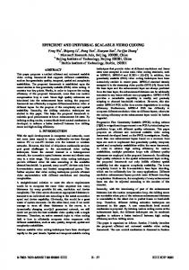
Apart from the transform coefficients, motion data is the second set of data that has to be encoded. In order to stay as close to JPEG2000 as possible we chose as an initial approach to code the motion vector fields with JEPG2000 in lossless mode. This idea was first suggested by [15]. In [16], the performance of coding motion data with JPEG2000 with different configurations is evaluated. In [15], the authors split each motion vector field into its horizontal and vertical components. Large motion vector images are constructed for all horizontal and all vertical components, respectively. These are then encoded with JPEG2000 without wavelet decomposition. The authors tested spatial and temporal prediction schemes to improve performance but conclude that the configuration without prediction “proved to be the most robust while being the simplest” [15]. The same approach is also used in [17]. Presumably, [4] uses this approach as well, but the authors remain a little vague here and only mention that “[t]he motion information is encoded losslessly using EBCOT”. For our approach, we also experimented with different encoding strategy that use more or fewer components of JPEG2000. At first we tried the most straightforward approach: each motion vector field is split into its horizontal and vertical components (like in the approach proposed by [15]), each of which is coded as a separate grayscale image. The full JPEG2000 header information is written for each motion vector image. The coding performance of this approach turned out not to be competitive. This is illustrated by Figure 6: The number of bytes are shown that are spent for coding the motion vector data of the first group of pictures (temporal depth 3, i.e. 8 frames) of the Foreman sequence in QCIF resolution. Motion estimation was performed using full pixel accuracy, 8 × 8 macroblocks and a searchwindows size of 16 × 16. The leftmost box shows the number of bytes needed if the 7 motion vector fields are coded as JPEG2000 images in the described manner. It can be seen that the compression performance is weak by comparing the number of bytes to the rightmost box. The rightmost box in Figure 6 shows the number of bytes needed by the contextadaptive binary arithmetic coder (CABAC) of H.264, as described in [18]. This coder needs less than half of the bytes that the JPEG2000 image approach needs. We tried to improve performance of the simple approach by employing the spatial prediction scheme used by H.264. The result is shown in Figure 6 as the second box from the left. As can be seen, coding performance deteriorates with spatial prediction. JPEG2000 is not well suited to code the resulting residual data. As the full JPEG2000 header was coded for each of the images, we tried to increase coding performance by reusing JPEG2000 header data: the JPEG2000 main and tile headers were coded only for the first motion vector image. For the other motion vector images, we only code partial headers. This is similar to a multi-component approach. The resulting bytes needed can be seen in the third box in Figure 6 and while some savings were possible by decreasing the amount of header data, the performance of the motion vector image approach remains poor. The conclusion can only be that using the whole JPEG2000 coding pipeline (including a non-zero wavelet decomposition depth), which is tailored for good performance on visual data, to encode motion data, i.e. non-visual data, produces sub-optimal results. A better strategy than to use the full JPEG2000 coding pipeline is to only use the parts that are suitable for coding motion data. Such an approach would produce better results while still remaining as close to JPEG2000 as possible. We use the JPEG2000 MQ Coder to code the motion data. Essentially this is the same as done by [15], who use JPEG2000 with no wavelet transform to encode motion vector data. 9
4000 3750 3500 3250 3000 2750 2500 2250 2000 1750 1500 1250 1000 750 500 250 0
J2K w/o Prediction, all Hdr
J2K w/ Prediction, all Hdr
J2K w/o Prediction, partial Hdr
MQ w/o Prediction & EGC
MQ w/ Prediction & EGC
CABAC H264
Fig. 6. Comparison of bytes spent by different coding schemes for motion data (at the example of the first 8 frames of the Foreman sequence, QCIF, temporal decomposition level 3, full pixel accuracy, 8 × 8 macroblocks)
However, as H.264 performs very well at compressing motion data, we added some of the components from H.264 as described by [18]. One of these components is to use Exponential Golomb codes (EGC) to represent the motion vector data. We then encode these representations using the MQ Coder. The result is shown as the third box from the right in Figure 6. Although the coding performance is better than any of the JPEG2000 motion image approaches, it is still not convincing. Therefore as a final ingredient we add the spatial prediction used in H.264. The result is shown in the second box from the right, and it can be seen that with this setup the coding performance is comparable to H.264 motion data coding. The downside of using H.264 components is of course a deviation from the goal of staying as close to JPEG2000 as possible. In terms of compliance to JPEG2000 the approach proposed by [15] is preferable. The conclusion for motion vector data is that the MQ Coder can be used to obtain good compression performance. Thereby the choice of representation is vital. In our initial experiments we obtained good results with spatially predictive coding combined with Exponential Golomb Codes. Temporal prediction offers another possibility that could be investigated. Note, however, that each form of prediction potentially diminishes the extent of scalability in the final bitstream. For full scalability, a truly scalable format for motion vectors should be chosen. For more information on scalable motion vector coding, see [12, 19–21]. 10
4
Results
Our implementation is aimed at punctual experiments, like motion vector coding. Other parts of a (proper) video codec were not given much attention, such as motion estimation or rate-distortion optimization. Therefore it comes at no surprise that the concatenation of our experiments, which we will refer to as JJ-SVC, does not produce a coding pipeline that yields competitive compression results. Nevertheless, for the sake of completeness, in this section, we present some results and compare them to MC-ECBZ and MPEG-2. As has been detailed before, rate-distortion optimization is one of the main modules missing in JJ-SVC. In order to still give some compression results here we compressed test sequences with different settings for temporal decomposition depth, macroblock size and search window size. Furthermore we vary the rate for the temporal approximation subband and the temporal detail subbands. Some of these settings produce much better results than others at the same bitrate. We also add the results for JJ-SVC when no motion compensation is applied in the temporal filtering (this saves computational demands, but lowers compression performance). We compare the results of JJ-SVC with MPEG-2 and MC-ECBZ. MPEG-2 coding is performed by mencoder v.2:1.0 rc12 with the following options: -of mpeg -ovc lavc -lavcopts vcodec=mpeg2video -ofps 30. For MC-ECBZ we used full pixel accuracy only and no optimization. With optimization and fractional pixel accuracy the compression performance of MC-ECBZ is of course significantly higher than with these settings. Figures 7 to 11 show the compression performance of the four coders for five different test sequences. A frame rate of 30 frames per second was used, the sequences are 8bpp grayscale and have CIF resolution. In the case of MC-ECBZ and MPEG-2 the bitrates were chosen from 200 to 2000 kbps. In the case of JJ-SVC the bitrate was chosen as whatever the specified parameters produced. We used all possible combinations for JJ-SVC for the following settings of the individual parameters: – – – – –
temporal decomposition depths: 3, 4, macroblock size: 16 × 16, 32 × 32, 64 × 64, searchwindow size: 16 × 16, 32 × 32, 64 × 64, approximation subband rate: 0.5, 1, 5 bpp, and detail subband rate: 0.05, 0.25 bpp.
It can be seen that the performance of JJ-SVC is not a complete disaster, which is encouraging considering that very simple motion estimation is done and practically no R-D optimization is performed. There are actually a number of settings for which the coder produces acceptable results. Generally, these results are of course still not competitive. Only for the Highway test sequence some settings achieve a compression performance that is competitive with MPEG-2. Figures 12 to 16 show results for JJ-SVC per frame. The frames are plotted on the abscissa. For each frame three values are plotted: the number of bytes spent for video data (red), the number of bytes spent for motion data (green) and the achieved quality for each frame (blue). The range for the former two can be seen on the left-hand y-axes as the number bytes. The range of the latter can be seen on the right-hand y-axes as the PSNR in dB. Figure 12 shows the Foreman sequence with a temporal decomposition depth (TD) of 3. The bitrate for each temporal approximation subband is 0.5 bpp (LR) and for the each temporal detail subband the rate is 0.05 (HR). For the motion estimation a macroblock size of 8 × 8 pixels with a 2
http://www.mplayerhq.hu
11
search window of 16 × 16 pixels. The overall bitrate (OBR) achieved with this configuration is 528 kbps, the average PSNR (APSNR) is 30 dB. It can be seen that the first frame of each group of pictures has a higher visual quality than the other frames. This may seem surprising, as the temporal approximation subband represents the average of all frames in the group of pictures. However, as motion compensation is always performed targeted towards the left, the temporal approximation subband resembles the leftmost frame most and the rightmost frame least. Therefore, the lower frame rate for the temporal detail subbands, which can be seen as the residuals of the average approximation subbands to the respective frames, affects the frames on the left side more than the frames on the right side of the group of pictures. Note that this phenomenon can also be observed for MC-EZBC. It can also be seen that the camera panning motion that occurs in the last third of the Foreman sequence leads to a deterioration in visual quality as well as to an increase in the number of bytes spent on motion vector data. In Figure 13 we increase HR (the rate for the temporal detail subbands) from 0.05 to 0.25. The resulting increase in the overall bitrate is of course substantial: the overall bitrate achieved for this configuration is 1055 kbps. It can be seen in the plot that increasing the rate for the detail subbands flattens the decrease in visual quality for the frames on the right-hand side of each group of pictures. However, overall gain in PSNR is very low, considering that the bitrate is doubled: the average PSNR is 32.2 dB. In Figure 14 we show that the bitrate can be spent more intelligently, if the other parameters are tuned. With 1053 kbps the overall bitrate for this example is nearly the same like the last. We increase the macroblock size to 32 and the search window size to 64 × 64. LR is set to 1 and HR is set to 0.25. It can be seen that by decreasing the granularity of the motion vectors, the number of bytes spent on motion data also decreases significantly. These bytes can be spent on the visual part of the data. As can be seen the PSNR is generally higher, and the average PSNR is 35 dB. It can also be seen that the larger search window size reflects the panning camera motion in the last third of the sequence a little bit better than the short motion vectors of the previous examples. Figures 15 and 16 show some results for the Highway sequence. For both results a temporal decomposition depth of 4, i.e. a group of picture size of 16 frames, is used with a macroblock size of 32 × 32 and a searchwindow size of 64 × 64. The overall bitrate for Figure 15 is 251 kbps. It can be seen that even though the rate for the temporal detail subbands is quite low, the decrease in visual quality in each group of pictures from left to right is fairly limited. Giving a higher bitrate to both, temporal approximation and detail subbands leads to constant quality for Highway, as can be seen in Figure 16. The good performance is of course due to the uniform motion observed in Highway. Of course, many settings for JJ-SVC resulted in poor overall compression performance. Some used far too much data on the motion vectors, others spent all their bitbudget on the temporal detail frames and let the vital approximation subbands starve, leading to low overall PSNR.
5
Conclusion
We have reported on a series of experiments on different parts of JPEG2000-based MCTF video coding, mainly using very simple ingredients, as close to JPEG2000 as possible. We have shown for motion vector coding the MQ coder can achieve good results if the motion vector data is preprocessed with a simple spatial median predictor and represented with Exponential Golomb codes. We have discussed compression results for five different sequences, and have shown that in its present state the concatenation of these parts does not yield competitive compression results. 12
Concludingly, we can state that with the correct settings, compression results that are not all that far below MPEG-2 can be achieved. Of course, compared to recent compression standards like H.264 the compression performance is not competitive at all. But remember that some vital parts of the coding pipeline are missing. If these are fleshed out, like it is done in the codec by [4] there is a lot of potential for a JPEG2000-based scalable video codec: they report that their codec is competitive with H.264.
13
BUS-CIF 38 36 34
PSNR
32 30 28 26 24 22 20 0
500
1000
1500
2000
2500
kbps JJ-SVC, NO MC JJ-SVC, MCTF
MC-EZBC MPEG-2
Fig. 7. Comparison of Compression Performance for Bus, CIF COASTGUARD-CIF 40 38 36
PSNR
34 32 30 28 26 24 200
400
600
800
1000
1200 kbps
JJ-SVC, NO MC JJ-SVC, MCTF
1400
1600
1800
2000
MC-EZBC MPEG-2
Fig. 8. Comparison of Compression Performance for Coastguard, CIF
14
2200
FLOWER-CIF 36 34 32
PSNR
30 28 26 24 22 20 18 0
500
1000
1500
2000
2500
kbps JJ-SVC, NO MC JJ-SVC, MCTF
MC-EZBC MPEG-2
Fig. 9. Comparison of Compression Performance for Flower, CIF FOREMAN-CIF 44 42 40
PSNR
38 36 34 32 30 28 26 200
400
600
800
1000 1200 kbps
JJ-SVC, NO MC JJ-SVC, MCTF
1400
1600
1800
MC-EZBC MPEG-2
Fig. 10. Comparison of Compression Performance for Foreman, CIF
15
2000
HIGHWAY-CIF 44 43 42
PSNR
41 40 39 38 37 36 35 200
400
600
800
1000 1200 kbps
JJ-SVC, NO MC JJ-SVC, MCTF
1400
1600
1800
2000
MC-EZBC MPEG-2
Fig. 11. Comparison of Compression Performance for Highway, CIF FOREMAN-CIF (SW 16 BS 8 LR 0.5 HR 0.05 TD 3) 7000
45
6000 40
4000
35 dB
Bytes
5000
3000 30 2000 1000
25
0 0
50
Video Data
100 150 Frame Number MV Data
200
250
PSNR
Fig. 12. Foreman, CIF, TD 3 SW 16 BS 8 LR 0.5 HR 0.05 (OBR 528, APSNR 30)
16
FOREMAN-CIF (SW 16 BS 8 LR 0.5 HR 0.25 TD 3) 7000
45
6000 40
4000
35 dB
Bytes
5000
3000 30 2000 1000
25
0 0
50
Video Data
100 150 Frame Number
200
MV Data
250
PSNR
Fig. 13. Foreman, CIF, TD 3 SW 16 BS 8 LR 0.5 HR 0.25 (OBR 1055, APSNR 32.2)
FOREMAN-CIF (SW 64 BS 32 LR 1 HR 0.25 TD 3) 14000
45
12000 40
8000
35 dB
Bytes
10000
6000 30 4000 2000
25
0 0
50
Video Data
100 150 Frame Number MV Data
200
250
PSNR
Fig. 14. Foreman, CIF, TD 3 SW 64 BS 32 LR 1 HR 0.25 (OBR 1053, APSNR 35)
17
HIGHWAY-CIF (SW 64 BS 32 LR 0.5 HR 0.05 TD 4) 7000
45
6000 40
4000
35 dB
Bytes
5000
3000 30 2000 1000
25
0 0
50
Video Data
100 150 Frame Number
200
MV Data
250
PSNR
Fig. 15. Highway, CIF, TD 4 SW 64 BS 32 LR 0.5 HR 0.05 (OBR 251, APSNR 35.8)
HIGHWAY-CIF (SW 64 BS 32 LR 5 HR 0.25 TD 4) 16000
45
14000 40
12000
35 dB
Bytes
10000 8000 6000
30
4000 25
2000 0 0
50
Video Data
100 150 Frame Number MV Data
200
250
PSNR
Fig. 16. Highway, CIF, TD 4 SW 64 BS 32 LR 5 HR 0.25 (OBR 941, APSNR 40.1)
18
References 1. H. Schwarz, D. Marpe, and T. Wiegand, “Overview of the scalable H.264/MPEG4-AVC extension,” in Proceedings of the IEEE International Conference on Image Processing, ICIP ’06, (Atlanta, GA, USA), pp. 161–164, IEEE, Oct. 2006. 2. I. 15444-1, “Information technology – JPEG2000 image coding system, Part 1: Core coding system,” Dec. 2000. 3. H. Schwarz, D. Marpe, and T. Wiegand, “Analysis of hierarchical B pictures and MCTF,” in Proceedings of the IEEE International Conference on Multimedia & Expo, ICME ’06, (Toronto, Canada), pp. 1929– 1932, IEEE, July 2006. 4. T. Andr´e, M. Cagnazzo, M. Antonini, and M. Barlaud, “JPEG2000-compatible scalable scheme for wavelet-based video coding,” EURASIP Journal on Image and Video Processing, 2007. 5. S.-T. Hsiang and J. W. Woods, “Embedded video coding using motion compensated 3-D subband/wavelet filter bank,” Signal Processing: Image Communication, vol. 16, pp. 705–724, 2001. 6. J. W. Woods, P. Cheng, Y. Wu, and S.-T. Hsiang, “Interframe subband/wavelet scalable video coding,” in Handbook of Image and Video Processing (A. Bovik, ed.), Communications, Networking, and Multimedia, ch. 6.2, pp. 799–817, Academic Press, 2nd ed., 2005. 7. J.-R. Ohm, “Three-dimensional subband coding with motion compensation,” IEEE Transactions on Image Processing, vol. 3, pp. 559–571, Sept. 1994. 8. J.-R. Ohm, “Advances in scalable video coding,” Proceedings of the IEEE, vol. 93, no. 1, pp. 42–56, 2005. 9. Y. Andreopoulos, A. Munteanu, J. Barbarien, M. V. der Schaar, J. Cornelis, and P. Schelkens, “Inband motion compensated temporal filtering,” Signal Processing: Image Communication, vol. 19, no. 7, pp. 653–673, 2004. 10. J.-R. Ohm, M. van der Schaar, and J. W. Woods, “Interframe wavelet coding – motion picture representation for universal scalability,” Signal Processing: Image Communication, vol. 19, no. 9, pp. 877–908, 2004. 11. P. Schelkens, Y. Andreopoulos, J. Barbarien, T. Clerckx, F. Verdicchio, A. Munteanu, and M. van der Schaar, “A comparative study of scalable video coding schemes utilizing wavelet technology,” in Proceedings of SPIE, Wavelet Applications in Industrial Processing, vol. 5266, pp. 147–156, SPIE, Feb. 2004. 12. D. Taubman and A. Secker, “Highly scalable video compression with scalable motion coding,” in Proceedings of the IEEE International Conference on Image Processing (ICIP’03), (Barcelona, Spain), Sept. 2003. 13. I. Final Committee Draft, “Information technology – JPEG2000 image coding system, Part 10: Extensions for threedimensional data,” tech. rep., ISO, Dec. 2003. 14. I. Daubechies and W. Sweldens, “Factoring wavelet transforms into lifting steps,” Journal of Fourier Analysis Applications, vol. 4, no. 3, pp. 245–267, 1998. 15. M. Cagnazzo, T. Andr´e, M. Antonini, and M. Barlaud, “A smoothly scalable and fully JPEG2000compatible video coder,” in Proceedings of IEEE Workshop on Multimedia Signal Processing, (Siena, Italy), pp. 91–94, Sept. 2004. 16. M. Cagnazzo, Wavelet Transform and Three-Dimensional Data Compression. PhD thesis, University of Napoli (Italy) and University of Nice-Sophia Antipolis (France), 2005. 17. M. Cagnazzo, T. Andr´e, M. Antonini, and M. Barlaud, “A model-based motion compensated video coder with JPEG2000 compatibility,” in Proceedings of the IEEE International Conference on Image Processing (ICIP’04), (Singapore), pp. 2255–2258, IEEE Signal Processing Society, Oct. 2004. 18. D. Marpe, H. Schwarz, and T. Wiegand, “Context-based adaptive binary arithmetic coding in the H.264/AVC video compression standard,” IEEE Transactions on Circuits and Systems for Video Technology, vol. 13, pp. 620–636, July 2003. 19. A. Secker and D. Taubman, “Highly scalable video compression with scalable motion coding,” IEEE Transactions on Image Processing, vol. 13, pp. 1029–1041, Aug. 2004.
19
20. J. Barbarien, A. Munteanu, F. Verdicchio, Y. Andreopoulos, J. Cornelis, and P. Schelkens, “Scalable motion vector coding,” Electronics Letters, vol. 40, pp. 932–934, July 2004. 21. M. A. Agostini, T. Andr´e, M. Antonini, and M. Barlaud, “Scalable motion coding for video coders with lifted MCWT,” in Proc. International Workshop on Very Low Bit-rate Video-coding (VLBV), (Sardinia, Italy), Sept. 2005.
20