K Queue via Rational

A Numerically Ecient Method for the MAP/D/1/K Queue via Rational Approximations Nail Akar

1

Computer Science Telecommunications, University of Missouri-Kansas City, 5100 Rockhill Road, Kansas City, MO 64110 Erdal Arkan Electrical and Electronics Eng. Dept., Bilkent University, 06533 Ankara, Turkey

Abstract The Markovian Arrival Process (MAP), which contains the Markov Modulated Poisson Process (MMPP) and the Phase-Type (PH) renewal processes as special cases, is a convenient trac model for use in the performance analysis of Asynchronous Transfer Mode (ATM) networks. In ATM networks, packets are of xed length and the buering memory in switching nodes is limited to a nite number K of cells. These motivate us to study the MAP/D/1/K queue. We present an algorithm to compute the stationary virtual waiting time distribution for the MAP/D/1/K queue via rational approximations for the deterministic service time distribution in transform domain. These approximations include the well-known Erlang distributions and the Pade approximations that we propose. Using these approximations, the solution for the queueing system is shown to reduce to the solution of a linear dierential equation with suitable boundary conditions. The proposed algorithm has a computational complexity independent of the queue storage capacity K . We show through numerical examples that, the idea of using Pade approximations for the MAP/D/1/K queue can yield very high accuracy with tractable computational load even in the case of large queue capacities.

Performance analysis of ATM networks, Markovian arrival process, nite buer queues, loss probability, state-space representations, Pade approximations. Keywords:

This work was done when the author was with the Bilkent University, Ankara, Turkey and the research was supported by TU BI_ TAK under Grant No. EEEAG-93. 1

1 Introduction In an ATM network, all information such as voice, data, and video is segmented into xed-size packets, called cells. The share of common network resources among individual connections is made on a statistical multiplexing basis. The performance analysis of a statistical multiplexer whose input consists of a superposition of several packetized sources is in general dicult. This diculty is mostly due to the number of arrivals in adjacent time intervals possessing a positive correlation. A common approach is to approximate this complex nonrenewal input process by an analytically tractable one. Neuts [29] introduced a versatile Markovian point process, called N-process, which is analytically tractable and which is convenient for approximation of these complicated nonrenewal processes. This class of processes includes the MMPP, PH-renewal processes and a wide range of other processes as special cases, e.g., see Hees and Lucantoni [19], Kuczura [23], Lucantoni, Meier-Hellstern and Neuts [27]. Lucantoni [25] introduced the Batch Markovian Arrival Process (BMAP), which is equivalent to the N-process but which has a simpler unifying notation. For a BMAP, arrivals are allowed to occur in batches where dierent types of arrivals may have dierent batch size distributions. If batch arrivals are not allowed, BMAP reduces to the Markovian Arrival Process (MAP) which is still a rich class of processes that contains MMPP and PH-renewal processes as subcases. Furthermore, stationary MAP's have the signi cant property that they are dense in the set of all stationary point processes, see Asmussen and Koole [9]. A detailed study of the N/G/1 queue is made by Ramaswami [31] in the context of M/G/1 type Markov chains where the queueing problem is shown to reduce to nding the minimal nonnegative solution for a certain nonlinear matrix equation. Variants of the algorithm in [31] for computing the minimal matrix solution have been proposed in Ramaswami [32], Gun [18], Lucantoni [25] and Lucantoni, Choudry and Whitt [26] which require less computational eort. QBD (Quasi-birth-and-death) chains are special cases of M/G/1 type Markov chains and include the MAP/PH/1 queue as a subcase. Latouche and Ramaswami [24] have presented a logarithmic reduction algorithm for nding the matrix-geometric rate matrix for QBD chains with a quadratic convergence rate. The extension of the N/G/1 queueing model to the case of limited buering memory is studied by Blondia [12] for which the computational load strictly depends on the queue capacity and the method is therefore computationally intractable especially for large buer sizes. For the subcase of nite QBD chains, we note the techniques proposed by Ye and Li 2

[41, 42] in order to analyze multi-media trac queues by which signi cant reductions in computational load and space requirements have been achieved. Many forms of data, voice, and image based communications in ATM networks are expected to have an on-o type behavior. On-o sources generate trac during activity periods alternating with silence periods during which there is no trac generation. The cell arrival process from an individual on-o source may be highly complicated (e.g., packetized voice) and exact analysis of systems oered with a superposition of such sources is generally dicult. One basic approach is to approximate the superposition by tting certain parameters of the original process to those of a 2-state MMPP, a subcase of the MAP, proposed by Hees and Lucantoni [19]. The MMPP/G/1 queueing model is shown in [19] to approximate the rst two moments of delays as well as the tail probabilities with high accuracy. In Ide [20], the individual on-o source is characterized by an Interrupted Poisson Process (IPP) which is indeed a special case of the MMPP. The MMPP is also used to model packetized video trac by Saito, Kawarasaki and Yamada [33] and Skelly, Schwartz and Dixit [34]. Other special cases of the MAP/G/1 queue have appeared in the telecommunications literature in the context of PH/G/1 queues. A general treatment of which, with its special cases, can be found in Neuts [30]. For recent work on applications of the MAP in trac modeling and control in ATM networks, we refer the reader to works by Choudry, Lucantoni and Whitt [14] and Whitt [38]. In this paper, we examine a queueing system for which the incoming arrival process is modeled by a MAP which is simple but general enough to cover many teletrac models used for ATM source characterization. We assume that the service times are deterministic due to cell-based transport in ATM networks. Since buering memory in switching nodes is limited, the loss probability as well as the waiting times turns out to be an important performance measure of the system especially for real-time services. These motivate us to study the MAP/D/1/K queue whereas particular emphasis is given to the computation of the cell loss rate. We propose an approximate method to compute the important performance measures of the system rather than an exact solution. The proposed exact solution algorithms by Blondia [12] and Lucantoni [25] either suer from low convergence rates or they become computationally intractable especially when the number of phases of the MAP or the buer sizes are large. Our solution technique consists of two main stages. At the rst stage, we present Pade approximations for the deterministic service time distribution in transform domain. Although these approximations are not necessarily associated with 3

probability distribution functions (pdf), they are shown to be more eective in capturing the queue dynamics compared with Erlang distributions. The second stage consists of solving a linear dierential equation with suitable boundary conditions. The computational eort reduces to eciently computing a matrix exponential of size md, where m is the number of phases of the MAP and d is a parameter based on whichever approximation for the service time is employed. We show through numerical examples that a Pade approximation with parameter d = 3 suces for most of the applications. From the mathematical formulation and computational complexity point of view, we believe that our work is closest to the techniques proposed by Baiocchi [10] and Baiocchi and Blefari-Melazzi [11] except that they are based on root nding algorithms whereas in our case, the solution is given in terms of a matrix exponential form. Besides the simplicity of our algorithm and the resulting form of the expression for the virtual waiting time distributions we have obtained, there is more exibility in ways of evaluating matrix exponentials (see Moler and Van Loan [28]) which include simple rational approximations at the expense of some loss of accuracy (see Golub and Van Loan [17, pp.555-560]). Furthermore, we make use of Pade approximations for the particular but important subcase of deterministic service times, making it numerically tractable to solve for the MAP/D/1/K queues even when the MAP consists of a large number of phases. The remainder of the paper is organized as follows. In Section 2, we de ne the MAP and present the virtual waiting time expression in a MAP/G/1 queue. We also present a novel exact solution methodology for the MAP/PH/1 queue that is extendable to the MAP/D/1/K system. Section 3 concentrates on rational approximations for the deterministic service time distribution which consist of the classical Erlang distributions and the Pade approximations. The problem formulation and an approximate solution for the MAP/D/1/K queue is presented in Section 4. The nal section includes numerical examples to demonstrate the performance of the proposed algorithm mainly in terms of the cell loss rate.

2 The MAP/G/1 Queue The Markovian Arrival Process (MAP) is introduced by Lucantoni et al. [27] in which the reader can nd a detailed description of the concept of MAP and related issues. This section is devoted to a brief discussion of the Markovian arrival process and virtual waiting 4

time expression in a MAP/G/1 queue. The Markovian arrival process generalizes the Poisson process by allowing interarrival times which are not exponential but still maintaining its Markovian structure. In the case of a Poisson process with rate , the counting process fN (t)g, (number of arrivals in (0; t]), is a Markov process on the state-space fi : i 2 Zg (Z denotes the set of nonnegative integers). The in nitesimal generator matrix of this process, Q, has the form 2 3 d d


66 7 d d


777 66 (1) Q=6 d d


775 ; 64 ... 0

1

0

1

0

1

where d = ?, d = . In the case of a MAP, there is the additional phase process fJ (t)g assuming values in f1; 2; : : : ; mg. The two-dimensional Markov process fN (t); J (t)g is then modeled as a Markov process on the state-space f(i; j ) : i 2 Z ; 1  j  mg whose in nitesimal generator matrix Q can be represented in block form as 2 3 D D


66 7 D D


777 66 Q=6 (2) D D


775 : 64 ... 0

1

0

1

0

1

0

1

Here, D ; D are m  m matrices, D has negative diagonal elements and non-negative 4 o-diagonal elements, D is non-negative, and D = D + D is an irreducible in nitesimal generator. The matrix D is stable implying D to be nonsingular and the sojourn time in each state (i; j ) to be nite with probability 1. The evolution of the process is as follows. Assume that the Markov process (phase process) with generator D is in some state j , 1  j  m. After an exponentially distributed time interval with parameter ?(D )jj , there occurs either a transition to another state k 6= j without an arrival with probability D0 jk D1 jl ? D0 jj or to a state l (possibly the same state) with an arrival with probability ? D0 jj . Let  be the stationary probability vector of the phase process with generator D so that  satis es D = 0; e = 1; (3) where e is a column vector of ones. The mean arrival rate denoted by  is given by 0

1

0

1

0

0

1

0

0

(

)

(

(

)

(

 = D e: 1

5

)

)

(4)

The MAP includes MMPP, PH-renewal processes and superpositions of these processes as special cases. The MMPP (see Hees and Lucantoni [19]) with an in nitesimal generator R and rate matrix  = diagf ;  ; : : : ; mg is a MAP with D = R ?  and D = . The PH-renewal process (see Lucantoni et al. [27]) with representation (; T ), is a MAP with D = T and D = ?Te. This rich class includes superpositions of the Erlangian (Ek ) and Hyperexponential (Hk ) distributions. We refer to [27] for a general treatment of the subcases of the MAP. Let us now consider a single server queue oered with a MAP characterized by the matrices D and D . For the time being, let the service time have an arbitrary distribution function B , with Laplace-Stieltjes Transform (LST), B^ . Hereafter, we assume that the parameters of the incoming MAP are normalized so that the mean service time is unity. We also assume a stable queue, i.e.,  < 1. We now restate the results for the virtual waiting time distribution in the MAP/G/1 queue given by Ramaswami [31] and Lucantoni [25]. An alternative proof for the same expression is developed by Akar and Arkan [5] for the subcase of an MMPP/G/1 queue. For this purpose, we rst de ne h i W (x) = W (x) W (x)


Wm(x) ; 1

0

2

0

1

1

0

1

1

2

where Wj (x) is the stationary probability that at an arbitrary time the arrival process is in phase j and the un nished work at that time is at most x. The virtual waiting time cumulative distribution function (cdf) is denoted by w(x) = W (x)e. We de ne W^ (s) and w^(s) to be the Laplace Transforms (LT) of W (x) and w(x), respectively, where in our LT de nition, the lower limit of integration is 0? allowing impulsive functions located at the origin. Ramaswami [31] has shown that

W^ (s) = y [sI + D + D B^ (s)]? ; 0

0

(5)

1

1

from which

w^(s) = W^ (s)e; h i where I is the identity matrix of size m and y = y y : : : y m is such that y j is the stationary probability that at an arbitrary time the arrival process is in phase j and the queue is empty. The vector g = 1 ?1  y 0

01

0

6

02

0

0

is shown by Lucantoni [25] to be the stationary probability vector of G described implicitly via Z1 (6) G = e D0 D1G x dB (x); that is, given G, gG = g; ge = 1: (7) An iterative algorithm has been proposed by Lucantoni [25] for computing the matrix G in the BMAP framework which allows batch arrivals and includes MAP as a special case. This algorithm starts with G = 0 and G can be computed by successively iterating in the following recursion, [(

+

) ]

0

0

Hn ;k = [I + ? (D + D Gk )]Hn;k ; 1 X

nHn;k ; Gk = 1

+1

+1

0

1

n=0

where H ;k = I ,  = maxi f(?D )ii g, and Z1 n

n = e?x (xn!) dB (x); for n  0: 0

0

0

Whichever performance measure of the queueing system one is interested in nding, computing G is the essential part of the overall algorithm. Once the matrix G is determined, one can compute g (or, equivalently y ) in (7) and then calculate the associated moments of the waiting time distribution which are explicitly given by Lucantoni [25]. If distributions are sought, inversion of the transform expression in (5) is required for which easily implementable and computationally ecient numerical algorithms are available in the literature, e.g., see Abate and Whitt [2, 3]. We note that a signi cant portion of the procedure outlined above is devoted to the computation of the matrix G. Below, we give an alternative exact solution method for the un nished work distribution in a MAP/PH/1 queue that has the following features: 0

i) We compute the unknown boundary probability vector y without the need for calculating the matrix G and write the virtual waiting time distribution in terms of a simple matrix exponential form. 0

ii) Via simple extensions based on rational Pade approximations, this methodology can be used to obtain accurate approximations for the solution of the MAP/D/1/K 7

queue with a computational complexity independent of the queue storage capacity, K. Since the service time distribution is now assumed to be of phase type, the LST of the service time distribution, B^ (s), is a rational function of the indeterminate s. In other words, ^ B^ (s) = R^ (s) ; Q(s) where the polynomials R^ (s) and Q^ (s) are assumed to have degrees n and l, respectively, and n  l, see Neuts [30]. We assume that the highest degree coecient of Q^ is unity without any loss of generality. Then the LST of the un nished work distribution in the MAP/PH/1 queue in (5) can be rewritten as ^ W^ (s) = y [sI + D + D R^ (s) ]? ; Q(s) = y Q^ (s)[(sI + D )Q^ (s) + D R^ (s)]? ; = y Q^ (s)H^ (s)? : (8) 0

0

1

1

0

0

1

1

1

0

In the above expression, the polynomial matrix

H^ (s) = (sI + D )Q^ (s) + D R^ (s) 0

has degree

1

d = l + 1;

that is, H^ can be written as

(9)

H^ (s) = Hd sd + Hd? sd? +


+ H s + H ; 1

1

1

0

(10)

for some constant matrices Hi , i = 0; 1; : : : ; d. Similarly, the polynomial Q^ (s) is of the form Q^ (s) = qd? sd? + qd? sd? +


+ q s + q ; (11) since deg(Q^ (s)) = l = d ? 1. We note that qd? is the highest degree coecient of Q^ and is equal to qd? = 1 which then yields Hd = I . One can view the polynomial matrix fractional description given in (8) as the expression for the output of an m-output, linear, nite-dimensional, continuous-time system excited by its initial condition y (see Chen [13]). In regard of this, the input-output 1

1

2

2

1

1

0

8

1

0

relationship (8) can equivalently be represented by a vector-dierential equation of size deg(det(H^ (s))) = md and of the form d u(x) = u(x)A; u(0) = y B; (12) dx W (x) = u(x)C; 0

via an md-dimensional state vector u(
) and A; B; C being constant matrices of size md  md, m  md, and md  m, respectively, e.g., see Chen [13] and Kailath [21]. The choice of the suitable matrices that yield B (sI ? A)? C = Q^ (s)H^ (s)? 1

1

is called a state-space realization of (8) [13]. Now, we will obtain a natural state-space realization of (8) through the following mathematical formulation. For this purpose, we de ne W^ (s) = W^ (s) W^ i (s) = sW^ i? (s) ? W i? (0); i = 2; 3; : : : ; d; where W i (x) and W^ i (s) form a LT-pair. Actually, 1

1

1

di? W (x); i = 1; 2; : : : ; d; x  0: W i (x) = dx i? 1

1

We note by the initial value theorem on Laplace transforms that lim sW^ i (s) = W i (0);

(13)

must be a bounded vector. It is now easy to see that sW^ i (s) = W^ i (s) + W i (0); i = 1; 2; : : : ; d ? 1:

(14)

s!1

+1

One can also show by using (8) and by algebraic manipulations the following expression for sW^ d (s): dX ? sW^ d (s) = ? W^ i (s)Hi 1

+1

i=0

+ yq ? 0 0

+

dX ?1 i=1

dX ?1 j =1

W j (0)Hj

sd?i(?W i (0) + y qd?i ? 0

9

i?1 X j =1

W j (0)Hd?i j ): +

(15)

By (13), the last term on the RHS of (15) should vanish, that is, to make lims!1 sW^ d (s) bounded, W i (0); i = 1; 2; : : : ; d ? 1 should satisfy i? X (16) W i (0) = y qd?i ? W j (0)Hd?i j ; i = 1; 2; : : : ; d ? 1: 1

0

+

j =1

Furthermore, since lims!1 W^ i (s) = 0 for each i, W d (0) satis es

W d (0) = y q ? 0 0

We now iteratively de ne

dX ?1

W j (0)Hj :

j =1

(17)

B = I; 1

and for i = 2; 3; : : : ; d

Bi = qd?i I ?

so that one can now write

i?1 X j =1

Bj Hd?i j ; +

W i (0) = y Bi ; i = 1; 2; : : : ; d:

(18)

0

Let us de ne the concatenated vectors h i W^ c (s) = W^ (s) W^ (s)


W^ d (s) ; 1

and

2

h

i

B = B B


Bd ; One can then make use of (14),(15), and (18) to obtain 1

2

W^ c (s)(sI ? A) = y B; W^ (s) = W^ c (s)C 0

where

2 66 66 A = 666 66 4

0 I 0 ... 0

0 0 I ... 0




0 ?H


0 ?H


0 ?H

0 1 2

... ...


I ?Hd?

1

10

3 2 77 66 77 6 77 ; C = 666 77 66 75 64

3

I7 0 777 0 777 : ... 77 5 0

Or, equivalently,

d W (x) = W (x)A; x  0 c dx c

and

(19)

Wc (0) = y B; W (x) = Wc (x)C: 0

Having obtained the state space realization of the queueing system in (19), the solution to the linear dierential equation takes the matrix exponential form

W (x) = y BeAx C:

(20)

0

Recall that the asymptotic behavior of W (x) given by the matrix analytic form above is governed by the largest negative real eigenvalue of A, which we denote by , 1 ? w(x) = 1 ? W (x)e = kex + o(ex ); as x ! 1; where k is a positive constant. It is actually straightforward to show that

 = ?pf (D + D B^ ()); 0

1

where pf (
) refers to the Perron-Frobenius eigenvalue and ? is called the asymptotic decay rate by Abate, Choudry and Whitt [1]. Actually, the eigenvalues of the matrix A can be shown to coincide with the singularities of the matrix polynomial H^ (s). Given the matrix exponential form of the virtual waiting time distribution (20), what remains is to determine the boundary probability vector y . As described before, the unknown vector y in the expression (20) can be determined by solving the stationary probability vector of the matrix G, the unique minimal nonnegative solution of the equation (6). Another alternative we will outline below is to use the spectral decomposition techniques of Akar [4] and Akar and Arkan [5] which are based on determining y by imposing that no unstable mode of the dynamical system (19) be excited together with the constraint Wc (0) = y B . It can be shown that the matrix A has m ? 1 eigenvalues in the open right half plane, one at the origin and the remaining m(d ? 1) eigenvalues in the open left half plane when  < 1. We de ne the m(d ? 1)  md matrix SA whose rows are composed of the left eigenvectors of the matrix A associated with its m(d ? 1) eigenvalues lying in the open left half plane. In other words, let ui; 1  i  m(d ? 1) be such that 0

0

0

0

ui i = ui A; Re i < 0: 11

The matrix SA is then de ned as

2 66 6 SA = 66 64

3 77 77 77 : 5

u u ...

1 2

um d? The rows of SA form a basis for the stable subspace of A (see Wonham [40]) where the term \stable" is inherited from the stability of dierential systems. For the in nite buer case, the initial condition y should be chosen so that no unstable mode of the matrix A should be excited. Otherwise, the solution for W (x) in (20) blows up as x ! 1. In mathematical terms, this is equivalent to saying Wc (0) ? Wc (1) should lie in the row space of SA , i.e., (

1)

0

Wc (0) ? Wc (1) = xSA ; for some 1  m(d ? 1) vector x, or equivalently,

y B ? xSA = Wc (1): 0

Then one can solve the linear square system below: 3 2 h i h i B 5 = Wc (1) =  0


0 ; y x 4 ?SA 0

for y and x. The last equality comes from the fact that W (1) =  and the higher order derivatives of W (x) should vanish as x ! 1. We note that, in the above formulation one can replace SA by any matrix SA whose row space is equal to the former. The two companion papers by Akar and Sohraby [6, 7] include fast and numerically reliable algorithms to compute a basis for the row space of SA without the need for solving the eigenvalues and eigenvectors of A in the more general framework of M/G/1 and G/M/1 type Markov chains. The emphasis here is introducing a new mathematical framework for the MAP/PH/1 queue that is extendable to the MAP/D/1/K queue through rational approximations rather than making a comparison of the existing algorithms to compute the boundary probability vector y for the in nite buer case (see Akar and Sohraby [7]), which is outside the scope of this paper. The next sections address to how this extension is made possible. 0

0

12

3 Rational Approximations for the Deterministic Service Time In this section, we consider rational approximations for the deterministic service time distribution to allow computational analysis. The deterministic service time being unity, we have Z1 B^ (s) = e?sxdB (x) = e?s: (21) In the case of MAP/D/1 queue, the expression for the stationary un nished work distribution turns out to be W^ (s) = y [sI + D + D e?s]? ; (22) which is an irrational transform. The irrational term (i.e., e?s in the denominator matrix in (22)) may in general be dicult to handle if the vector of empty queue probabilities y is sought. Therefore, we seek appropriate rational approximations for the irrational transform e?s so as to compute the un nished work distribution. A rational approximant of e?s is denoted by B^a (s). One alternative is to use phase-type distributions to approximate the distribution B . Indeed, a general distribution G of a nonnegative random variable can be approximated arbitrarily closely by phase-type distributions (see Wol [39]). Consequently, if G has nite rth moment (1  r  1), one can nd a phase-type distribution H for which the rst r moments are arbitrarily close to those of G. The k-stage Erlang distribution is a special case of the phase-type distribution that is commonly used in the ATM literature in references by Saito, Kawarasaki and Yamada [33], Choudry, Lucantoni and Whitt [14] and Skelly, Schwartz and Dixit [34] to approximate the deterministic service-time distribution. In the case of a k-stage Erlang distribution approximation, the rational approximant, B^a (s), becomes !k k B^a (s) = s + k : (23) There are two main disadvantages of this kind of approximations: rst, there is the need for a large number of stages in the Erlang distribution to adequately match the original distribution (see Kleinrock [22]). Second, no matter how large a k we choose, we cannot capture the rth moment (r  2), br , of the original distribution exactly. Actually, 0

0

0

1

0

br = ((kk+?r1)!? k1)!r ; 13

1

for a k-stage Erlang distribution and converges to unity as k ! 1 with a linear convergence rate. We note that this low convergence rate may be intolerable for particular applications. Alternatively, we propose here to use rational Pade approximations of the term e?s. A Pade approximation with parameters n and l is a rational function ^ P^n;l (s) = R^n(s) ; Ql (s) where R^n(s) and Q^ l (s) are polynomials of order n and l, respectively, and the rst (n+l+1) terms of its Taylor series expansion equal to those of the Taylor expansion of exp(?s), or equivalently the rst (n + l) moments of the original service time distribution match with those of the Pade approximation. A closed form expression for P^n;l exists and is given by Vlach and Singhal [37] Pn (l + n ? i)! C (n; i) (?1)i si ; (24) P^n;l (s) = i Pl i (l + n ? i)! C (l; i) si where C (n; i) = i! (nn?! i)! : Note that the inverse Laplace transform of P^n;l (s), say Pn;l (x), is not necessarily a pdf. Removal of the restriction of approximating a distribution by another distribution brings one more degree of freedom in that the rst r moments are exactly matched with a convenient choice of a Pade approximation. Although the use of Pade approximants is not restricted to the deterministic service time and may be used for general service time distributions, the focus of this paper is on approximants of the form given in (24). The main disadvantage in using Pade approximants lies under the fact that we might no longer be in the framework of probability distribution functions that causes a lack of physical interpretation of the underlying process. However, as far as accurate computational analysis of queueing systems is concerned, we believe that such approximations will serve an important role. As a nal note on this issue, consider an MMPP/D/1 queue with the MMPP having the in nitesimal generator matrix R and the rate matrix . In case P^ ; (s) = 1 ? s is employed as a rational approximation for e?s , the transform of the un nished work distribution turns out to be W^ (s) = y [sI + R ?  + P^ ; (s)]? ; = y [sI + R ?  + (1 ? s)]? ; = y [s(I ? ) + R]? ; =0

=0

10

0

10

1

1

0

1

0

14

which is in fact equivalent to the expression suggested for the un nished work distribution for the well-known Markov modulated uid sources by Anick, Mitra and Sondhi [8]. Although P ; (x) does not correspond to a probability distribution function, there is a wide-spread use of stochastic uid ow models for the performance analysis of statistical multiplexers in the ATM context (e.g., see Anick, Mitra and Sondhi [8], Stern and Elwalid [35] and Elwalid and Mitra [16]). In the next section, a mathematical framework is presented to solve the MAP/D/1/K system in case an arbitrary rational approximation B^a (s) is imposed. Then performance assessment of Erlang and Pade approximations in the analysis of the MAP/D/1/K queue is demonstrated via the use of numerical examples. 10

4 Analysis of the MAP/D/1/K Queue Let an arbitrary rational transform

^ B^a (s) = R^ a(s) Qa(s) be imposed as an approximation of e?s. The polynomials R^ a and Q^ a are assumed to have degrees n and l, respectively, where n  l. The case of n > l is omitted since in this case it is no longer possible to interpret the vector y as the equilibrium probability vector associated with empty queue lengths. We also assume the highest degree coecient of Q^ a (s) is unity without loss of generality. De ning d = l + 1, let us write Q^ a(s) = sl + qa;l? sl? +


+ qa; s + qa; ; H^ a(s) = (sI + D )Q^ a (s) + D R^a (s) = sd I + Ha;d? sd? +


Ha; s + Ha; : 0

1

0

1

1

0

1

1

1

1

0

Also let the queue storage capacity be denoted by K . When a new arrival nds fewer than K cells in the queue waiting to be served, it is admitted to the system. Following the schemes of Tucker [36] and Elwalid and Mitra [15] used for Markov modulated uid sources and noting that in the MAP/PH/1 analysis we only made use of the fact that the LT of the service time distribution is a rational function, one can show that the following dierential equation is valid in the interval 0  x  K : d W (x) = W (x)A ; W (0) = y B ; c c ;K dx c W (x) = Wc (x)C ; 0  x  K; (25) 1

1

15

0

1

where y ;K (j ) refers to the stationary probability of the incoming MAP being in phase j and the un nished work being zero for the case the buer size equals K . In the above dierential equation, 2 3 3 2 0 0


0 ? H a; 66 I 77 77 66 66 0 77 66 I 0


0 ?Ha; 77 7 6 (26) A = 66 0 I


0 ?Ha; 77 ; C = 666 0 777 ; 7 6 . 7 66 .. .. . . .. .. 7 64 .. 75 5 4. . 0 0 0


I ?Ha;d? 0

0

1

2

1

1

1

and

h

i

B = B ; B ;


B ;d 1

is such that

11

12

1

(27)

B ; = I; 11

and for i = 2; 3; : : : ; d

B ;i = qa;d?i I ? 1

i?1 X j =1

B ;j Ha;d?i j : 1

+

(28)

On the other hand, if an arrival occurs at time t and the instantaneous queue length at that time is above K , the packet associated with that arrival is dropped. From the queue length point of view, it is convenient to visualize the incoming MAP characterized by the matrix pair (D ; D ) to change to another MAP described by the matrix pair (D; 0) whenever the number of packets in the queue is K . This is equivalent to assuming that no arrivals will occur and the MAP will be constituted of only its phase process. Also note that the queue length cannot exceed K + 1 since there is one deterministic server. Then one can obtain as in (19) the following dierential equation in the interval K  x < K +1: d W (x) = W (x)A ; K  x < K + 1: (29) c dx c In this equation, the matrix A is of the form 2 3 0 0


0 ? G a; 66 7 66 I 0


0 ?Ga; 777 (30) A = 666 0 I


0 ?Ga; 777 ; 66 ... ... ... ... 77 4 5 0 0


I ?Ga;d? 0

1

2

2

0

1

2

2

1

16

where

G^ a (s) = (sI + D)Q^ a(s) = sdI + Ga;d? sd? +


+ Ga; s + Ga; 1

1

1

0

We are now ready to compute the virtual waiting time distribution in a MAP/D/1/K system except for the boundary conditions. The boundary condition at x = K + 1 is easy to write since i) queue length cannot exceed K + 1, ii) stationary probability of the queue length being K +1 is zero, i.e., there may not be a jump in the un nished work cdf vector at x = K + 1. Based on these two observations, one can write

W (K + 1) = W (K + 1) = : 1

(31)

Making use of the continuity of the solution of the two dierential equations (25) and (29) at x = K , one can rewrite (31) as

y ;K B eA1 K eA2 C = : 0

1

(32)

1

The unknown vector y ;K can be solved through the linear matrix equation (32) of size m. At this stage, any algorithm for computing matrix exponentials given by Moler and Van Loan [28] can be used to compute the left hand side of (32). In particular, to evaluate the matrix exponential in our numerical experimentation, we compute the eigenvalues and the eigenvectors of the matrices through converting them to Hessenberg form using orthogonal similarity transformations and then using the QR method. The details of the procedure above can be found in the paper by Golub and Van Loan [17]. Actually, in case the incoming MAP is made up of a superposition of many independent MAP's, these eigenvalue-eigenvector pairs can be computed via simpler partial problems via the extension of the techniques used by Stern and Elwalid [35] in the context of stochastic

uid models. We also note that the extension of the proposed technique in [35] to the particular case of a superposition of 2-state MMPP's is examined by Akar [4]. Once the boundary vector y ;K is computed, the solution to the dierential equations for Wc is easy to write: 0

0

Wc (x) = y ;K B eA1 x ; 0  x  K; = Wc (K )eA2 x?K ; K  x  K + 1: 0

1

(

)

The stationary un nished work cdf vector W (x) is then expressed as

W (x) = W (x) = Wc (x)C : 1

1

17

(33)

Cell losses occur when arrivals nd K cells waiting in the buer. The cell loss rate, ploss, is therefore described by the following expression ploss = ( ? W (K ))D e : (34) We now give the simple-to-implement step-by-step procedure of the overall algorithm for the MAP/D/1/K queue for convenience of implementation. The time unit is the deterministic service time and the MAP characterized by the two matrices D and D is assumed to be normalized with respect to this time unit. 1

0

1

Procedure.

1.

2.

Choose the Pade approximation B^a (s) = QR^^aa ((ss)) based on (24) with numerator and denominator degrees being n and l, respectively, and highest degree coecient of the denominator being unity. Write d = l + 1 and

Q^ a(s) = sl + qa;l? sl? +


+ qa; (s) + qa; ; H^ a(s) = (sI + D )Q^ a (s) + D R^ a(s) = sd I + Ha;d? sd? +


Ha; s + Ha; ; G^ a (s) = (sI + D)Q^ a(s) = sdI + Ga;d? sd? +


+ Ga; s + Ga; : 1

1

1

0

0

1

1

1

1

1

1

1

0

3.

De ne the matrices A1, B1, and C1 as in (26)-(28).

4.

De ne the matrix A2 as in (30).

5.

Find the stationary probability vector  of the generator D = D0 + D1.

6.

Solve for y0;K out of the following linear equation of size m:

y ;K B eA1 K eA2 C = : 0

7.

1

1

Write the stationary virtual waiting time cdf vector as

W (x) = y ;K B eA1 x C ; 0  x  K = y ;K B eA1 K eA2 x?K C ; K  x  K + 1 0

1

0

1

1

(

and the cell loss probability ploss as in (34).

18

)

1

0

5 Numerical Examples In this section, we present some numerical examples to demonstrate the performance assessment of the proposed algorithm based on Pade approximations. We rst consider the M/D/1 in nite capacity queue so as to clarify the concept of rational approximations for the deterministic service time. In this case, the transform of the un nished work cdf reduces to w^(s) = s ?(1 ?+ e) ?s ; (35) where  is the utilization of the system. Note that

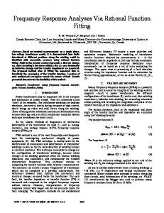
w(x) = 1 ? kex + o(ex ); x ! 1; where  < 0 is the largest negative real root of the denominator of (35) and plays a key role in the performance of the queueing system. We now compare the asymptotic decay rates obtained via the Pade approximations and the Erlang distributions with the numerical values of  we have obtained through root nding algorithms. Rather than presenting the approach as an approximation for determining the asymptotic decay rate which can easily be computed using standard numerical techniques, our aim is to show the performances of various related approximations in terms of one important parameter of the queueing system. The k-stage Erlang distributions and Pade approximations are used to approximate the asymptotic decay rate in an M/D/1 queue and the performance results of these approximations are presented in Figure 1 with respect to the utilization in the system. The notation E (k) is used to denote when the k-stage Erlang distribution is imposed. Similarly, we use the notation P (n; l) to denote the case of a Pade approximation P^n;l (s). Throughout the examples we only focus on the Pade approximations of the type P (l; l) since it is clear that P (l ? l ; l) (l > 0) and P (l; l) yield the same computational load whereas the former can match fewer moments than the latter and is not considered here. As far as the results in Figure 1 are concerned, there is a key observation, the rate of convergence (as l ! 1) of the Pade approximations to the exact asymptotic decay rate is fast whereas this convergence rate in the case of k-stage Erlang approximations is rather slow. Besides, for heavy loads ( > 0:5), the simple P (2; 2) works as well as higher order Pade approximations which makes it well-suited for use in the ATM environment due to its simplicity. However, there is the drawback of using approximations which 0

0

19

5 4.5 4

asymptotic decay rate

3.5

exact P(1,1) P(2,2) P(3,3) P(4,4) E(1) E(16)

3 2.5 2 1.5 1 0.5 0

0.1

0.2

0.3

0.4

0.5 utilization

0.6

0.7

0.8

0.9

Figure 1: Asymptotic decay rate for the M/D/1 queue. are not themselves probability distributions which is demonstrated by the break in the P (2; 2) curve at  = 0:25 which indicates there is no largest negative real root below that utilization. This is problematic (e.g., negative probabilities may result) but we recommend the use of higher order Pade approximations in the light load case for which we have not observed any such brake for the range  > 0:05. In terms of the asymptotic decay rate of the un nished work distribution, the Pade approximations work better than the Erlang approximations in the sense that to get the same degree of accuracy a signi cantly higher degree Erlang distribution is needed. This statement is also true for the general MAP/D/1/K queue as will be demonstrated by the following examples. Figure 2 is devoted to the cell loss rate approximations with respect to the buer size 20

(in cells) in an M/D/1/K queue.

cell loss rate

a) rho=0.3

P(1,1) P(2,2) P(3,3) E(1) E(4)

-5

10

cell loss rate

1

2

-5

2

cell loss rate

4 buffer size b) rho=0.6

5

6

7

6

8 buffer size c) rho=0.9

10

12

14

P(1,1) P(2,2) P(3,3) E(1) E(4)

10

4

P(1,1) P(2,2) P(3,3) E(1) E(4)

-5

10

5

3

10

15

20

25

30 35 buffer size

40

45

50

55

Figure 2: Cell loss rate approximations for the M/D/1/K queue with a)  = 0:3, b)  = 0:6, and c)  = 0:9, ( * denotes the simulation results). Three dierent cases are examined with  being 0:3, 0:6, and 0:9, respectively. P (3; 3) captures the simulation curve for all the cases whereas P (2; 2) though being indistinguishable from P (3; 3) in the latter two cases, exhibits a slight deviation in the  = 0:3 case. Even the simplest P (1; 1) works better than the E (4) for all the cases whereas its performance for the heavy load case (e.g.,  = 0:9) is quite satisfactory. Here, we recall that the key parameter that determines the computational load is the denominator degree d de ned in (9) which is k + 1 for a k-stage Erlang distribution approximation and l + 1 for the Pade approximation P^l;l(s). 21

We present our results for the MMPP/D/1/K queue in Figure 3. The input arrival process is assumed to be a superposition of N identical and independent 2-state IPP sources (users). In the silence state, the source generates no trac whereas in the activity state arrivals occur according to a Poisson process with rate P . The silence and the activity times are exponentially distributed with parameters  and , respectively. The cell loss rates based on two Pade approximants (P (1; 1) and P (2; 2)) for the case of

? = 4363:63; ? = 436:36; P = 0:275 1

1

are plotted in Figure 3 with respect to the buer size for three dierent utilizations. 0

10

-1

10

rho=0.6 P(1,1)

cell loss rate

-2

P(2,2)

10

simulation

-3

10

rho=0.2

-4

10

rho=0.1 -5

10

5

10

15

20 buffer size

25

30

35

Figure 3: Cell loss rate approximations for the MMPP/D/1/K queue with individual source parameters ? = 4363:63, ? = 436:36, and P = 0:275 and with three dierent utilizations. 1

1

Note that with the parameters above  = 0:025 N where N is the number of sources. We observe that P (2; 2) captures the simulation curve for the three trac regimes accurately 22

irrespective of the buer size. P (1; 1) overestimates the cell loss rate for small buer sizes and underestimates that for large buer sizes but it is still convenient for use for applications that can tolerate a small amount of error in accuracy with the advantage of requiring less computation. We have omitted the P (l; l) approximations with l > 2 in the gure due to the fact that they are almost identical to the P (2; 2) curve. We then x the buer size to K = 8 in the next example and assess the performance of the approximations with respect to the number of users in Figure 4. 0

10

-1

10

-2

10

cell loss rate

B=436.36 -3

10

B=4.36 -4

10

P(1,1) P(2,2)

-5

10

simulation K=8

-6

10

-7

10

5

10

15 number of users

20

25

30

Figure 4: Cell loss rate approximations for the MMPP/D/1/K queue for a small buer size, K = 8, with two dierent burst lengths of the individual source. Two sources are treated, the source of the previous example with the burst length B = 436:36 and this source with the mean activity and silence times changed to 1/100 of the previous source (B = 4:3636 in this case). While P (2; 2) gives accurate results as in the previous examples irrespective of the burst length and the load, we observe an overestimation of P (1; 1) for small loads and a slight underestimation for moderate to 23

heavy trac. The nal example attempts to demonstrate the performance of the approximations for large buer sizes. We x K = 1024 and we let each individual source (modeled as an IPP) to have the following parameters:

? = 780; ? = 20; P = 4: 1

1

Note that each source introduces a 10% load. The results are given in Figure 5 where the cell loss rate is plotted with respect to the number of users. -1

10

P=8

-2

10

-3

cell loss rate

10

P=4 -4

10

P(1,1) P(2,2)

-5

10

simulation K=1024 -6

10

-7

10

1

2

3

4

5 6 number of users

7

8

9

Figure 5: Cell loss rate approximations for the MMPP/D/1/K queue for a large buer size, K = 1024, with two dierent user peak rates. We also change the peak rate of the individual user P to 8 as well as change the mean silence time of the individual user to 1580 and present the associated results. The observation is that for the case of large buers, both two approximations P (1; 1) and P (2; 2) capture the simulation curve accurately regardless of the load. 24

References [1] J. Abate, G. L. Choudhury, and W. Whitt. Asymptotics for steady-state tail probabilities in structured Markov queueing models. Stochastic Models, 10(1), 1994. [2] J. Abate and W. Whitt. The Fourier-series method of inverting transforms of probability distributions. Queueing Systems, 10:5{88, 1992. [3] J. Abate and W. Whitt. Numerical inversion of Laplace transforms of probability distributions. ORSA journal on computing, 7(1):36{43, 1995. [4] N. Akar. Performance Analysis of an Asynchronous Transfer Mode Multiplexer with Markov Modulated Inputs. PhD thesis, Bilkent University, Ankara, Turkey, 1994. [5] N. Akar and E. Arkan. Pade approximations in the analysis of the MMPP/D/1 system. In Proc. ITC Spon. Sem., pages 137{143, Bangalore, 1993. [6] N. Akar and K. Sohraby. An invariant subspace approach in M/G/1 and G/M/1 type Markov chains. submitted to Commun. Stat.-Stochastic Models, 1995. [7] N. Akar and K. Sohraby. On computational aspects of the invariant subspace approach to teletrac problems and comparisons. submitted to Commun. Stat.Stochastic Models, 1995. [8] D. Anick, D. Mitra, and M. M. Sondhi. Stochastic theory of a data handling system with multiple sources. Bell Syst. Tech. Jour., 61:1871{1894, 1982. [9] S. Asmussen and G. Koole. Marked point processes as limits of Markovian arrival streams. J. Appl. Prob., 30:365{372, 1993. [10] A. Baiocchi. Analysis of the loss probability of the MAP/G/1/K queue Part I: Asymptotic theory. Commun. Statist. - Stochastic Models, 10(4):867{893, 1994. [11] A. Baiocchi and N. Blefari-Melazzi. Analysis of the loss probability of the MAP/G/1/K queue Part II: Approximations and numerical results. Commun. Statist. - Stochastic Models, 10(4):895{925, 1994. [12] C. Blondia. The N/G/1 nite capacity queue. Commun. Statist. - Stochastic Models, 5(2):273{294, 1989. 25

[13] C. T. Chen. Linear System Theory and Design. Holt, Rinehart and Winston, Inc., New York, 1984. [14] G. L. Choudhury, D. M. Lucantoni, and W. Whitt. Squeezing the most out of ATM. to appear in IEEE Trans. Commun., 1995. [15] A. I. Elwalid and D. Mitra. Fluid models for the analysis and design of statistical multiplexing with loss priorities on multiple classes of bursty trac. In INFOCOM'92, pages 415{425, 1992. [16] A. I. Elwalid and D. Mitra. Eective bandwidth of general Markovian trac sources and admission control of high speed networks. IEEE/ACM Trans. Netw., 1(3):329{ 343, 1993. [17] G. H. Golub and C. F. Van Loan. Matrix Computations. The Johns Hopkins University Press, Baltimore, 1989. [18] L. Gun. Experimental techniques on matrix-analytical solution techniques - extensions and comparisons. Commun. Statist. - Stochastic Models, 5(4):669{682, 1989. [19] H. Hees and D. M. Lucantoni. A Markov modulated characterization of packetized voice and data trac and related statistical multiplexer performance. IEEE JSAC, 4(6):856{868, 1986. [20] I. Ide. Superposition of interrupted Poisson processes and its application to packetized voice multiplexers. In Proc. ITC-12, 1988. [21] T. Kailath. Linear Systems. Prentice-Hall Inc., Englewood Clis NJ, 1980. [22] L. Kleinrock. Queueing Systems Volume 1: Theory. Wiley-Interscience Publication, 1975. [23] A. Kuczura. The interrupted Poisson process as an over ow process. Bell Syst. Tech. Jour., 52(3):437{448, 1973. [24] G. Latouche and V. Ramaswami. A logarithmic reduction algorithm for quasi-birthdeath processes. J. Appl. Prob., 30:650{674, 1993. [25] D. M. Lucantoni. New results for the single server queue with a batch Markovian arrival process. Stoch. Mod., 7:1{46, 1991. 26

[26] D. M. Lucantoni, G. L. Choudhury, and W. Whitt. The transient BMAP/G/1 queue. Commun. Statist. - Stochastic Models, 10(1):145{182, 1994. [27] D. M. Lucantoni, K. S. Meier-Hellstern, and M. F. Neuts. A single-server queue with server vacations and a class of non-renewal arrival processes. Adv. Appl. Prob., 22:676{705, 1990. [28] C. B. Moler and C. Van Loan. Nineteen dubious ways to compute the matrix exponential. SIAM Rev., 20:801{836, 1978. [29] M. F. Neuts. A versatile Markovian point process. J. Appl. Prob., 16:764{779, 1979. [30] M. F. Neuts. Matrix-geometric Solutions in Stochastic Models. Johns Hopkins University Press, Baltimore, MD, 1981. [31] V. Ramaswami. The N/G/1 queue and its detailed analysis. Adv. Appl. Prob., 12:222{261, 1980. [32] V. Ramaswami. Nonlinear matrix equations in applied probability - solution techniques and open problems. SIAM Review, 30(2):256{263, 1988. [33] H. Saito, M. Kawarasaki, and H. Yamada. An analysis of statistical multiplexing in an ATM transport network. IEEE JSAC, 9(3):359{367, 1991. [34] P. Skelly, M. Schwartz, and S. Dixit. A histogram-based model for video trac behavior in an ATM multiplexer. IEEE/ACM Trans. Netw., 1(4):446{459, 1993. [35] T. E. Stern and A. I. Elwalid. Analysis of separable Markov-modulated rate models for information-handling systems. Adv. Appl. Prob., 23:105{139, 1991. [36] R. C. F. Tucker. Accurate method for analysis of a packet-speech multiplexer with limited delay. IEEE Trans. Commun., 36(4):479{483, 1988. [37] J. Vlach and K. Singhal. Computer Methods for Circuit Analysis and Design. Van Nostrand Reinhold Company, New York, 1983. [38] W. Whitt. Tail probabilities with statistical multiplexing and eective bandwidths for multi-class queues. Telecommun. Syst., 2:71{107, 1993. [39] R. W. Wol. Stochastic Modeling and the Theory of Queues. Prentice Hall, Englewood Clis, NJ, 1989. 27

[40] W. M. Wonham. Linear Multivariable Control: A Geometric Approach. Springer, New York, 1974. [41] J. Ye and S. Q. Li. Analysis of multi-media trac queues with nite buer and overload control- Part I: Algorithm. In Proc. IEEE INFOCOM, pages 1464{1474, 1991. [42] J. Ye and S. Q. Li. Analysis of multi-media trac queues with nite buer and overload control- Part II: Applications. In Proc. IEEE INFOCOM, pages 848{859, 1992.

28