Kernel-Based Feature Extraction with a Speech Technology Application

2250

IEEE TRANSACTIONS ON SIGNAL PROCESSING, VOL. 52, NO. 8, AUGUST 2004

Kernel-Based Feature Extraction with a Speech Technology Application András Kocsor and László Tóth, Associate Member, IEEE

Abstract—Kernel-based nonlinear feature extraction and classification algorithms are a popular new research direction in machine learning. This paper examines their applicability to the classification of phonemes in a phonological awareness drilling software package. We first give a concise overview of the nonlinear feature extraction methods such as kernel principal component analysis (KPCA), kernel independent component analysis (KICA), kernel linear discriminant analysis (KLDA), and kernel springy discriminant analysis (KSDA). The overview deals with all the methods in a unified framework, regardless of whether they are unsupervised or supervised. The effect of the transformations on a subsequent classification is tested in combination with learning algorithms such as Gaussian mixture modeling (GMM), artificial neural nets (ANN), projection pursuit learning (PPL), decision tree-based classification (C4.5), and support vector machines (SVMs). We found, in most cases, that the transformations have a beneficial effect on the classification performance. Furthermore, the nonlinear supervised algorithms yielded the best results. Index Terms—Discriminant analysis, independent component analysis, kernel-based feature extraction, kernel-based methods, kernel feature spaces, principal component analysis.

I. INTRODUCTION

A

UTOMATIC speech recognition is dealt with by quite traditional statistical modeling techniques such as Gaussian mixture modeling or artificial neural nets. In the last couple of years, however, the theory of machine learning has developed a wide variety of novel learning and classification algorithms. In particular, the so-called kernel-based methods have recently become a flourishing new research direction. Kernel-based classification and regression techniques, including the well-known support vector machines (SVM), found their way into speech recognition relatively slowly. This is probably because their application to such large-scale tasks as speech recognition required addressing both theoretical and practical problems. Recently, however, more and more authors are turning their attention to the application of SVM in speech recognition (see, e.g., [10], [17], [46], and [50]). Besides using kernel-based classifiers, an alternative option is to use kernel-based technologies only to transform the feature space and leave the job of classification to more traditional methods [39]. The goal of this paper is to study the applicability of some of these methods to phoneme classification, making Manuscript received January 7, 2003; revised January 2, 2004. The associate editor coordinating the review of this manuscript and approving it for publication was Dr. Chin-Hui Lee. The authors are with the Research Group on Artificial Intelligence, Hungarian Academy of Sciences and University of Szeged, H-6720 Szeged, Hungary (e-mail: [email protected]; [email protected]). Digital Object Identifier 10.1109/TSP.2004.830995

use of kernel-based feature extraction methods applied prior to learning in order to improve classification rates. In essence, this paper deals with kernel principal component analysis (KPCA) [47], kernel independent component analysis (KICA) [3], [35], kernel linear discriminant analysis (KLDA) [5], [34], [40], and kernel springy discriminant analysis (KSDA) [36] techniques. Their effect on classification performance is then tested in combination with classifiers such as Gaussian mixture modeling (GMM), artificial neural networks (ANNs), projection pursuit learning (PPL), decision tree-based classification (C4.5), and support vector machines (SVMs). The algorithms are applied to two recognition tasks. One of them is real-time phoneme recognition that, when combined with a real-time visualization of the results, forms the basis of the “SpeechMaster” phonological awareness drilling software developed by our team. The other test set was the well-known TIMIT phone classification task. The structure of the paper is as follows. First, we provide a concise overview of the nonlinear feature extraction methods. The overview is written so that it deals with all the methods in a unified framework, regardless of whether they are unsupervised or supervised. Furthermore, the traditional linear counterparts of the methods can be obtained as special cases of our approach. Afterwards, we present the goals of the “SpeechMaster” software along with the phoneme classification problem that arises. Besides the special vowel-recognition task on which the “SpeechMaster” software is built, we also present test results on the TIMIT database. In both cases, we first briefly describe the acoustic features that were applied in the experiments and also list the learning methods used. Then, in the final part of the paper, we present the results of the experiments and discuss them from several aspects, focusing on the advantages and drawbacks of each nonlinear feature extraction method. II. KERNEL-BASED FEATURE EXTRACTION Classification algorithms require that the objects to be classified are represented as points in a multidimensional feature space. However, before executing a learning algorithm, additional vector space transformations may be applied on the initial features. The reason for doing this is twofold. First, they can improve classification performance, and second, they can reduce the dimensionality of the data. In the literature, sometimes both the choice of the initial features and their transformation are dealt with under the name “feature extraction.” To avoid any misunderstanding, in this section, it will cover only the latter, that is, the transformation of the initial feature set into another one, which is hoped will yield a more efficient or, at least, faster classification.

1053-587X/04$20.00 © 2004 IEEE

KOCSOR AND TÓTH: KERNEL-BASED FEATURE EXTRACTION WITH A SPEECH TECHNOLOGY APPLICATION

The approach of feature extraction could be either linear or nonlinear, but there is a technique (which is most topical nowadays) that is, in some sense, breaking down the barrier between the two types. The key idea behind the kernel technique was originally presented in [1] and was again applied in connection with the general purpose SVM [8], [11], [49], [52], [53], which was later followed by other kernel-based methods [3], [5], [34], [35], [40], [45], [47], [48]. In the following, we summarize four nonlinear feature extraction methods that may be derived using the kernel-based nonlinearizations of the linear algorithms PCA, ICA, LDA, and SDA. We do not present the linear techniques separately because the nonlinear descriptions will be formalized in such a way that, with a proper parametrization, they lead back to the traditional linear methods. All methods will be dealt with in a unified, concise form. We also represent the effects of these transformations on artificial data sets via figures. In addition, we always give references to sources where a detailed description on the feature extraction technique in question can be found. Our main aim is to help the reader gain a unified view of the methods and get some ideas about their usage. First, we provide a set of definitions. Then, we discuss the kernel idea, followed by an explanation of each method one after the other. The section ends with some remarks about how the number of required calculations can be reduced by decimating the sample set. A. Introduction Without loss of generality, we will assume that as a realization of multivariate random variables, there are -dimensional real attribute vectors in a compact set over describing objects sample matrix in a certain domain and that we have a finite containing random observations. Let us also assume that we have classes and an indicator function (1) where gives the class label of the sample . Let further denote the number of vectors associated with label in the sample data.1 Now, we continue with the definition of the kernel-based feature extraction and then outline the kernel idea. The goal of feature extraction is to find a mapping , which leads to a new set of features that are optimal according to a given criterion. In the case of kernel-based feature extraction, the mapping is nonlinear and has the following form: (2) where

is a constant, real matrix, the function is continuous, symmetric and positive definite (which is called a Mercer kernel), is the sample matrix, and is a short-hand notation for the vector . As can be seen in (2), linear combinations of the base functions give the components of the new feature . The criterion [and hence the calculation that leads vector to matrix in (2)] is different for each method, and the result depends on the data set . 1The two types of feature extraction methods (supervised or unsupervised) can be distinguished by whether they utilize an indicator function or not during the computation of the transformation parameters.

2251

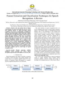
Fig. 1. ”Kernel-idea.” The dot product in the kernel feature space F is defined implicitly.

Based on Mercer’s theorem [53], if is a Mercer kernel, then a dot product space necessarily exists with a mapping (see Fig. 1) such that (3) Usually, is called the kernel feature space, and is the feature map. At this point, we have two immediate consequences. When is the identity, the function (the simple dot product over the space ) is symmetric, continuous, and positive definite; therefore, it constitutes a proper Mercer kernel. Going the other way, when applying a general Mercer kernel, we can assume a space over which we perform dot product calculations. This space and dot product calculations over it are defined only implicitly via the kernel function itself. The space and map may not be explicitly known. We need only define the kernel function, which then ensures an implicit evaluation. The construction of Mercer kernels, when such a mapping exists, is a nontrivial problem, but there are some possible candidates available (cf. [13], [18], [32]). From the functions available, the three most popular are the polynomial kernel , the Gaussian RBF kernel , and the rational quadratic kernel :

(4) Let us suppose that we have chosen a specific kernel function along with a proper feature map and a kernel feature space . Then, the nonlinear mapping of (2) can be written as .. .

.. . In the following, we will denote the latter matrix by . Notice here that is constant, and its rows contain linear combinations

2252

IEEE TRANSACTIONS ON SIGNAL PROCESSING, VOL. 52, NO. 8, AUGUST 2004

of the image of the data vectors in . This means that the transformation is linear in the kernel feature space, but because the feature map itself is nonlinear, we obtain a nonlinear transformation of the sample points of the initial feature space . All the algorithms that we are going to present in the following are linear mappings in the kernel feature space, the row vectors of matrix being obtained by optimizing a different objective function , say. What is common in each case is that we will look for directions with large values of . Intuitively, if larger values of indicate better directions and the row vectors of need to be independent in certain ways, choosing stationary largest function values is a reasonable points that have the strategy. Obtaining the above stationary points of a general objective function is a difficult global optimization problem, but if is defined by a Rayleigh quotient formula

We can arrive at this assumption in many ways, e.g., we can into vectors , decompose an arbitrary vector gives that component of , which falls in where , whereas gives the compoand nent perpendicular to it. Since for the stationary points the eigenvalue-eigenvector equality is satisfied, we find that the condition defined in (9) ) does not restrict generality. (i.e., Based on the above assumption the variational parameters of can be the vector instead of

(5) the solution is easy and fast when formulated as a generalized eigenvalue problem . Actually, this approach offers a unified view of the feature extraction methods discussed in this paper. B. Kernel Principal Component Analysis Principal component analysis (PCA) [29] is a ubiquitous unsupervised technique for data analysis and dimension reduction. To explain how its nonlinear version works [47], 2 let us first choose a kernel function for which

(10)

It is easy to see that (11) where is a Gram matrix, is the unit matrix, and . After differentiating (11) with respect to , we find that the stationary points are the solution vectors of the general eigenvalue problem (12) which is equivalent to the problem (13)

holds for a mapping . It is well-known that PCA looks for those directions of in which the variance of the data is large. We will do exactly the same but in the kernel feature space . For this, we define the objective function as (6) where

is not symmetric, its eigenvalues Although the matrix are real and non-negative, and those eigenvectors that have positive eigenvalues are orthogonal. In fact, the best approach is to solve the following symmetric eigenproblem, where the positive eigenvalues and the corresponding eigenvectors are the same as those obtained from (13)

is the covariance matrix of the image of the sample : (7)

Now, we define the Kernel-PCA transformation based on the stationary points of (6), which are given as the eigenvectors of the symmetric positive semidefinite matrix . However, since this matrix is of the form (8) we can suppose the following equation holds during the analysis of the stationary points: (9) 2The derivation presented here differs slightly from the one originally proposed by Schölkopf, but the result of the derivation is equivalent to the original.

(14) positive dominant eigenvalues of be denoted by and the corre. Then, the matrix of sponding eigenvectors be the transformation we need (cf. (2)) can be calculated like Now, let the

(15) The effect of KPCA is demonstrated in Fig. 2. The data set of Fig. 2(a) was transformed using linear PCA, that is, KPCA . The result is was performed using the kernel shown in Fig. 2(b). Evidently, the algorithm found the direction with the largest variance and chose it as the -axis of the transformed data. This effect is also justified by the shape of distribution curves shown below the images. In a second experiment the data set of Fig. 2(d) was transformed but, in this case, using the rational quadratic kernel, which leads to a nonlinear transformation. The result is shown in Fig. 2(e). Examining the distribution of the points along the -axis, one can see that the variance of

KOCSOR AND TÓTH: KERNEL-BASED FEATURE EXTRACTION WITH A SPEECH TECHNOLOGY APPLICATION

2253

Fig. 2. Typical behavior of KPCA and KICA. (a) and (d) show some artificial data sets before the transformation. (b) and (e) show the resulting distribution after linear and nonlinear KPCA, respectively. (c) and (f) depict the results of a linear and nonlinear KICA. The distribution of the data points along the x-axis is shown below each figure.

the data has significantly increased owing to the nonlinearity of the method employed. C. Kernel Independent Component Analysis Independent component analysis [12], [15], [26]–[28] (ICA) is a general-purpose statistical method that originally arose from the study of blind source separation (BSS). Another application of ICA is unsupervised feature extraction, where the aim is to linearly transform the input data into uncorrelated components, along which the distribution of the sample set is the least Gaussian. The reason for this is that along these directions, the data is supposedly easier to classify. This is in concordance with the most common speech modeling technique, that is, fitting mixtures of Gaussians on each class. Obviously, this assumes that the class distributions can be well approximated by Gaussian mixtures. ICA extends this by assuming that the distribution when all classes are fused, on the contrary, is not Gaussian; therefore, using non-Gaussianity as a heuristic for unsupervised feature extraction will prefer those directions that separate the classes. For optimal selection of the independent directions, several objective functions were defined using approximately equivalent approaches. The goal of the ICA algorithm itself is to find the optimum of these objective functions. There are many itera-

tive methods for performing ICA. Some of these require preprocessing, i.e., centering and whitening, whereas others do not. In general, experience shows that all these algorithms should converge faster on centered and whitened data, even with those that do not really require it. Let us first examine how the centering and whitening preprocessing steps can be performed in the kernel feature space. To this end, let the inner product be implicitly defined by the kernel function in with associated transformation . Centering in . We shift the data with its to obtain data mean .. . (16) with a mean of . Whitening in . The goal of this step is to transform the cenvia an orthogonal transformatered samples tion into vectors , where the covariance matrix is the unit matrix. Since standard PCA [29]—just like its kernel-based counterpart—transforms the covariance matrix into a diagonal form, where the diagonal elements are the eigenvalues of the

2254

IEEE TRANSACTIONS ON SIGNAL PROCESSING, VOL. 52, NO. 8, AUGUST 2004

data covariance matrix , it only remains to transform each diagonal element to 1. Based on this observation, the required whitening transformation is obtained by slightly modifying the formulas presented in the section on KPCA. are Now, if we assume that the eigenpairs of and , the transformation matrix will take the form . If is less than , a dimensionality reduction is employed. After the nonlinear preprocessing, we can apply one of the many linear ICA algorithms. We present here the FastICA algorithm of Hyvärinen, for which centralization and whitening is a prerequisite. For the sake of simplicity, here, we will denote the prepro. In this new linear space, we cessed data samples by are going to search for directions along which the distribution of the data is the least Gaussian. To measure this criterion, we introduce the following objective function: (17) where is a variable with zero mean and unit variance, is an appropriate nonquadratic function, again denotes the expectation value, and is a standardized Gaussian variable. The following three choices of are conventionally used:

(18) It should be mentioned here that in (17), the expectation value of is a constant, its value only depending on the selected ). The variable has a leptokurtic function (e.g., distribution (a distribution with a high peak) if , it is a mesokurtic variable if , whereas it has platykurtic distribution (i.e., it is a flat-topped curve) when . For leptokurtic independent components, the optimal contrast function is one that grows slower than quadratically, whereas the optimal for platykurtic components grows faster (cf. [28]). In Hyvärinen’s FastICA algorithm for selecting a new direction , the following objective function is used: (19) , the dot which may be obtained by replacing in (17) with product of the direction , and sample . FastICA is an approximate Newton iteration procedure for the local optimization of . the function Before discussing the optimization problem, let us first examine the properties of the preprocessed data . a) For every normalized vector the mean of is set to zero, and its variance is set to one. Actually, we need this since (17) requires that should have a zero mean and variance of one; hence, , the projected data with the substitution must also have this property.

of the transb) For any matrix , the covariance matrix will remain formed preprocessed points is orthogonal since a unit matrix if and only if

(20) After preprocessing, FastICA looks for a new orthogonal base for the preprocessed data, where the values of the non-Gausfor the base vectors are large. Note that since sianity measure the data remains whitened after an orthogonal transformation, ICA can be considered an extension of PCA. Now, we briefly outline how the FastICA algorithm works (cf. [15], [27]). The input for this algorithm is the preprocessed and the nonlinear function , sample whereas the output is the transformation matrix . The firstand . and second-order derivatives of are denoted by procedure FastICA ; % initialization be a random matrix; let ; ; % approximate Newton iteration has not converged; While to for let be the th raw vector of ; end; ; ; ; do End procedure

;

means a symmetric In the pseudo-code, decorrelation, where can be readily obtained from its eigenvalue decomposition. If , then is equal to . Finally, the expected values required by the algorithm are calculated as the empirical means of the preprocessed input samples in . We should remark that in the discussion above, we nonlinearized only centering and whitening and not the consecutive iterative FastICA algorithm. It would also be possible, as in , that the dot product could be nonlinearized with the kernel method, but this would go outside our unified discussion based on the Rayleigh quotient. Practically speaking, the Kernel FastICA method Kernel-Centering Kernel-Whitening iterative process of the original FastICA. The transformation ma, where represents centering trix (cf. (2)) of KICA is and whitening, whereas corresponds to the orthogonal matrix produced by FastICA. Despite the fact that the second, optimizais not based on the Rayleigh quotient tion phase for finding approach, we feel that KICA, as a unique extension of KPCA, can be the part of this review. More details on the family of the KICA methods can be found in [3] and [34].

KOCSOR AND TÓTH: KERNEL-BASED FEATURE EXTRACTION WITH A SPEECH TECHNOLOGY APPLICATION

To demonstrate the behavior of KICA, we return to the artificial data set in Fig. 2. We once again transformed the data sets (a) and (a) but now with KICA. Fig. 2(c) shows the result when using a linear kernel, whereas Fig. 2(f) shows the effect of a rational quadratic kernel. When compared with KPCA, it can be readily seen that although KPCA looks for directions with a large variance, KICA prefers those directions with the least possible Gaussian distribution.

2255

We may also suppose without loss of generality here that holds during the search for the stationary points of (21). With this assumption, after some algebraic rearrangement, we obtain the formula (24) where

is the kernel matrix,

, and

D. Kernel Linear Discriminant Analysis Linear discriminant analysis (LDA) is a traditional supervised feature extraction method [16] that has proved to be one of the most successful preprocessing techniques for classification. It has long been used in speech recognition as well [4], [22], [51]. The goal of LDA is to find a new (not necessarily orthogonal) basis for the data that provides the optimal separation between classes. To present the steps of KLDA, we virtually follow the discussion of its linear counterpart, but in this case, everything is meant to happen implicitly in the kernel feature space . Let us again suppose that a kernel function has been chosen along with a feature map and a kernel feature space . In order to define the transformation matrix of KLDA, we first define , which depends not only on the objective function the sample data but also on the indicator function owing to the supervised nature of this method. Let us define (21) where is the between-class scatter matrix, whereas is the within-class scatter matrix. Here, the between-class scatter matrix shows the scatter of the class mean vectors around the overall mean vector :

if otherwise.

(25)

This means that (21) can be expressed as dot products and that the stationary points of this of equation can be computed using the real eigenvectors of . Since, in general, is a positive semidefinite matrix, it can be forced to be invertible if we add a small positive constant to its diagonal, that is, we work with instead of . This matrix is guaranteed to be positive definite and, hence, should always be invertible. This small act of cheating can have only a negligible effect on the stationary points of (21). If we further assume that the real eigenvalues of real eigenvectors with the largest are , then the transformation matrix (cf. (2)) will be . The behavior of KLDA is illustrated in Fig. 3 in the two examples of (a) and (d). In both cases, the application of the exponential kernel resulted in a nonlinear transformation that minimized the variance of the classes while giving the best spatial class separation at the same time. The results are shown in Fig. 3(b) and (e), respectively. Noting the distribution of the classes along the -axis, one can see that their separability has increased. E. Kernel Springy Discriminant Analysis

(22) The within-class scatter matrix represents the weighted average scatter of the covariance matrices of the sample vectors with the class label :

As was shown in Section II-D, the KLDA criterion leads to a nonsymmetric matrix, the eigenvectors of which are not necessarily orthogonal. Furthermore, we had to apply the shifting of the eigenspectrum to avoid numerical complications during inversion. These issues give rise to the need for an objective function , which results in a supervised transformation and yields similar results to KLDA but is orthogonal and avoids the numerical problems mentioned. Now, let the dot product be implicitly defined (see Fig. 1) by the kernel function in the kernel feature space with associated transformation : (26)

(23) is large when its nominator is large and its denominator is small or, equivalently, when in the kernel feature space , the within-class averages of the sample projected onto are far from each other, and the variance of the classes is small. The , the farther the classes will be spaced, larger the value of and the smaller their spreads will be.

The name kernel springy discriminant analysis stems from the utilization of a spring and antispring model, which involves searching for directions with optimal potential energy using attractive and repulsive forces. In our case, sample pairs in each class are connected by springs, whereas those of different classes are connected by antisprings. New features can be easily extracted by taking the projection of a new point in those directions having a small spread in each class, while different , which is classes are spaced out as much as possible. Let

2256

IEEE TRANSACTIONS ON SIGNAL PROCESSING, VOL. 52, NO. 8, AUGUST 2004

Fig. 3. Effect of the supervised algorithms KLDA and KSDA. (a) and (d) depict artificial data sets. (b) and (e) show the resulting data sets after applying KLDA on (a) and (d), respectively. (c) and (f) represent the KSDA-transformed versions of (a) and (d). The distributions of the classes along the x-axis is also shown below the figures. In every case, the transformation applied was nonlinear.

the potential of the spring model along the direction defined by

in

, be

It is easy to prove that quotient formula:

is equal to the following Rayleigh

(31)

(27) where where

(32) if otherwise

(28)

Naturally, the elements of matrix can be initialized with values different from as well. Each element of the matrix can be considered as a kind of spring quotient, and each can be set to a different value for any pair of data points. As before, we again suppose that the directions can be constructed as the linear combinations of the images of the data points in . That is (29) . To find the directions with where large potentials, let the objective function be defined by (30)

Moreover, it is also straightforward to prove that (31) takes the following form: (33) where is again the kernel matrix, and is a diagonal matrix with the sum of each row of in the diagonal. After taking the derivative of (33), it is readily seen that the stationary points can be obtained via an eigenanalysis of the following of symmetric eigenproblem: (34) , If we assume that the dominant eigenvectors are then the transformation matrix in (2) is defined by .

KOCSOR AND TÓTH: KERNEL-BASED FEATURE EXTRACTION WITH A SPEECH TECHNOLOGY APPLICATION

The effect of KSDA can again be visualized by transforming the data sets of Fig. 3(a) and (d). While KLDA aims at minimizing the within-class variance and maximizing the between-class distance, KSDA does something similar but based on within-class attractive and between-class repulsive forces. The results presented in Fig. 3(c) and (f) have a clearly separable class structure like those obtained using KLDA.

2257

representation). Obviously, as in practice, the feature space is of lower dimension, and it is worth using the linear methods when the simple dot product kernel is chosen. Now, we show that the nonlinear formulae obtained by this kernel function are readily traced back to the linear ones. Let us notice that in this case, the ; thus kernel matrix is equal to PCA ICA

F. Reducing the Computational Cost As we have already seen, all four methods lead to a (generalized) eigenproblem that involves finding the stationary points of the objective function that is defined in the form of a Rayleigh quotient. During optimalization, the vector consists of the linear combinations of the images of the data points in the kernel feature space. Without doubt, if the amount is large, then the -sized matrices that of data points —hence for solving the eigenare needed for constructing problem—can be so big that they pose serious computational and memory management problems. Fortunately, in most practical problems, good directions data points instead can be found even if we use only of when constructing the linear combinations. Let us denote . It is the indices of these samples by easy to check that by just using these data items, the formulas we can be expressed by the following: obtain for the function KPCA KICA

(35)

KLDA

(36)

KSDA

(37)

is the matrix constructed where is a vector of dimension , of the kernel matrix , and is from the columns the minor matrix determined by the rows and columns of with . Based on these formulas, the eigenproblems indices to be solved are now reduced to a matrix of size . In practice, this matrix usually has no more than a couple of dozen or a couple of hundred rows and columns. Of course, a key issue here is the strategy for choosing the indices. Numerous selection strategies are possible from the random selection to the exhaustive search approach. In this paper, we restrict our investigations to two different selection techniques. The first one is the simplest case when we chose samples randomly, where, in the second, we employed the kernel variant of the sequential forward floating selection (SFFS [43]) method with the LDA optimization criterion [37]. One more issue occurs that we need to discuss here. It is well known that for the linear feature extraction methods PCA, ICA, LDA, and SDA, the size of the problem is that of the original feature space. However, it depends on the number of the samples in the kernel counterparts. Despite these differences, if the kernel and function is defined by the simple dot product , then the the feature map is realized by the identity kernel formulation of the methods (dual representation) are undoubtedly equivalent to the corresponding linear cases (primal

(38) LDA (39) SDA (40) where the vector , mension.

, and matrices and

, are of the lower di-

III. EXPERIMENT 1: CLASSIFICATION OF STEADY-STATE VOWELS A. Application: Phonological Awareness Teaching System The “SpeechMaster” software developed by our team seeks to apply speech recognition technology to speech therapy and the teaching of reading. The role of speech recognition is to provide a visual phonetic feedback. In the first case, it is intended to supplement the missing auditive feedback of the hearing impaired, whereas in the case of the latter, it is to reinforce the correct association between the phoneme-grapheme pairs. With the aid of a computer, children can practice without the need for the continuous presence of the teacher. This is very important because the therapy of the hearing impaired requires a long and tedious fixation phase. Furthermore, experience shows that most children prefer computer exercises to conventional drills. Both applications require a real-time response from the system in the form of an easily comprehensible visual feedback. With the simplest display setting, feedback is given by means of flickering letters, their identity and brightness being adjusted to the speech recognizer’s output. Fig. 4 shows the user interface of “SpeechMaster” in the teaching reading and the speech therapy applications, respectively. As one can see, in the first case, the flickering letter is positioned over a traditional picture for associating the word and word sound, whereas in the latter case, it is combined with a web camera image, which helps the impaired student learn the proper articulator positions. B. Evaluation Domain For training and testing purposes, we recorded samples from 160 children aged between 6 and 8. The ratio of girls and boys was 50%–50%.The speech signals were recorded and stored at a sampling rate of 22 050 Hz in 16-bit quality. Each speaker uttered all the Hungarian vowels, one after the other, separated

2258

IEEE TRANSACTIONS ON SIGNAL PROCESSING, VOL. 52, NO. 8, AUGUST 2004

Fig. 4. Screenshots of the “SpeechMaster” phonological awareness teaching system. (a) Teaching reading part. (b) Speech therapy part. TABLE I RECOGNITION ERRORS ON EACH FEATURE SET AS A FUNCTION OF THE TRANSFORMATION AND CLASSIFICATION APPLIED

by a short pause. Since we decided not to discriminate their long and short versions, we only worked with nine vowels altogether. The recordings were divided into a train and a test set in a ratio of 50%–50%. C. Acoustic Features There are numerous methods for obtaining representative feature vectors from speech data [24], but their common property is that they are all extracted from 20–30 ms chunks or “frames” of the signal in 5–10-ms time steps. The simplest possible feature set consists of the so-called bark-scaled filterbank log-energies (FBLEs). This means that the signal is decomposed with a special filterbank, and the energies in these filters are used to parameterize speech on a frame-by-frame basis. In our tests, the filters were approximated via Fourier analysis with a triangular weighting, as described in [24]. Altogether, 24 filters were necessary to cover the frequency range from 0 to 11 025 Hz. Although the resulting log-energy values are usually sent through a cosine transform to obtain the well-known mel-frequency cepstral coefficients, we abandoned it for two reasons: 1) The transforms we were going to apply have a similar decor-

relating effect, and 2) we observed earlier that the learners we work with—apart from GMM—are not sensitive to feature correlation; consequently, the cosine transform would bring no significant improvement [33]. Furthermore, as the data consisted of steady-state vowels, we found in a pilot test that adding the usual delta and delta-delta features could only marginally improve the results. Therefore, only the 24 filter bank log-energies formed this feature set, which were always extracted from the center frame of the vowels. Although it would be possible to stack several neighboring frames to form a larger feature set, because of the special steady-state nature of the vowel data used, we saw no point in doing so. The filterbank log-energies seem to be a proper feature set for a general speech recognition task as their spectro-temporal modulation is supposed to carry all the speech information [41], but in the special task of classifying vowels pronounced in isolation, it is only the gross spectral shape that carries the phonetic information. More precisely, it is known from phonetics that the spectral peaks (called formants) code the identity of vowels [41]. To estimate the formants, we implemented a simple algorithm that calculates the gravity centers and the variance of the mass in certain frequency bands [2]. The frequency bands are chosen so

KOCSOR AND TÓTH: KERNEL-BASED FEATURE EXTRACTION WITH A SPEECH TECHNOLOGY APPLICATION

that they cover the possible place of the first, second, and third formants. This resulted in six new features altogether. A more sophisticated option for the analysis of the spectral shape would be to apply some kind of auditory model [21]. Unfortunately, most of these models are too slow for a real-time application. For this reason, we experimented with the in-synchrony-bands-spectrum of Ghitza [19] because it is computationally simple and attempts to model the dominance relations of the spectral components. The model analyzes the signal using a filterbank that is approximated by weighting the output of an FFT—quite similar to the FBLE analysis. In this case, however, the output is not the total energy of the filter but the frequency of the component that has the maximal energy; therefore, it dominates the given frequency band. Obviously, the output resulting from this analysis contains no information about the energies in the filters but only about their relative dominance. Hence, we supposed that this feature set complements the FBLE features in a certain sense. D. Learners Describing the mathematical background of the learning algorithms applied is beyond the scope of this paper. Besides, we believe that they are familiar to those who are acquainted with pattern recognition. Therefore, in the following, we specify only the parameters and the training algorithms used with each learner, respectively. 1) Gaussian Mixture Modeling: The most widely used method for modeling the class-conditional (continuous) distribution of the features is to approximate it by means of a weighted sum of Gaussians [14]. Traditionally, the parameters are optimized according to the maximum likelihood (ML) criterion, using the expectation-maximization (EM) algorithm. It is well known, however, especially in the speech community, that maximum likelihood training is not optimal from a discrimination point of view as it disregards the competing classes. Several alternatives have been proposed, such as maximum mutual information (MMI) [42], [54] or minimum classification error (MCE) criteria [30], [31]. Although these alternative training methods can significantly boost the classification performance, the increased computational requirements—especially when embedded in a hidden Markov model (HMM)—seems to be a deterrent to their widespread usage. Here, we will utilize the EM algorithm with the following setup. As EM is an iterative technique, it requires a proper initialization of the parameters. To find a good starting parameter set, we applied -means clustering [16]. Since -means clustering again only guaranteed finding a local optimum, we ran it 15 times with random parameters and used the one with the highest log-likelihood to initialize the EM algorithm. After experimenting, the best value for the number of mixtures was found to be 3. In all cases, the covariance matrices were forced to be diagonal. 2) Artificial Neural Networks: Since it was realized that under proper conditions, ANNs can model the class posteriors [7], neural nets are becoming evermore popular in the speech recognition community. In the ANN experiments, we used the most common feed-forward multilayer perceptron network with the backpropagation learning rule. The number of neurons

2259

in the hidden layer was set at 18 in each experiment (this value was chosen empirically, based on preliminary experiments). Training was stopped based on the cross-validation of 15% of the training data. 3) Projection Pursuit Learning: Projection pursuit learning is a relatively little-known modeling technique. It can be viewed as a neural net where the rigid sigmoid function is replaced by an interpolating polynomial. With this modification, the representation power of the model is increased, so fewer units are necessary. Moreover, there is no need for additional hidden layers; one layer plus a second layer with linear combinations will suffice. During learning, the model looks for directions in which the projection of the data points can be well approximated by its polynomials; thus, the mean square error will have the smallest value (hence the name “projection pursuit”). Our implementation follows the paper of [25]. In each experiment, a model with eight projections and a fifth-order polynomial was applied. 4) Support Vector Machines: The SVM is a classifier algorithm that is based on the same kernel idea that we presented earlier. It first maps the data points into a high-dimensional feature space by applying some kernel function. Then, assuming that the data points have become easily separable in the kernel-space, it performs linear classifications to separate the classes. A linear hyperplane is chosen with a maximal margin. For further details on SVMs, see [53]. In all the experiments with SVMs, the radial basis kernel function was applied. E. Experimental Setup In the experiments, five feature sets were constructed from the initial acoustic features, as described in Section III-B. Set1 contained the 24 FBLE features. In Set2, we combined Set1 with the gravity center features; therefore, Set2 contained 30 measurements. Set3 was composed of the 24 SBS features, whereas in Set4, we combined the FBLE and SBS sets. Last, in Set5, we added all the FBLE, SBS, and gravity center features, thus obtaining a set of 54 values. With regard to the transformations, in every case, we kept only the first eight components. We performed this severe dimension reduction in order to show that when combined with the transformations, the classifiers can yield the same scores in spite of the reduced feature set. To study the effects of nonlinearity, the linear version of each transformation was also used on each feature set. To obtain a sparse data representation for the kernel methods, we reduced the number of data points to 200 by applying the SFFS selection technique discussed earlier. Preliminary experiments showed that using more data would have no significant effect on the results. In the classification experiments, every transformation was combined with every classifier on every feature set. This resulted in the large table of Table I. In the header of the table, PCA, ICA, LDA, and SDA stand for the linear transformations was used), whereas KPCA, KICA, KLDA, (i.e., the kernel and KSDA stand for the nonlinear transformations (with an exponential kernel), respectively. The numbers shown are the recognition errors on the test data. The number in parenthesis denotes the number of features preserved after transformation. The best scores of each set are given in bold.

2260

IEEE TRANSACTIONS ON SIGNAL PROCESSING, VOL. 52, NO. 8, AUGUST 2004

F. Results and Discussion

for testing (51681 phone instances). The phone labels were fused into 39 classes, according to [38].

Upon inspecting the results, the first thing one notices is that the SBS feature set (Set3) did about twice as badly as the other sets, no matter what transformation or classifier was tried. When combined with the FBLE features (Set1), both the gravity center and the SBS features brought some improvement, but this improvement is quite small and varies from method to method. When focusing on the performance of the classifiers, ANN, PPL, and SVM yielded very similar results. They, however, consistently outperformed GMM, which is the method most commonly used in speech technology today. First, this can be attributed to the fact that the functions that a GMM (with diagonal covariances) is able to represent are more restricted in shape than those of ANN or PPL. Second, it is a consequence of modeling the classes separately, rather than in the case of the other three classifiers, that optimize a discriminative error function. With regard to the transformations, an important observation is that after the transformations, the classification scores did not get worse compared with the classifications when no transformation was applied. This is so in spite of the dimension reduction, which shows that the features are highly redundant. Removing this redundancy by means of a transformation can make the classification more robust and, of course, faster. Comparing the linear and the kernel-based algorithms, there is a slight preference toward the supervised transformations rather than the unsupervised ones. Similarly, the nonlinear transforms yielded somewhat better scores than the linear ones. The best transformation-classifier combination, however, varies from set to set. This warns us that no such broad claim can really be made about one transformation being superior to the others. This is always dependent on the feature set and the classifier. This is, of course, in accordance with the “no free lunch” theorem, which claims that for different learning tasks, different inductive bias can be beneficial [14]. Finally, we should make some general remarks. First of all, we must emphasize that both the transformations and the classifiers have quite a few adjustable parameters, and to examine all parameter combinations is practically impossible. Changing some of these parameters can sometimes have a significant effect on the classification scores. Keeping this (and the no-freelunch theorem) in mind, our goal in this paper was to show that the nonlinear supervised transformations have the tendency to perform better (with any given classifier) than the linear and/or unsupervised methods. The results here seem to justify our hypothesis. IV. EXPERIMENT 2: TIMIT PHONE CLASSIFICATION A. Evaluation Domain In the vowel experiments, the database, the number of features, and the number of classes were all smaller than in a common speech recognition task. To assess the applicability of the algorithms to larger scale problems, we also ran phone classification tests on the TIMIT database. The train and test sentences were chosen as usual, that is, 3696 “sx” and “si” sentences formed the train set (142 909 phone instances), and the complete test set (1344 “si” and “sx” sentences) were used

B. Acoustic Features For the frame-based description of the signals, we again used the bark-scaled filterbank log-energies. Twenty two filters were applied to cover the 0–8000-Hz frequency range of the TIMIT recordings. Because the phonetic segments of the corpus are composed of a varying number of frames, an additional step was required to make them tractable for the transformations and learners, as these need all segments to be represented by the same number of features. For this, we applied the very simple strategy of dividing each segment into three thirds and averaging the filterbank energies over these subsegments (from a signal processing view this means a nonuniform smoothing and resampling). This method was popularized mainly in the SUMMIT system [20] but was also successfully applied by others as well [10]. To allow the learner to model the observation context at least to a certain level, additional average filterbank energies were calculated at the beginning and end of the segments. For this aim, 50–50 ms intervals were considered on both sides. energy-based features per Besides the resulting segment, the length of the phone was also utilized. Furthermore, similar to the usual frame-based description strategies, we found that derivative-like features can be very useful—but, in our case, extracted only at the segment boundaries. These were calculated by RASTA filtering the energy trajectories and then simply taking the frame-based differences at the boundaries. The role of RASTA filtering is to smooth the trajectories by removing those modulation frequency components that are perceptually not important [23]. In preliminary experiments, we have found that it is unnecessary to calculate these delta-features in every bark-wide frequency channel. Rather, we have concluded that it is enough to extract them from fewer but wider frequency bands (this idea was in fact motivated by physiological results on the tuning curves of cochlear nucleus onset cells). Accordingly, only four six-bark wide channels were used to calculate the delta features, altogether resulting in eight of them (4–4 at each of the boundaries). Finally, we have observed that smoothing over the segment thirds can sometimes remove important information, especially when working with long phone instances. To alleviate this, we extended our feature set with the variances of the energies calculated over the segments. These were again calculated only from the four wide bands described above. Altogether, 123 segmental features were extracted from every phone instance. To justify the correctness of our representation, we ran some preliminary classification tests, and the results were very close to those of others using a similar feature extraction technique [10], [20]. C. Learners The TIMIT data set is much bigger than our vowel database. Consequently, we had no capacity to test every combination of the classifiers and learners, as we did in the case of the vowel data. Thus, we decided to restrict ourselves to two classifiers only. ANN was chosen because of its consistently good performance and relatively small training time. The other classifier

KOCSOR AND TÓTH: KERNEL-BASED FEATURE EXTRACTION WITH A SPEECH TECHNOLOGY APPLICATION

was selected based on the following rationale. The main aim of transforming the features space is to rearrange the data points so that they become more easily modelable by the subsequent learner. In accordance with this, the transforms must bring the most improvement when applied prior to a learner with a relatively small representation power. Therefore, as the second classifier, we chose C4.5. This is a well-known classifier in machine learning, and when trained on numerical data, it has a very restricted representation technique. 1) Artificial Neural Networks: In all the experiments, the ANN had 38 inputs and 300 neurons in the hidden layer. Training was stopped based on cross-validation over 15% of the training data. 2) C4.5: C4.5 is a very well-known and widely used classifier in the machine learning community [44]. For those who prefer a statistical view, very similar learning schemes can be found under the name Classification and Regression Trees [9]. This method builds a tree-based representation from the data and was originally invented with nominal features in mind. The algorithm was, however, extended for the case of numerical features. In this case, the algorithm decomposes the feature space into rectangular blocks by means of axis-wise hyperplanes. The hypercubes are iteratively decomposed into smaller and smaller ones, according to an entropy-based tree-building rule. This hashing of the feature space can be stopped by many possible criterions. Finally, class labels are attached to each hyperbox, but posterior probability estimations are also easily attainable based on frequency counts. Obviously, the limited representation power of the model is caused both by the axis-wise restriction on the hyperplanes and the step-like look of the resulting probability estimations. In the experiments, we used the original implementation of Quinlan. During tree building, the minimum number of data points per leave was set to 24. The default parameters were used in every other respect. D. Experimental Setup Both the ANN and C4.5 classifiers were combined with each transformation. In the case of the kernel algorithms, we always used the Gaussian RBF kernel [see (4)]. The number of features extracted by the transformations was always set to 38, that is, the number of classes minus one. This value was chosen because LDA cannot return any more components (without tricks like splitting each class into subclasses), and to keep the results comparable, we used the same number of features for the other transformations as well. With regard to sparse data representation, because of the large size of the database, we could not apply the SFFS technique (as its memory requirement is a quadratic function of the database size). Therefore, we decided to select the data points randomly, starting from 100 points, and iteratively adding further sets of 100 points. This was done in order to see how the number of points affected performance. We were also interested in whether the choice of the contrast function of ICA influences its class separation abilities. To this end, to learn more about this, we performed tests with all three contrast functions listed in (18). Both linear ICA and Kernel-ICA (with an RBF kernel) were tried with all three contrast functions. The results showed that there were only small differences, but on the TIMIT data, the contrast function

2261

Fig. 5. Classification error as a function of the number of points kept in the sparse representation. TABLE II RECOGNITION ERRORS ON TIMIT

seemed to behave the best. In the rest of the test, we always worked with this contrast function. E. Results and Discussion The results of iteratively increasing the number of data points are plotted in Fig. 5. On every set, Kernel-LDA was applied, with a subsequent ANN and C4.5 learning. The diagram shows how the classification error changes when the number of data is increased with a step size of 100. Clearly, the improvement is more dramatic for the C4.5 than for the ANN. In both cases, there was no significant improvement beyond a sample size of 600. In the following experiments, we always used this set of 600 points in the kernel-based tests. The classification errors (of the (A) linear and (B) nonlinear methods) are summarized in Table II. Independent of the learner applied, we can say that the supervised algorithms performed better than the unsupervised ones and that the kernel-based methods outperformed their linear counterparts. The differences are more significant in the case of the C4.5 learner than in the case of ANN. This is obviously because of the flexibility of ANN representation, compared with the axis-wise rigid separation hyperplanes of C4.5. V. CONCLUSIONS AND FUTURE WORK The main purpose of this paper was to compare several classification and transformation methods applied to phoneme classification. The goal of applying a transformation can be dimension reduction, improvement of the classification scores, or in-

2262

IEEE TRANSACTIONS ON SIGNAL PROCESSING, VOL. 52, NO. 8, AUGUST 2004

creasing the robustness of the learning by removing the noisy and redundant features. We found that nonlinear transformations in general lead to better classification than the nonlinear ones and, thus, are a promising new direction for research. We also found that the supervised transformations are usually better than the unsupervised ones. We think that it would be worth looking for other supervised techniques that could be constructed in a similar way to the SDA or LDA technique. These transformations greatly improved our phonological awareness teaching system by offering a robust and reliable real-time phoneme classification. They also result in increased performance on the TIMIT data. Finally, we should mention that finding the optimal parameters both for the transformations and the classifiers is quite a difficult problem. In particular, the parameters of the transformation and the subsequent learner are optimized separately at present. A combined optimization should probably produce better results, and there are already promising results in this direction in the literature [6]. Hence, we plan to investigate parameter tuning and combined optimization.

REFERENCES [1] M. A. Aizerman, E. M. Braverman, and L. I. Rozonoer, “Theoretical foundation of the potential function method in pattern recognition learning,” Automat. Remote Contr., vol. 25, pp. 821–837, 1964. [2] D. Albesano, R. De Mori, R. Gemello, and F. Mana, “A study on the effect of adding new dimensions to trajectories in the acoustic space,” in Proc. Eurospeech, Budapest, Hungary, 1999, pp. 1503–1506. [3] F. R. Bach and M. I. Jordan, “Kernel independent component analysis,” J. Machine Learning Res., vol. 3, pp. 1–48, 2002. [4] L. R. Bahl, P. V. deSouza, P. S. Gopalakrishnan, D. Nahamoo, and M. Picheny, “Robust methods for context dependent features and models in a continuous speech recognizer,” in Proc. ICASSP, Adelaide, Australia, 1994, pp. 533–535. [5] G. Baudat and F. Anouar, “Generalized discriminant analysis using a kernel approach,” Neural Comput., vol. 12, pp. 2385–2404, 2000. [6] A. Biem, S. Katagiri, E. McDermott, and B.-H. Juang, “An application of discriminative feature extraction to filter-bank-based speech recognition,” IEEE Trans. Speech Audio Processing, vol. 9, pp. 96–110, Jan. 2001. [7] C. M. Bishop, Neural Networks for Pattern Recognition. New York: Oxford Univ. Press, 1996. [8] B. E. Boser, I. M. Guyon, and V. N. Vapnik, “A training algorithm for optimal margin classifiers,” in Proc. Fifth Annu. ACM Conf. Comput. Learning Theory, D. Haussler, Ed., Pittsburgh, PA, 1992, pp. 144–152. [9] L. Breiman, J. Olshen, and C. Stone, Classification and Regression Trees. London, U.K.: Chapman and Hall, 1984. [10] P. Clarkson and P. Moreno, “On the use of support vector machines for phonetic classification,” in Proc. ICASSP, 1999, pp. 585–588. [11] N. Cristianini and J. Shawe-Taylor, An Introduction to Support Vector Machines and Other Kernel-Based Learning Methods. Cambridge, U.K.: Cambridge Univ. Press, 2000. [12] P. Comon, “Independent component analysis, a new concept?,” Signal Process., vol. 36, pp. 287–314, 1994. [13] F. Cucker and S. Smale, “On the mathematical foundations of learning,” Bull. Amer. Math. Soc., vol. 39, pp. 1–49, 2002. [14] R. Duda, P. Hart, and D. Stork, Pattern Classification. New York: Wiley, 2001. [15] FastICA Web Page. [Online]. Available: http://www.cis.hut.fi/projects /ica/fastica/index.shtml [16] K. Fukunaga, Statistical Pattern Recognition. New York: Academic, 1989. [17] A. Ganapathiraju, J. Hamaker, and J. Picone, “Support vector machines for speech recognition,” in Proc. ICSLP, Beijing, China, 2000, pp. 2931–2934. [18] M. G. Genton, “Classes of kernels for machine learning: A statistics perspective,” J. Machine Learning Res., vol. 2, pp. 299–312, 2001.

[19] O. Ghitza, “Auditory nerve representation criteria for speech analysis/synthesis,” IEEE Trans. Acoust., Speech, Signal Processing, vol. ASSP-35, pp. 736–740, June 1987. [20] J. Glass, “A probabilistic framework for segment-based speech recognition,” Comput., Speech, Language, vol. 17, pp. 137–152, 2003. [21] S. Greenberg and M. Slaney, Eds., Computational Models of Auditory Function. New York: IOS, 2001. [22] R. Haeb-Umbach and H. Ney, “Linear discriminant analysis for improved large vocabulary speech recognition,” in Proc. ICASSP, San Francisco, CA, Mar. 1992, pp. 13–16. [23] H. Hermansky et al., “Modulation Spectrum in Speech Processing,” in Signal Analysis and Prediction, A. Prochazka et al., Eds. Boston, MA: Birkhauser, 1998. [24] X. Huang, A. Acero, and H.-W. Hon, Spoken Language Processing. Englewood Cliffs, NJ: Prentice-Hall, 2001. [25] J.-N. Hwang, S.-R. Lay, M. Maechler, R. D. Martin, and J. Schimert, “Regression modeling in back-propagation and projection pursuit learning,” IEEE Trans. Neural Networks, vol. 5, pp. 342–353, May 1994. [26] A. Hyvärinen, “A family of fixed-point algorithms for independent component analysis,” in Proc. ICASSP, Munich, Germany, 1997. , “New approximations of differential entropy for independent [27] component analysis and projection pursuit,” in Advances in Neural Information Processing Systems. Cambridge, U.K.: MIT Press, 1998, vol. 10, pp. 273–279. , “Fast and robust fixed-point algorithms for independent compo[28] nent analysis,” IEEE Trans. Neural Networks, vol. 10, pp. 626–634, July 1999. [29] I. J. Jolliffe, Principal Component Analysis. New York: Springer-Verlag, 1986. [30] B.-H. Juang and S. Katagiri, “Discriminative learning for minimum error classification,” IEEE Trans. Signal Processing, vol. 40, pp. 3043–3053, Nov. 1992. [31] S. Katagiri, C.-H. Lee, and B.-H. Juang, “New discriminative training algorithms based on the generalized descent method,” in Proc. IEEE Workshop Neural Networks Signal Process., 1991, pp. 299–308. [32] Kernel Machines Web Site. [Online]. Available: http://kernel-machines.org [33] A. Kocsor, L. Tóth, A. Kuba Jr, K. Kovács, M. Jelasity, T. Gyimóthy, and J. Csirik, “A comparative study of several feature transformation and learning methods for phoneme classification,” Int. J. Speech Technol., vol. 3, no. 3/4, pp. 263–276, 2000. [34] A. Kocsor, L. Tóth, and D. Paczolay et al., “A nonlinearized discriminant analysis and its application to speech impediment therapy,” in Proc. Text, Speech Dialogue, vol. 2166, V. Matousek et al., Eds., 2001, pp. 249–257. [35] A. Kocsor and J. Csirik, “Fast independent component analysis in kernel feature spaces,” in Proc. SOFSEM, vol. 2234, L. Pacholski and P. Ruzicka, Eds., 2001, pp. 271–281. [36] A. Kocsor and K. Kovács et al., “Kernel springy discriminant anlysis and its application to a phonological awareness teaching system,” in Proc. Text Speech Dialogue, vol. 2448, P. Sojka et al., Eds., 2002, pp. 325–328. , Unpublished Result, 2003. [37] [38] K.-F. Lee and H. Hon, “Speaker-independent phone recognition using hidden Markov models,” IEEE Trans. Acoust., Speech, Signal Processing, vol. 37, pp. 1641–1648, Nov. 1989. [39] A. Lima, H. Zen, Y. Nankaku, C. Miyajima, K. Tokuda, and T. Kitamura, “On the use of kernel PCA for feature extraction in speech recognition,” in Proc. Eurospeech, Geneva, Switzerland, 2003, pp. 2625–2628. [40] S. Mika, G. Rätsch, J. Weston, B. Schölkopf, and K.-R. Müller et al., “Fisher discriminant analysis with kernels,” in Neural Networks for Signal Processing IX, Y.-H. Hu et al., Eds. New York: IEEE, 1999, pp. 41–48. [41] B. C. J. Moore, An Introduction to the Psychology of Hearing. New York: Academic, 1997. [42] Y. Normandin, “Hidden Markov models, maximum mutual information estimation, and the speech recognition problem,” Ph.D. dissertation, Dept. Elect. Eng., McGill Univ., Montreal, QC, Canada, 1991. [43] P. Pudil, J. Novovicova, and J. Kittler, “Floating search methods in feature selection,” Pattern Recogn. Lett., vol. 15, pp. 1119–1125, 1994. [44] J. R. Quinlan, C4.5: Programs for Machine Learning. San Francisco, CA: Morgan Kaufmann, 1993. [45] R. Rosipal and L. J. Trejo, “Kernel partial least squares regression in reproducing kernel hilbert space,” J. Machine Learning Res., vol. 2, pp. 97–123, 2001. [46] J. Salomon, S. King, and M. Osborne, “Framewise phone classification using support vector machines,” in Proc. ICSLP, 2002, pp. 2645–2648.

KOCSOR AND TÓTH: KERNEL-BASED FEATURE EXTRACTION WITH A SPEECH TECHNOLOGY APPLICATION

[47] B. Schölkopf, A. J. Smola, and K.-R. Muller et al., Kernel Principal Component Analysis in Advances in Kernel Methods—Support Vector Learning, B. Schölkopf et al., Eds. Cambridge, MA: MIT Press, 1999, pp. 327–352. [48] B. Schölkopf, P. L. Bartlett, A. J. Smola, and R. Williamson et al., “Shrinking the tube: A new support vector regression algorithm,” in Advances in Neural Information Processing Systems 11, M. S. Kearns et al., Eds. Cambridge, MA: MIT Press, 1999, pp. 330–336. [49] B. Schölkopf and A. J. Smola, Learning With Kernels. Cambridge, MA: MIT Press, 2002. [50] A. Shimodaira, K. Noma, M. Nakai, and S. Sagayama, “Support vector machine with dynamic time-alignment kernel for speech recognition,” in Proc. Eurospeech, 2001, pp. 1841–1844. [51] O. Siohan, “On the robustness of linear discriminant analysis as a preprocessing step for noisy speech recognition,” in Proc. ICASSP, Detroit, MI, May 1995, pp. 125–128. [52] V. N. Vapnik, The Nature of Statistical Learning Theory. New York: Springer, 1995. , Statistical Learning Theory. New York: Wiley, 1998. [53] [54] P. C. Woodland and D. Povey, “Large scale discriminative training of hidden Markov models for speech recognition,” Comput. Speech Language, vol. 16, pp. 25–47, 2002.

2263

András Kocsor was born in Gödöllõ, Hungary, in 1971. He received the M.S. degree in computer science from the University of Szeged, Szeged, Hungary in 1995. Currently, he is pursuing the Ph.D. degree with the Research Group on Artificial Intelligence, the Hungarian Academy of Sciences and University of Szeged. His current research interests include speech recognition, speech synthesis, inequalities, kernel-based machine learning, and mathematics techniques applied in artificial intelligence.

László Tóth (A’01) was born in Gyula, Hungary, in 1972. He received the M.S. degree in computer science from the University of Szeged, Szeged, Hungary in 1995. Currently, he is pursuing the Ph.D. degree at the University of Szeged with the Research Group on Artificial Intelligence. His research interests are speech recognition, machine learning, and signal processing.