khm clustering technique as segmentation method of ...

Szczyrk, 15th–19th September 2009

KHM CLUSTERING TECHNIQUE AS SEGMENTATION METHOD OF ENDOSCOPIC COLOUR IMAGES Mariusz Frąckiewicz, Henryk Palus Silesian University of Technology, ul. Akademicka 16, 44-100 Gliwice {mariusz.frackiewicz;hpalus}@polsl.pl

ABSTRACT In this paper an idea of application of k-harmonic means technique (KHM) in biomedical colour image segmentation is presented. The k-means technique (KM) establishes a background for the comparison. Two original initialization methods for both clustering techniques and two evaluation functions for image segmentation are described. Experimental tests realized on real endoscopic colour images show superiority of KHM over KM.

INTRODUCTION The image segmentation is a process of partitioning of the image into homogeneous and connected regions, often without using an additional knowledge about the objects in the image. The regions in the segmented image have, in contrast to single pixels, many interesting features like shape, texture etc. The quality of image segmentation results has a big impact on the next steps of image processing. Therefore the errors in the segmentation process (oversegmentation, undersegmentation) are a source of errors in the image analysis and recognition processes. The goal of colour image segmentation is to identify homogeneous regions in colour image that represent objects or meaningful parts of objects present in a scene. The segmentation techniques can be most often classified into following classes: pixel-based, region-based, edge-based and physics-based techniques [1,2]. Sometimes fuzzy and neural networks techniques belong to separate classes. Additionally, the hybrid techniques exist, which integrate techniques from different classes. In the literature are presented many algorithms of segmentation that are tested on the too small number of images. Clustering is the process of partitioning a set of objects (pattern vectors) into subsets of similar objects called clusters. Pixel clustering in three-dimensional colour space on the basis of their colour similarity is one of popular approaches in the field of colour image segmentation. Clustering is often seen as an unsupervised classification of pixels. Colours, dominated in the image, create dense clusters in the colour space in natural way. Many different clustering techniques can be applied in colour image processing. One of the most popular and fastest clustering techniques is the k-means (KM) technique [3], sometimes named also c-means. The larger is the number of clusters k, the image will be segmented into more regions. The processing of pixels without taking into consideration their neighbourhoods is inherent to the nature of clustering techniques. In the segmented image the pixels that belong to one cluster can belong to many different regions.

KM TECHNIQUE FOR IMAGE SEGMENTATION The first step of this technique needs to determine a number of clusters k and to choose initial cluster centres Ci: C1, C2, ....., Ck where Ci=[Ri, Gi, Bi], i=1, 2, ...k (1) The necessity of determination of input data is the drawback of KM technique. During the clustering process each pixel x is allocated to cluster Kj with the closest cluster centre using a predefined metric, for example the Euclidean metric, the City Block metric, the Mahalanobis metric etc. The condition of membership of pixel x to the cluster Kj during the n-th iteration can be formulated as follows:

x ∈ K j (n) ⇔ ∀ i = 1, 2, ... , j − 1, j + 1, ... , k ,

x − C j ( n ) < x − Ci ( n )

(2)

where Cj is the centre of cluster Kj. The main idea of KM is to change the positions of cluster centres so long as the sum of distances between all points of clusters and their centres will be minimal. For cluster Kj the minimization index J can be defined as follows:

Jj =

∑

x∈K j ( n )

2

x − C j (n + 1)

(3)

After each allocation of pixels a new positions of cluster centres are computed as arithmetical means. Starting from Eq. (3) we can calculate colour components of centre of cluster Kj formed after n+1 iterations as arithmetical means of colour components of pixels belonging to this cluster: C

C

C

jR

jG

jB

( n + 1) =

( n + 1) =

( n + 1) =

∑

1 j (n)

x∈ K

1 N j (n )

x∈ K

1 N j (n)

x∈ K j ( n )

N

j

∑ j

∑

xR (n)

(4)

xG (n)

(5)

xB

(6)

where Nj(n) means the number of pixels in cluster Kj after n iterations. Since this kind of averaging based on Eq. (4)-(6) is repeated for all k clusters, this clustering procedure can be named k-means technique. In the next step a difference between new and old positions of centres is checked. If the difference is larger than some threshold δ, then the next iteration is starting and the distances from pixels to the new centres, the pixels membership etc. are calculated. If the difference is smaller than δ, then the clustering process is stopped. The smaller is the value of δ, the larger is the number of iterations. This stop criterion can be calculated according formula: ∀ i = 1, 2, ... , k

Ci ( n+1) − Ci ( n ) < δ

(7)

The stop criterion can be also realized by limiting the number of iterations. During the last step of KM technique the colour of each pixel is turned to the colour of its cluster centre. The number of colours in the segmented image is reduced to k colours. The KM algorithm is converged, but it finds a local minimum only.

KHM TECHNIQUE FOR IMAGE SEGMENTATION Bin Zhang [4,5] has proposed in years 1999-2000 a new improved version of KM based on, instead of arithmetic mean, the harmonic mean and named k-harmonic means (KHM). We assumed that a colour image contains n pixels and is treated as clustering data set X = {x1,…, xn}. After the initialization step the number of clusters k and values of starting cluster centres C = {c1, …, ck} are determined. Additionally, the KHM technique needs an input parameter p, that should be

equal or larger than 2. The membership function m(cj|xi) defines the degree of membership of xi pixel in the cluster with the centre cj [6]. This function has following basic properties: ⎧m ( c j | x i ) ≥ 0 ⎪ (8) ⎨ k ⎪⎩ j =1 m(c j | xi ) = 1 In the case of KM technique a „hard membership” was applied: m(c j | xi ) ∈ {0,1} (9)

∑

⎧⎪1; if l = arg min x − c j i j m(c j | xi ) = ⎨ ⎪⎩0; otherwise In the case of KHM technique a „soft membership” is applied: 0 ≤ m(c j | xi ) ≤ 1 m( c j | x i ) =

xi − c j

∑

k j =1

2

(10)

(11)

− p−2

(12)

− p −2

xi − c j

The weight function w(xi) defines an influence of pixel xi on computing new components of cluster centre ck . This function has following basic properties: w(xi)>0 (13) w(xi)=1 (KM technique) (14) In the case of KHM technique the variable weights are applied:

∑ w( x ) = ⎛ ⎜∑ ⎝

k

i

j =1 k j =1

xi − c j xi − c j

− p −2

−p

⎞ ⎟ ⎠

(15)

2

We calculate new cluster centres using a formula that is common for both KM and KHM techniques: n

cj =

∑ m(c

j

| xi ) w( xi ) xi

(16)

i =1

∑

n i =1

m(c j | xi ) w( xi )

The KM technique minimizes following objective function: KM ( X , C ) =

∑

n

min xi − c j

2

(17)

i =1 j∈{1...k }

The KHM technique minimizes following objective function: n k KHM ( X , C ) = k i =1 1

∑

∑

j =1

xi − c j

p

(18)

INITIALIZATION METHODS The results of segmentation by KM or KHM technique depend on the position of initial cluster centres. Classical version of KM have used random methods for generation of initial cluster centres i.e. these centres were choose randomly from all colours in the image. More attractive are deterministic methods of initialization. A good example here is an arbitrary method based on uniform partitioning of diagonal of RGB cube (DC) into k segments. Gray levels in the middle of segments are used as initial centres. If an image is clustered into eight clusters, then eight initial cluster centres are located on gray level axis.

Other adaptive method uses a size of pixel cloud of colour image and can be marked as SD. First, the mean values and standard deviations (SD) for each RGB component of all image pixels are calculated. Next, each standard deviation determines surroundings of corresponding mean values, which are then uniformly divided into k equal intervals. The centres of these intervals are used as initial cluster centres.

EVALUATION OF SEGMENTATION RESULTS [2] The simplest method of evaluation of segmented image is a subjective evaluation by the human expert or experts. Some researchers suppose that a human is the best judge in this evaluation process. In some applications of image segmentation, e.g. in an object recognition, a recognition rate can serve as an indirect assessment of a segmentation algorithm independently of expert opinions about the segmented image. The quantitative methods of evaluation of segmentation results have been grouped in two categories: analytical and experimental methods. The analytical methods are weakly developed, because does not exist the general image segmentation theory. In the case of using a clustering method for image segmentation, we can apply for image I the cluster validity measure VM(I) as an evaluation function: Intra VM ( I ) = (19) Inter where Intra and Inter are average intra-cluster and inter-cluster distances. The intra-cluster distance measures the within cluster variability (cluster compactness): Intra =

1 k ∑ ∑ x − Cj N j =1 x∈K j

2

(20)

where N is the number of pixels in the image, k is the number of clusters and Cj is the cluster centre of the cluster Kj. The inter-cluster distance, complimentary to the intra-cluster distance, is a measure of separation between cluster centres:

(

Inter = min Ci − C j

)

2

(21)

where i=1,2,…,k-1 and j=i+1,…,k. The VM(I) measure should be minimize to get good segmentation result coming from compact and well separated clusters. Among experimental methods we can find empirically defined an evaluation function used by Borsotti et al. [7] for evaluation of segmentation results generated by clustering techniques: 2 R ⎡ ⎛ R ( Ai ) ⎞ ⎤ ei2 1 ⎟ ⎥ Q( I ) = R∑ ⎢ + ⎜⎜ 10000 ( M ⋅ N ) Ai ⎟⎠ ⎥ i =1 ⎢1 + log Ai ⎝ ⎦ ⎣

(22)

where I is the segmented image, M⋅N is the size of the image, R is the number of regions in the segmented image, Ai is the area of the region i, R(Ai) is the number of regions having an area equal to Ai and ei is the colour error of region i. The colour error in RGB space is calculated as the sum of the Euclidean distances between colour components of pixels of region and components of average colour, which is an attribute of this region in the segmented image. The colour errors in different colour spaces are not comparable and therefore are transformed back to the RGB space. First term of Eq. (22) is a normalization factor, the second term penalizes results with too many regions (oversegmentation), and the third term penalizes results with non-homogeneous regions. Last term is scaled by the area factor because the colour error is higher for large regions. The main idea of using this kind of function can be formulated as follows: the lower the value of Q(I), the better is the segmentation result.

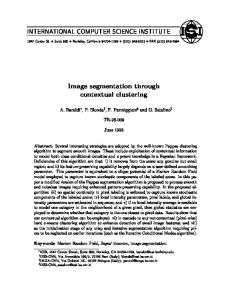
ENDOSCOPIC IMAGE SEGMENTATION In modern oncology the photodynamic diagnostics (PDD) is applied for detecting tumours. This type of diagnostics is based on the phenomenon of different fluorescence of cancer tissues (reddish light) and healthy tissues (greenish light) in blue light of laser. Special fluorescent video endoscope, used in PDD, is a source of colour images of examined tissues (Fig.1).

a)

b)

c) Figure 1. Example of endoscopic image segmentation: a) original image I4, b) KM - based segmentation, c) KHM - based segmentation

A representative set of eight colour endoscopic images (I1, …, I8) has been chosen for the experiment. These images had the same spatial resolution (768×576 pixels) and 24-bit colour depth. During tests were used following parameters of clustering techniques: the RGB colour space, the number of clusters k=5 (some arbitrary choice for these images), the number of iterations equal to 15, p=2.5 (KHM) and SD as the initialization method. After image segmentation by clustering (KM, KHM) we evaluated segmentation results with help of described above VM(I) and Q(I) indexes. Table 1 contains the experimental data. Table 1. KM vs. KHM: comparison of segmentation results VM(I) KM KHM Q(I) KM KHM

I1 I2 I3 I4 I5 I6 0.0019 0.0013 0.0025 0.0025 0.0018 0.0020 0.0016 0.0010 0.0022 0.0015 0.0015 0.0018 I1 I2 I3 I4 I5 I6 95755 311723 7822 286546 7203 330159 2869 2426 3339 3556 7417 3612

I7 0.0022 0.0020 I7 4264 4180

I8 0.0022 0.0019 I8 367838 2509

The analysis of data in Tab.1 leads to the conclusion that KHM technique segments better than KM technique. We can observe that VM(I) values are smaller in case of KHM i.e. an image is better clustered by KHM. The second index Q(I), in seven cases out of eight, is considerably smaller for images segmented by KHM technique.

CONCLUSIONS In comparison with classic KM technique, the KHM leads to better results of endoscopic image segmentation. As directions of further research we can propose following ideas: considering pixel neighbourhood information in segmentation process by KHM, comparison KHM results with other techniques e.g. region-based segmentation techniques and with results of manual segmentation by medical doctor.

ACKNOWLEDGMENTS The second author's participation in this work has been partially supported by the Polish Ministry of Science and Higher Education under grant R13 046 02. REFERENCES [1] H.D. Cheng, X.H. Jiang, Y.Sun and J.Wang: Color image segmentation: advances and prospects, Pattern Recognition, 34(2001), 2259-2281. [2] H. Palus: Color image segmentation: selected techniques, In: Lukac R. and Plataniotis K.N., /Eds./: Color image processing: methods and applications, 103-128, CRC Press, Boca Raton, 2006. [3] J. Mac Queen: Some methods for classification and analysis of multivariate observations, Proceedings of the 5th Berkeley Symposium on Mathematics, Statistics, and Probabilities, Berkeley 1967, vol. I, pp. 281-297. [4] B. Zhang, M. Hsu and U. Dayal: K-harmonic means – data clustering algorithm, Technical Report HPL-1999-124, Hewlett Packard Labs, Palo Alto 1999. [5] B. Zhang: Generalized k-harmonic means – boosting in unsupervised learning, Technical Report HPL-2000-137, Hewlett-Packard Labs, Palo Alto 2000. [6] G.J. Hamerly: Learning structure and concepts in data through data clustering, Ph.D. Thesis, University of California, San Diego 2003. [7] M. Borsotti, P. Campadelli, and R. Schettini: Quantitative evaluation of color image segmentation results, Pattern Recognitions Letters 19 (1998), 741-747.