REDUCED−DIMENSION CLUSTERING FOR VEGETATION SEGMENTATION B. L. Steward, L. F. Tian, D. Nettleton, L. Tang
ABSTRACT. Segmentation of vegetation is a critical step in using machine vision for field automation tasks. A new method called reduced−dimension clustering (RDC) was developed based on theoretical considerations about the color distribution of field images. RDC performed unsupervised classification of pixels in field images into vegetation and background classes. Bayes classifiers were then trained and used for vegetation segmentation. The performance of the classifiers trained using the RDC method was compared with that of other segmentation methods. The RDC method produced segmentation performance that was consistently high, with average segmentation success rates of 89.6% and 91.9% across both cloudy and sunny lighting conditions, respectively. Statistical analyses of segmentation performance coupled with three−dimensional visualization of classifier decision surfaces produced insight into why classifier performance varied across the methods. These results should lead to improvements in segmentation methods for field images acquired under variable lighting conditions. Keywords. Cluster analysis, Machine vision, Segmentation, Vegetation detection.
A
n important need for automation of field−level bioproduction processes is the ability to sense biological objects that are key to the functional objective of the process. While many sensing technologies exist, machine vision has been shown to have great potential as a sensor for a variety of field automation tasks such as vehicle guidance (Han et al., 2002), implement guidance (Slaughter et al., 1999), fruit harvesting (Pla et al., 1993), weed control (Tian et al., 1997), and crop stress sensing (Kim et al., 2000). A key step in implementing machine vision systems for vehicle−based sensing applications is robust segmentation of vegetation from background in field images. Monochrome images have been used for such applications. Segmentation of monochrome field scene images is typically accomplished by thresholding the intensity histograms, which typically have bimodal distributions of pixel gray levels. Reid and Searcy (1988) used a Bayes classifier to find the optimal threshold for segmenting near−infrared (NIR) images of crop rows for obtaining guidance information. Benson et al. (2003) adaptively segmented monochrome images of corn rows for harvester guidance. Brivot and Marchant (1996) used two thresholds and spatial processing to segment NIR field images
Article was submitted for review in February 2003; approved for publication by the Information & Electrical Technologies Division of ASAE in December 2003. The authors are Brian L. Steward, ASAE Member Engineer, Assistant Professor, Department of Agricultural and Biosystems Engineering, Iowa State University, Ames, Iowa; Lei F. Tian, ASAE Member Engineer, Associate Professor, Department of Agricultural Engineering, University of Illinois, Urbana, Illinois; Dan Nettleton, Associate Professor, Department of Statistics, Iowa State University, Ames, Iowa; and Lie Tang, Assistant Professor, Department of Agrotechnology and Food Sciences, Wageningen University, Wageningen, The Netherlands. Corresponding author: Brian Steward, Agricultural and Biosystems Engineering Department, Iowa State University, 206 Davidson Hall, Ames, IA 50011; phone: 515−294−1452; fax: 515−294−2255; e−mail:
[email protected].
of transplanted cauliflower plants into background, crop, and weed classes. Color imaging, as contrasted with monochrome imaging, provides a three−dimensional red, green, blue (RGB) data vector for each pixel and has been shown to be an effective means of measuring and characterizing the growth of crop plants (Tarbell and Reid, 1991), estimating leaf cover of crop and weed canopies (Ngouajio et al., 1999), and discriminating between crop and weed plants for weed control (Lamm et al., 2002). For color images, a common segmentation approach is to transform the three−dimensional data associated with each pixel into a one−dimensional index and then to apply histogram thresholding techniques similar to those used for monochrome images. Shiraishi and Sumiya (1996) transformed the RGB components into the NTSC Q chrominance signal. A threshold on this signal was used to classify pixels as either plant or background. Woebbecke et al. (1992, 1995) investigated several different color indices that mapped the three−dimensional color image data to one dimension. Thresholding was then used to segment the images. Meyer et al. (1998) further described a segmentation procedure that used an excess green color index where the threshold was chosen by observing where the “valley” of the excess green histogram occurred in several images. Andreasen et al. (1997) segmented images by thresholding the median filtered histogram of the g−chromaticity coordinate. Another approach to vegetation segmentation in color images has been to incorporate spatial information into the segmentation process. One approach has been to use active contours constrained by an image energy model (Manh et al., 2001). This approach was used to fit contours to the edges of green foxtail seedlings. Benelloch and Rodas (1999) developed a dynamic binary model operating on a normalized difference index (NDI) image for segmentation of crop and weed from a field image. Perez et al. (2000) used two thresholds applied to an NDI histogram to segment field images and morphological dilation for iterative refinement of the segmentation.
Transactions of the ASAE Vol. 47(2): 609−616
E 2004 American Society of Agricultural Engineers ISSN 0001−2351
609
In order for a segmentation algorithm to be practical for outdoor vehicle−based sensing, it must automatically divide feature space into vegetation or background classes for particular conditions and provide classification results with a low computational burden. In particular, daylight is an extremely variable light source and can be a confounding factor to a machine vision system that is designed to operate in outdoor conditions. Daylight varies in illuminance and illuminant color. Typical daylight illuminance varies from 102,000 lux (lumens/m2) under direct sunlight to 1000 lux under cloudy conditions (Williamson and Cummins, 1983), which is greater than the dynamic range of a CCD camera. Thus the aperture or exposure must be adjusted to compensate for the effects of intensity variation. Illuminant color of daylight is often represented by its correlated color temperature (CCT). The CCT of daylight varies depending on the sun altitude angle and as a function of cloud cover (Wyszecki and Stiles, 1982). Pla et al. (1993) developed a color segmentation algorithm for locating citrus fruits for robotic harvesting under outdoor lighting conditions. This segmentation algorithm was based on the dichromatic reflection model (Klinker, 1993). The polar coordinates for each pixel’s color vector were calculated. Then, working in polar coordinate directional space, the polar angle relative to a white illuminant was calculated. Class thresholds based on the polar angle in the directional space were used to segment pixels into various classes. Tian and Slaughter (1998) developed a color image segmentation algorithm that addressed both issues of lighting variation and real−time performance. First, each pixel vector was transformed to the chromaticity coordinates associated with it. To minimize user intervention and to make the training process as automatic as possible, k−means cluster analysis (MacQueen, 1967) was applied to a sample of pixel chromaticity coordinates from the training image. Then the user determined which clusters should be associated with plant or background classes. Second−order class statistics were then estimated and used to determine the Bayes discriminant functions for each class, resulting in a Bayes classifier that divided RGB color space into plant and background color regions. Using the classifier, a look−up table (LUT) that mapped each color combination to background or plant classes was generated. The LUT was used for real−time segmentation of field images. For cluster analysis to effectively group pixels with similar colors, the effect of large intensity variance must be minimized. Tian and Slaughter (1998) thus mapped pixel values to chromaticity coordinates and performed cluster analysis in the plane represented by them. Further investigations (Steward and Tian, 1998) found that this method resulted in incorrect segmentation of low−intensity pixels due to transformation instability for these colors (Kender, 1976). A linear transformation that separated color information from intensity was investigated. Use of this transformation suggested that more clusters should be used, even though the data should be divided into two clusters corresponding to vegetation and background classes (Steward and Tian, 1998). In addition, the use of four or more clusters required user input to associate clusters with the background and vegetation classes based on visual observation. It is desirable for this procedure to be unsupervised to eliminate the need for human input. These limitations provided motivation for the development of the reduced−dimension clustering technique.
610
The goal of this research was to further understand vegetation segmentation algorithms for color field images. Specific objectives were to: (1) develop an improved method, the reduced−dimension clustering (RDC) algorithm, for training a Bayes classifier for vegetation segmentation, (2) compare the performance of several Bayes classifiers with those generated with the RDC, and (3) develop visualizations of classifier decision surfaces in RGB color space to better understand classifier strengths and weaknesses.
MATERIALS AND METHODS DATA COLLECTION AND HAND SEGMENTATION A 3−CCD camera (model XC−003, Sony America, New York, N.Y.) was used to acquire images of two rows of soybeans and the interrow area. The camera was mounted at a height of 3.35 m (11 ft) on a custom−made camera boom (fig. 1) for a Patriot XL sprayer (Tyler Industries, Benson, Minn.). A 12.5 to 75 mm, F 1.2 zoom lens (model M6Z 1212, Computar, CBC (America) Corp., New York, N.Y.) was used to image a 1.1 × 0.8 m (43 × 33 in.) area with a 12.5 mm zoom setting. Images were taken with the aperture set at F 8 for sunny conditions and F 5.6 for overcast sky conditions with the shutter speed at 1/250 s. The color temperature was set at 5600 K with manual white balance set at a −2 dB blue channel gain and a −20 dB red channel gain. The camera had a resolution of 768 × 494 pixels. The Y/C (S−video) output of the camera was routed to a PXC200 (Imagenation, Beaverton, Ore.) color frame grabber installed in a Pentium−based portable computer. The frame grabber had a resolution of 640 × 486 pixels and converted the analog video signal to 24−bit digital color images. Each pixel corresponded to an area approximately 0.002 × 0.002 m. The images were grabbed when the computer was triggered by the user and written to Windows bitmap files with 24−bit color resolution. Images were taken while the sprayer was moving with a slow forward travel speed of 0.6 km/hour (0.4 miles/ hour) to minimize motion effects. Two sets of images were acquired on June 29, 1998: one set consisting of 129 images in the morning under overcast sky conditions, and the other set consisted of 138 images in the afternoon under sunny conditions. Four images were selected from the cloudy condition image set, and another four were selected from the sunny condition image set for further analysis. These eight images were manually segmented by a person painting the vegetation pixels in the images with a common color using Paint Shop Pro (Jasc Software, Inc., Minneapolis, Minn.). The great time and tedium required to do this process limited the number of images in the data set.
Figure 1. Physical location of the Sony XC−003 camera used to collect the images analyzed in this research.
TRANSACTIONS OF THE ASAE
Figure 2. Scatter plot of pixel values in RGB color space for a field image acquired in (a) cloudy and (b) sunny lighting conditions. The lower cylindrical cluster in each plot consists mainly of vegetation pixels.
REDUCED−DIMENSION CLUSTERING The data from the field images tended to cluster into two cylindrical regions emanating from the origin of RGB color space (fig. 2). The background pixel cylinder axis was collinear with the intensity axis. The plant pixel cylinder had an axis whose angle with the green coordinate vector was smaller than that of the background pixel cylinder. Chromaticity coordinates map to color vectors starting at the origin of RGB color space (Steward, 1999). These vectors can be described by a spherical coordinate system (Pla et al., 1993). In a real case, sensor noise and variations in object color will cause the points to deviate from a straight line, leading to a cylindrical cluster. These observations were consistent with the dichromatic reflection model (Klinker, 1993; Shafer, 1985). Since objects of different colors group along color vectors, it would be expected that a segmentation algorithm that grouped data according to this structure would have better performance. Reduced−dimension clustering (RDC) is a K−means− based algorithm that clusters data to color vectors using perpendicular distance to a vector as the proximity index, instead of clustering to points in color space. Each color vector has its endpoint fixed at the origin and is free to rotate about the origin as clustering takes place (fig. 3). The procedure is called “reduced−dimension clustering” because the proximity index ignores the variation of the data along the length of the cluster vector. Intensity variation thus has little influence on clustering. However, the intensity of each data point is first compared with a minimum intensity threshold. If the intensity is lower than the threshold, then the data point is placed in a low−intensity cluster since low−intensity pixels have little color information. The RDC algorithm calculates distances between individual data points and each cluster line by the following equation: z ik = x i − (x i • u k )u k
(1)
where zik = perpendicular distance between data point i and cluster line k xi = vector from the origin to the ith data point uk = unit vector associated with cluster line k. Each data point was grouped with the nearest cluster line based on this calculation. After each iteration, each cluster line angle was updated with the average of the angles of all data points vectors associated with that cluster line, weighted by the
Vol. 47(2): 609−616
Figure 3. The perpendicular distance from each cluster line to each data point is calculated. Each data point is clustered with the closest cluster line.
magnitude of those vectors. This weighting was used since the color signal−to−noise ratio was greater for the higher−intensity pixels. Each angle was then used to find the three components of the vector. The components of the kth cluster line vector were thus calculated by:
y jk
1 = cos N ∑k x i i =1
Nk ∑ xi θij i =1
(2)
where yjk = jth component of the kth cluster line vector Nk = number of data points clustered in the kth cluster qij = angle between xi and the jth axis where j ∈ {R, G, B} . qij is calculated by the equation:
611
xij θij = cos −1 x i
(3)
where xij is the projection of xi on the jth axis. Clustering continued until the algorithm converged to a particular set of cluster line orientations with no change in orientation from the previous orientation (fig. 4). SEGMENTATION PERFORMANCE COMPARISON Bayes classifiers were trained using four different methods on the eight images, resulting in 4 × 8 = 32 different classifiers. The first method transformed the pixel data into chromaticity coordinates. This transformation is a normalization by pixel intensity, and thus the method was called NOR (Tian and Slaughter, 1998). K−means cluster analysis was performed in the chromaticity coordinate plane with four cluster centers. One cluster center was associated with the vegetation class in every training image except two cloudy images with high vegetation densities where two clusters better represented the vegetation class than one. After pixel labeling, each classifier was trained in the chromaticity coordinate plane. Two other methods were similar to the first method, but a linear coordinate transformation was used to map the data into a coordinate system that concentrated the variation in color into two coordinates that spanned the color plane (Steward, 1999). The transformation to one coordinate was equivalent to the excess green color index (Woebbecke, 1995). K−means cluster analysis was performed with four cluster centers, and classifier training was done in the resulting color plane. One method associated one cluster with the plant class and was
Figure 4. Flowchart of the reduced−dimension clustering algorithm. At completion, each data point is assigned to a cluster.
612
called EG1 for excess green−one cluster. For the other, called EG2, two clusters were associated with the plant class. The last method, called RDC, used the RDC algorithm with three clusters. A vector for the plant class represented one cluster, and another represented the background class. The third cluster was composed of data points with intensities less than a threshold of 15. In contrast to the other methods, the RDC algorithm did not require user intervention since there was a smaller angle between the cluster vector representing the plant class and the green coordinate axis, making association with the plant class easily automated. The eight images were segmented by each of the 32 classifiers. Each segmented test image was compared pixel−by−pixel with the corresponding hand−segmented image. From these comparisons, the segmentation success rate (SSR) of each test image was computed. The SSR was defined by: SSR =
PT + BT − (I P + I B ) PT + BT
(4)
where PT = number of pixels manually segmented as plant in the image BT = number of pixels manually segmented as background in the image IB = number of pixels incorrectly segmented as back ground based on the hand−segmented image IP = number of pixels incorrectly segmented as plant based on the hand−segmented image. Thus, for any image and classifier, SSR was the ratio of the number of pixels classified in agreement with hand segmentation relative to the total number of pixels. STATISTICAL ANALYSIS Mixed linear model analyses of the SSR data were performed using the SAS Mixed Procedure (Ver. 8.2, SAS Institute, Inc., Cary, N.C.). A standard approach to analysis described in Kuehl (2000, pp. 232−255) was used. For each combination of segmentation method, training image, and test image, the SSR score was computed, resulting in a total of 4 × 8 × 8 = 256 data points. Scores for identical training and test images were excluded to avoid an exaggeration of segmentation performance leaving a total of 224 data points for mixed linear model analysis. Segmentation method (NOR, EG1, EG2, RDC), lighting condition of the training image (cloudy vs. sunny), and lighting condition of the test image (cloudy vs. sunny) were included as fixed main effects. The four cloudy and four sunny images used in the study were viewed as samples from broader image populations to which our results were to be generalized. Thus, training image nested within training condition and test image nested within test condition were modeled as random factors. All interactions were included in the mixed model. Interactions involving one or more random terms were modeled as random effects. The method−of−moments approach was used to compute all standard errors and determine appropriate error terms for all tests of interest. Satterthwaite’s method (Satterthwaite, 1946) was used to approximate degrees of freedom for error terms formed by a linear combination of mean squares. In order to achieve roughly constant error variance required by the statistical methods, the SSR scores were transformed by the arcsine−square−root transformation (Kuehl, 2000, p. 134) prior to mixed linear model analysis. Identical analyses were
TRANSACTIONS OF THE ASAE
conducted on the untransformed data, which led to the same conclusions. Results were reported on the original SSR scale for ease of interpretation. VISUALIZATION Matlab (Mathworks, Natick, Mass.) script language was used to generate graphical representations of the decision surfaces associated with the classifiers. RGB color space was sampled at five intensity level intervals, and at each sample, the value of each discriminant function was calculated. The largest discriminant function value associated with a plant class was subtracted from the values of the background class discriminant functions. A scalar field was thus generated. Color space regions more likely to be background pixels had negative values, and those more likely to be plant pixels had positive values. Isosurfaces at the boundaries of these regions represented classifier decision surfaces.
RESULTS AND DISCUSSION Significant interaction between segmentation method and test condition was detected (F3,24.4 = 12.26, p < 0.0001). Thus segmentation methods were compared separately for cloudy and sunny test conditions. Significant differences among the four methods were detected under cloudy test conditions (F3,28.8 = 6.47, p < 0.005) and under sunny conditions (F3,28.8 = 8.04, p < 0.001). Under cloudy test conditions, EG2 exhibited the best performance followed by RDC, NOR, and EG1. When controlling the overall probability of one or more type I errors using a Bonferroni adjustment to account for six pairwise comparisons among means, both EG2 and RDC had significantly better performance than EG1 at the 5% significance level. All other differences were not significant at the 5% level (table 1). Under sunny test conditions, RDC exhibited the best performance followed by EG1, NOR, and EG2. The RDC, EG1, and NOR means were not significantly different from one another, but each of these methods had a mean that was significantly greater than the EG2 mean (table 2). Again, the Bonferroni method was used to bound the probability of one or more type I errors at 5%. The variation in performance of the EG1 and EG2 methods across lighting conditions was a salient result. For these two Table 1. Segmentation performance under cloudy conditions. Method Average SSR (%)[a] EG2 RDC NOR EG1 [a]
90.9 a 89.6 a 85.2 ab 81.9 b
Letters indicate methods that are not significantly different from one another when the probability of one or more type I errors is controlled at the 5% level. Table 2. Segmentation performance under sunny conditions. Method Average SSR (%)[a] RDC EG1 NOR EG2
[a]
91.9 a 90.5 a 90.1 a 81.8 b
Letters indicate methods that are not significantly different from one another when the probability of one or more type I errors is controlled at the 5% level.
Vol. 47(2): 609−616
methods, a linear transformation mapped the data to two coordinates that spanned the color plane orthogonal to the intensity vector. While this linear transformation minimized the effect of intensity variation without introducing the non−ideal effects associated with chromaticity transformation, it also resulted in Bayes decision surfaces that were parallel to the intensity axis. Since vegetation pixels were clustered along a vector that was not parallel to the decision surfaces, one cluster often contained a mixture of vegetation and background pixels. Thus this procedure typically resulted in one cluster corresponding to the vegetation class, two corresponding to the background, and the remaining cluster with an uncertain classification. In the EG1 method, only one cluster consisting of the most saturated green pixels was associated with the vegetation class. This association resulted in the decision surface between vegetation and background pixels being further from the intensity axis than that produced by the EG2 method. Under cloudy conditions, EG1 had lower performance because the vegetation pixels tended to have a lower intensity and were thus closer to the intensity vector in the vegetation cluster (fig. 2a). More vegetation pixels were on the background side of the decision surface and were thus segmented incorrectly. However, under sunny conditions, the intensity of the vegetation pixels tended to increase and be further away from the intensity axis (fig. 2b). Since the decision surface was parallel to the intensity axis, more of the plant pixels were on the plant side of the decision surface, resulting in higher segmentation performance. The opposite effect occurred with the EG2 method in which two clusters were associated with the plant class, resulting in a decision surface that was again parallel, but closer, to the intensity axis. The three−dimensional isosurface plots produced for classifier visualization (fig. 5) provided visual evidence for the above explanation. For both the EG1 (fig. 5b) and EG2 (fig. 5c) methods, the decision surfaces were parallel to the intensity axis. The only difference between the two decision surfaces was the additional region associated with the background class in the EG1 decision surface as compared with the EG2 decision surface. The decision surfaces associated with the NOR method (fig. 5a) were not parallel to the intensity axis but met at a point at the origin. This decision surface collapsed to a point, resulting in unstable classification for low−intensity pixels as observed earlier (Steward and Tian, 1998). The RDC decision surface was also not parallel to the intensity axis and produced a decision surface that wrapped around the vegetation cluster. The use of a low−intensity cluster near the origin effectively classified low−intensity pixels as pixels with indistinguishable color. For the classifiers developed in this research, this cluster was associated with the background class under the assumption that the background would tend to consist of darker pixels. The pixels in this cluster could, however, be classified as either plant or background based on their connectivity to other background or plant pixels. For all of the decision surfaces, decision surfaces existed behind the background class in the three−dimensional plots, indicating that pixels in these regions would also be classified as vegetation. These decision surfaces are produced by the other half of the typical hyperbolic surface produced by the Bayes classifier. These surfaces do not typically cause segmentation errors because they only classify highly satu−
613
(a)
(b)
(c)
(d)
Figure 5. Examples of decision surfaces produced by each classifier: (a) NOR classifier, (b) EG1 classifier, (c) EG2 classifier, and (d) RDC classifier. Pixels in the solid region of the color space are segmented as background. Those in the hollowed out region are segmented as vegetation.
rated reds or purples (i.e., colors that do not typically appear in natural agronomic field scenes) as plants. The performance results were also confirmed by observing binary images resulting from segmentation with each of the methods for cloudy conditions (fig. 6) and sunny conditions (fig. 7). In these images, visual assessments supported the above observations. For example, the binary images produced with EG1 segmentation revealed the loss of plant pixels for both cloudy and sunny cases (figs. 6c and 7c) when compared
with the images produced by EG2 (figs. 6d and 7d). The EG2 method had poor segmentation performance under sunny conditions because many background pixels were misclassified as vegetation. In the case of the NOR method, the low−intensity pixels associated with cracks in the soil tended to be classified as plants and were visible as contorted lines in both binary images (figs. 6b and 7b). The segmentation results of the RDC method provided good segmentation results consistently across both conditions (figs. 6e and 7e).
(a)
(b)
(d)
(e)
(c)
Figure 6. Segmentation of an example image acquired under cloudy conditions by the following methods: (a) hand segmentation, (b) NOR, (c) EG1, (d) EG2, and (e) RDC.
614
TRANSACTIONS OF THE ASAE
(a)
(b)
(d)
(e)
(c)
Figure 7. Segmentation of an example image acquired under sunny conditions by the following methods: (a) hand segmentation, (b) NOR, (c) EG1, (d) EG2, and (e) RDC.
CONCLUSIONS Through this work, the following conclusions can be drawn: S The reduced−dimension clustering method was developed based on theoretical considerations about the shape of data clusters in RGB color space from field images and resulted in Bayes classifiers that produced high segmentation performance consistently with average SSR values of 89.6% and 91.9% across both cloudy and sunny lighting conditions, respectively. S Statistical analysis of classifier performance produced results that were consistent with qualitative assessments of binary images produced by the classifiers. S Visualization of classifier decision surfaces increased understanding of how the color space was being divided and provided insight into the meaning of the segmentation performance from the different segmentation methods. ACKNOWLEDGEMENTS This research of the Iowa Agriculture and Home Economics Experiment Station, Ames, Iowa, Project No. 3612, was supported by Hatch Act and State of Iowa funds and the Illinois Council for Food and Agricultural Research under Award No. C−Far 1−5−9528 and the USDA National Need Graduate Student Fellowship Program. Any opinions, findings, and conclusions or recommendations expressed in this publication are those of the authors and do not necessarily reflect the views of the sponsors.
REFERENCES Andreasen, C., M. Rudemo, and S. Sevestre. 1997. Assessment of weed density at an early stage by use of image processing. Weed Research 37(1): 5−18. Benlloch, J. V., and A. Rodas. 1999. Dynamic model to detect weeds in cereals under actual fields conditions. In Proc. SPIE 3543: Precision Agriculture and Biological Quality, 302−310. G. E. Meyer and J. A. DeShazer, eds. Bellingham, Wash.: SPIE.
Vol. 47(2): 609−616
Benson, E. R., J. F. Reid, Q. Zhang. 2003. Machine vision−based guidance system for an agricultural small−grain harvester. Trans. ASAE 46(4): 1255−1264. Brivot, R., and J. A. Marchant. 1996. Segmentation of plants and weeds for a precision crop protection robot using infrared images. IEEE Proc. on Vision, Image, and Signal Processing 143(2): 118−124. Han, S., M. A. Dickson, B. Ni, J. F. Reid, and Q. Zhang. 2002. A robust procedure to obtain a guidance directrix for vision−based vehicle guidance systems. In Proc. Automation Technology for Off−Road Equipment Conference, 317−326. Q. Zhang, ed. St. Joseph, Mich.: ASAE. Kender, J. 1976. Saturation, hue, and normalized color: Calculation, digitization effects, and use. Tech. Report. Pittsburgh, Pa.: Carnegie−Mellon University, Department of Computer Science. Kim, Y., J. F. Reid, A. Hansen, and M. Dickson. 2000. Evaluation of a multi−spectral imaging system to detect nitrogen stress of corn crops. ASAE Paper No. 003128. St. Joseph, Mich.: ASAE. Klinker, G. J. 1993. A Physical Approach to Color Image Understanding. Wellesley, Mass.: A. K. Peters, Ltd. Kuehl, R. O. 2000. Design of Experiments: Statistical Principles of Research Design and Analysis.2nd ed. Pacific Grove, Cal.: Duxbury Press. Lamm, R. D., D.C. Slaughter, and D. K. Giles. 2002. Precision weed control system for cotton. Trans. ASAE 45(1): 231−238. MacQueen, J. 1967. Some methods for classification and analysis of multivariate observations. In Proc. 5th Berkeley Symp. on Mathematical Statistics and Probability, Vol 1: 281−297. Berkeley, Cal.: University of California Press. Manh, A. G., G. Rabatel, and M. J. Aldon. 2001. Weed leaf image segmentation by deformable templates. J. Agric. Eng. Research 80(2): 139−146. Meyer, G. E., T. Mehta, M. F. Kocher, D. A. Mortensen, and A. Samal. 1998. Textural imaging and discriminant analysis for distinguishing weeds for spot spraying. Trans. ASAE 41(4): 1189−1197. Ngouajio, M., G. D. Leroux, and C. Lemieux. 1999. Influence of images recording height and crop growth stage on leaf cover estimates and their performance in yield prediction models. Crop Protection 18(8): 501−508.
615
Perez, A. J., F. Lopez, J. V. Benlloch, and S. Christensen. 2000. Colour and shape analysis techniques for weed detection in cereal fields. Computers and Electronics in Agric. 25(3): 197−212. Pla, F., F. Juste, F. Ferri, and M. Vicens. 1993. Colour segmentation based on a light reflection model to locate citrus fruits for robotic harvesting. Computers and Electronics in Agric. 9(1): 53−70. Reid, J. W., and S. W. Searcy. 1988. An algorithm for separating guidance information from row crop images. Trans. ASAE 31(6): 1624−1632. Satterthwaite, F. E. 1946. An approximate distribution of estimates of variance components. Biometrics 2: 110−114. Shafer, S. A. 1985. Using color to separate reflection components. Color Research and Applic. 10(4): 210−218. Shiraishi, M., and H. Sumiya. 1996. Plant identification from leaves using quasi−sensor fusion. J. Manufacturing Science and Eng., Trans. ASME 118(3): 382−387. Slaughter, D. C., P. Chen, and R. G. Curley. 1999. Vision guided precision cultivation. Precision Agric. 1(2): 199−216. Steward, B. L. 1999. Sensing and control for real−time machine vision−based selective herbicide application under outdoor field condition. Unpublished PhD diss. Urbana, Ill.: University of Illinois at Urbana−Champaign.
616
Steward, B. L., and L. F. Tian. 1998. Real−time weed detection in outdoor field conditions. In Proc. SPIE 3543: Precision Agric. and Biological Quality, 266−278. G. E. Meyer and J. A DeShazer, eds. Bellingham, Wash.: SPIE. Tarbell, K. A., and J. R. Reid. 1991. A computer vision system for characterizing corn growth and development. Trans. ASAE 34(5): 2245−2255. Tian, L. F., and D. C. Slaughter. 1998. Environmentally adaptive segmentation algorithm for outdoor image segmentation. Computers and Electronics in Agric. 21(3): 153−168. Tian, L. F., D. C. Slaughter, and R. F. Norris. 1997. Outdoor field machine vision identification of tomato seedlings for automated weed control. Trans. ASAE 40(6): 1761−1768. Williamson, S. J., and H. Z. Cummins. 1983. Light and Color in Nature and Art. New York, N.Y.: John Wiley and Sons. Woebbecke, D. M., G. E. Meyer, K. Von Bargen, and D. A. Mortensen. 1992. Plant species identification, size, and enumeration using machine vision techniques on near−binary images. In Proc. SPIE 1836: Optics in Agriculture and Forestry, 208−212.J. A DeShazer and G. E. Meyer, eds. Bellingham, Wash.: SPIE. Woebbecke, D. M., G. E. Meyer, K. Von Bargen, and D. A. Mortensen. 1995. Color indices for weed identification under various soil, residue, and lighting conditions. Trans. ASAE 38(1): 259−269.
TRANSACTIONS OF THE ASAE