The control system considers two loops in cascade, an internal loop solving the robot' ... by roll (θ) and pitch (Ï) angles respectively, and linear displacement along the z axis. (elevation) ... So, the moving platform can simulate different sceneries ..... each task space coordinate, with the form for the height,. [ h(k + 1) h(k + 2). ].
5 Kinematic Task Space Control Scheme for 3DOF Pneumatic Parallel Robot Luis Hernández1 , Eduardo Izaguirre2 , Ernesto Rubio3 , Orlando Urquijo4 and Jorge Guerra5 1,2,3,4 Automation,
Robotic and Perception Group (GARP). Universidad Central de Las Villas (UCLV) 5 SIMPRO Cuba
1. Introduction Parallel robots have received special attention of the systems and control community based on its high force-to-weight ratio and widespread applications (Merlet, 2006). The control schemes for a parallel robot can be divided into two strategies: joint space control (Wang et al., 2009), (Gupta et al., 2008) and task-space control (Ting & Chen, 1999). The joint space control scheme is based on the information of each actuator length and can be implemented as a decoupled independent single-input single-output (SISO) control systems for each actuator, with in general, poor compensation of the uncertainties. On the other hand, a task space controller has a potential to provide a better control for the parallel robot under system uncertainties: inertia, modeling error, friction, etc. Nevertheless this type of control scheme needs the direct measurement of system task space state (Gao et al., 2008) or task space state estimation, normally cumbersome. Task space control schemes have been presented for direct inverse dynamics control, with joint space dynamic model compensation (Feng, 1995) or task space dynamics model compensation,(Li & Xu, 2008), including vision based computed torque in task space control (Paccot et al., 2008). Many of this schemes have been proved by simulation or in laboratory testbed, but not commonly on industrial motion platform. The goal of this work is to improve the performance of the control system of an industrial 3DOF pneumatic parallel platform, used by SIMPRO company who develop driver simulator. The solution of the control problem in the joint space of the parallel structure with pneumatic actuators have been obtained by Rubio (Rubio et al., 2009), using a decoupled control based on actuator lineal model around the operational point. But the performance of this scheme is strongly dependent of the precision of the kinematic model and dynamic uncertainties. The solution proposed, the kinematic task space control, is based on the direct measurement of system task space state. The control system considers two loops in cascade, an internal loop solving the robot’ joint control (q), and an external loop implementing the task space control (x). The proposed control philosophy, based on robot kinematic model, have been used by Hernández (Hernández et al., 2008a),(Hernández et al., 2008b) in vision-based 2D and 3D control of robot manipulators. In this scheme type, for digital implementation, it is possible
68
Object Tracking
to approximate the dynamic effect of the internal loop as an external loop time delay (Corke, 1996), (Hernández et al., 2010) and (Bonfe et al., 2002). In this conditions a stability analysis in discrete time is developed. To illustrate the proposed controller, the control system stability and its performance, both co-simulation results via MATLAB/Simulink and ADAMS, as well as experimental results using the SIMPRO 3DOF pneumatic parallel robot are presented. Experimental results confirm the expected step response in the task space, with good time performance and zero steady-state error. The control scheme presented open a new research field in the task space control with algorithms for the solution of, trajectory control, feed-forward control, etc.
2. Parallel robot model As shown in Fig. 1, the robotic system considered consist of a 3DOF parallel manipulator controlled by pneumatic actuators. The parallel robot is produced by SIMPRO for driving simulator purpose, the robot have sensors to measurement the joint displacements and task space states. The basic mathematical description of this system consists of the parallel robot kinematics and dynamic model and also the actuator models.
Fig. 1. SIMPRO 3DOF pneumatic driver simulator parallel platform 2.1 Robot kinematics model
The same manner that serial manipulators, kinematics relations of parallel robots gives the relationship between the joints variables q and the corresponding position ( x, y, z) and angular orientation (θ, ϕ, ψ) of center of mass of mobile platform in cartesian space. For an n-axis parallel structure, the forward kinematic (FK) solution T could be numerically computed according with the number of joints of kinematic architecture (Merlet, 2006). Generic mathematical representation of forward kinematics could be: x=
�
xyzθϕψ
�T
= f ( q1 , q2 , . . . , q n ) = T
(1)
For parallel robots the complexity of FK equations increase noteworthy with the numbers of degree of freedom, the solution is non-unique and numerical methods are currently used to obtained the solutions, unfortunately there is no known algorithm that allows the
Kinematic Task Space Control Scheme for 3DOF Pneumatic Parallel Robot
69
determination of the current pose of the platform among the set of solutions. Furthermore, the computation times involved in FK algorithms are still too large for use in a real time application (Merlet, 2006). For robot path planning, the inverse kinematic (IK) expressions T−1 gives the joint coordinates q required to reach the specified pose of mobile platform. The mathematical expression of inverse kinematics can be written as: q=
�
q1 q2 . . . q n
�T
= g( x, y, z, θ, ϕ, ψ) = T−1
(2)
Schematic of the 3-DOF parallel robot under study is shown in Fig. 2. The system consists of a fixed base connected to moving platform by three actuated kinematics chains, following the RPSU-2SPS architecture. A base coordinate frame designated as Oxyz frame is fixed at the center of the base with its z-axis pointing vertically upward and the x-axis pointing backwards of the platform. Similarly a moving coordinate frame Px � y� z� is assigned to the center mass of the moving platform, with the z� -axis normal to the mobile platform. By simplicity the directions of both z and z� axes are pointing in the same unit vector.
Fig. 2. The RPSU-2SPS kinematics structure of the 3-DOF motion platform. The actuators are double effect electro-pneumatic cylinders whose lineal displacements produce the 3-DOF of robot, consisting in two rotations around the x � and y� axes, represented by roll (θ) and pitch (ϕ) angles respectively, and linear displacement along the z� axis (elevation), defined by the variable h. So, the moving platform can simulate different sceneries in correspondence with virtual reality world that is shown in LCD display located inside the cabin with is supported by mobile platform. This type of applications are developed by SIMPRO company. The vectorial formulation allows us to simply construct a set of equations which contains the same number of equations as the unknown variables. According with this procedure a closed vector cycle is constituted between the points Ai and Bi in correspondence with the illustration represented in Fig. 3. Establish the inverse kinematics model is essential for the position control of robot. Then, for each kinematics chain, a vectorial function can be formulating by expressing the actuated joint coordinates as a function of cartesian coordinates (x) whose define the pose of the mobile
70
Object Tracking
Fig. 3. Representation of closed loop vectors for each active legs. platform. According to equation (2) is necessary to found the relation Ai Bi = g(x) in order to calculate the inverse kinematics model of robot. Considering the schematic presented in Fig. 3, follows that: p + bi = ai + Li
(3)
p = OP = [ Px , Py , Pz ] T − [Ox , Oy , Oz ] T
(4)
ai = ||OAi ||2
(5)
bi = |PBi ||2
(6)
Li = ||Ai Bi ||2
(7)
where:
The position vector of the mobile platform with reference to the fixed frame is defined by the vector p = OP, that is, platform position in cartesian space is defined by z� coordinates of point P. Consequently the orientation of mobile platform is determined by θ and ϕ angles. Due to mechanical restrictions of robotic structure, the yaw angle is zero (ψ = 0), then, the rotation matrix is defined by only the roll and pitch angles. Following the ZYX convention for Euler angles, the rotation matrix can be computed by the expression: ⎡ ⎤ cos( ϕ) sin( ϕ)s(θ ) sin( ϕ)c(θ ) xyz ⎦ 0 cos(θ ) −sin(θ ) R x� y� z� = R BA = ⎣ (8) −sin( ϕ) cos( ϕ)sin(θ ) cos( ϕ)cos(θ ) It can be easily seen that the described architecture is characterized by 3-DOF’s in cartesian space; in general case the appropriated linear displacements of each actuator are related with changes of orientation and elevation of the mobile platform. Then, the location of the moving platform can be described by a position vector p and a rotation matrix R BA . By construction the fixed reference frame coordinates of Ai ’s points are known, while the coordinates of Bi ’s may be determined from the position and orientation of mobile platform. Hence the vector Ai Bi plays an important role in the solution of inverse and direct kinematics problems.
Kinematic Task Space Control Scheme for 3DOF Pneumatic Parallel Robot
71
Considering equations (3) to (7) and (8), the general closed-loop equation for the SIMPRO motion simulator platform as the form: Ai Bi = OP + R BA PBi − OAi
(9)
The central kinematics chain (corresponding with the actuator No. 1) have different architecture for the others, and then, new additional equation is necessary to be considered: A1 B1 = A1 C1 + C2 C1 − B1 C2
(10)
Substituting (10) in (9) and considering the all closed loop equations for each active leg, we have: A1 C1 = OP + R BA PB1 − OA1 + B1 C2 + C2 C1
(11)
A2 B2 = OP + R BA PB2 − OA2
(12)
A3 B3 = OP + R BA PB3 − OA3
(13)
The design of robot included two additional rigid bodies interconnected between the base and the moving platform to provide mechanical stability and stiffness of robotic structure. This particular characteristic produce a curvilinear movement of mobile platform during elevation as is shown in Fig.4.
Fig. 4. Additional displacement �x of mobile platform during elevation. Consider the straight line between points PP� is defined by equation z = mx + b, where m and b are the slope and intercept respectively, additionally the circle with center in ( xc ; zc ) and ratio r is described by the circumference equation ( x − xc )2 + (z − zc )2 = r2 . Then, the movement along z-axis as a function of displacement of moving platform in the x-axis is calculated from: � 2m(b − zc ) − 2xc 2 4k1 (14) − Δz = m 1 + m2 1 + m2 where: k1 = xc2 + z2x + b(b + 2zc ) − r2 Because equation (14) compute the new coordinates of Bi ’s points of mobile platform during elevation, itt’s incorporate to the solution of IK problem.
72
Object Tracking
Given the initial position Loi of limbs it is possible to calculate the displacements of lineal actuators qi according to (15), considering the scheme of Fig. 5. qi = Li − Loi
(15)
Fig. 5. Illustration of initial position of actuators in each robott’s limbs. 2.2 Robot dynamics model
In the absence of friction or other disturbances, the dynamics of parallel robot can be written as (Merlet, 2006) M x (x)x¨ + C x (x, x˙ )x˙ + G x (x) = J T f = f x
(16)
where: M x (x) x C x (x, x˙ ) G x (x) J f
n × n symmetric positive definite manipulator inertia matrix n × 1 vector of space displacements n × n centripetal and Coriolis matrix n × 1 vector of gravitational term n × n robot Jacobian matrix n × 1 vector of applied joint forces
In other hand the dynamic model in joint space can have, in some configuration, the form, (Li & Xu, 2008) M(q)q¨ + C(q, q˙ )q˙ + g(q) = f
(17)
where: M(q) n × n symmetric positive definite manipulator inertia matrix q n × 1 vector of joint displacements C(q, q˙ ) n × n centripetal and Coriolis matrix G(q) n × 1 vector of gravitational term f n × 1 vector of applied joint forces 2.3 Pneumatic Actuators Model
Our platform actuators are pneumatic cylinders. To obtain the dynamic model of a pneumatic cylinder, normally (Brun et al., 2000), the following consideration are taken: only viscous friction is present, the temperature is constant and equal in both cylinder chambers and the gas is ideal. Additionally, according Rubio (Rubio, 2009), the influence of the underlap
Kinematic Task Space Control Scheme for 3DOF Pneumatic Parallel Robot
73
characteristic of the valve is considered. Under this conditions, the transfer function of the system, position Y (s) versus control action U (s), is obtained with the form, Y (s) b1 s + b0 = U (s) s ( c3 s3 + c2 s2 + c1 s + c0 )
(18)
Once defined the operating point of the valve, the coefficients ci and bi , are variables in dependent of the position y0 . According the experimental work developed in (Rubio, 2009), a good approximation of equation (18) can be, Gyu(s) =
b s ( s2 + a1 s + a0 )
(19)
where b is the system gain, a1 = 2 ζ˜ ω˜ n and a2 = ω˜ n2 ; where ω˜ n and ζ˜ are respectively the open loop undamped natural frequency and damping ratio of the system. These parameter are not constants, they vary in dependency of the position y0 .
3. Control problem The control problem is formulated as the design of a controller which computes a control signal Δ corresponding to the movement of the robot’s in such a way that the desired task space position be reaches following wanted performances index. 3.1 Control problem formulation
� �T For control the desired state, θd ϕd hd , is moving part. The task state error being defined as: ⎡ ⎤ ⎡ θ˜ y˜ = yd − y = ⎣ ϕ˜ ⎦ = ⎣ h˜
the position of center of mass platform ⎤ ⎤ ⎡ θd θ ϕd ⎦ − ⎣ ϕ ⎦ h hd
which could be calculated at every measurement time and used to move the robot in a direction allowing its decrease. Therefore, the control aims at ensuring that lim y˜ = lim
t→∞
t→∞
�
θ˜
ϕ˜
h˜
�T
=0
We make the as assumptions for the control problem that, only the control problem is evaluated with initial error ξ˜(0) is sufficiently small and there exists a robot joint configuration qd for which ξ d = ξ (qd ). This condition ensures that the control problem is solvable. 3.2 Kinematic task space control
For our control problem formulation, the task space vector of the robot can be measured by external sensors. As such, a direct knowledge of the desired joint position qd is not available. Nevertheless, the desired joints position can be obtained as a result of the estimated control signal Δ and the solution of the kinematics problems. The implemented closed-loop block diagram can be described as shown in Fig. 6. The control system has two loops in cascade, the internal loop solving the robots’ joint control, and the external loop implementing a kinematic task space control.
74
Object Tracking
Fig. 6. Control scheme The inner control loop has an open control architecture; in this architecture it is possible to implement any type of controller. One possibility is to use a non-linear controller in the state variables, called Model Based Computed Torque Control (Yang et al., 2008), having the following control equation, for a robot with n-DOF, τ = M(q)[q¨d + Kvi q˙ + K pi q˜ ] + C(q, q˙ )q˙ + G(q)
�n×n
Where K pi ∈ and Kvi ∈ �n×n are the symmetric positive-definite matrices and q˜ = q − qd . It is possible to demonstrated that with this configuration the system behaves in a closed loop as a linear multivariable system, decoupled for each robot’s joint, suggesting that the matrices could be specified as: K pi = diag{ω12 , . . . , ωn2 } Kvi = diag{ω1 , . . . , ωn } In this way each joint behaves as a critically damping second order linear system with bandwidth ωi . The bandwidth ωi determines the speed of response of each joint. In such way the dynamic effect of the internal loop could be independent with regard to the external loop, being under the conditions that: q(t) = qd (t)
∀t > 0
(20)
This control philosophy have been used by Hernández (Hernández et al., 2008b) in vision-based 3D control of robot manipulators. Nevertheless, control systems is implemented fully as a sampled data systems. Åström (Åström K. J.and Wittenmark, 1990) established that the sampling rate of digital control systems should be between 10 and 30 time the desired closed loop bandwidth. For the case low cost driver simulators system the close loop bandwidth should be around 0.1 Hz. A sampling rate for the external loop between 100 to 30ms is excellent for the wanted close loop bandwidth of the system. In the analysis of the control problem in the field of digital control systems, other dynamic representation can be made for the internal loop, of the robot control system could be as one or two delay units of the external loop (Corke, 1996) or for the robot (Bonfe et al., 2002). Using this consideration we modify Equation (20) as, q ( k ) = q d ( k − 1)
∀k > 0
(21)
Kinematic Task Space Control Scheme for 3DOF Pneumatic Parallel Robot
75
4. Stability analysis A simple I controller can be used in this control scheme (Hernández et al., 2008b), for that case the control law can be given by: Δ = KI
Where K I ∈ �2×2 is the symmetric integral matrix: ⎡ K I1 0 K I2 KI = ⎣ 0 0 0
ξ˜
(22) ⎤ 0 0 ⎦ K I3
(23)
Similarity as the visual control work (Hernández et al., 2010), Δ can be interpreted as the coordinates increment in the task space as a result of the direct mensuration of center of mass of moving platform position. Solving the inverse kinematics problem T −1 it is possible to obtain qd . Considering that the task space is measured by linear sensors its can be represented by the gain matrix K as, ⎤ ⎡ Kθ 0 0 0 ⎦ K = ⎣ 0 Kϕ 0 0 Kh Taking into account Fig. 6, obtaining the discrete equivalence of the controller of Equation (22), according to Equations (23) and (21) and taking a sampling period of 60ms; a simplified diagram can be obtained as shown in Fig. 7.
Fig. 7. Simplified control scheme According to Fig. 7 the closed loop transfer function can be written as: 0.06K I K [Y (z) − Y(z)] = Y(z) ( z2 − z ) d
(24)
Solving and taking the inverse Z transform we obtain: y(k + 2) − y(k + 1) = −0.06K I Ky(k) + 0.06K I Kyd (k ) The Equations (25) can be represented in the space state as, � � � � y( k ) 0 I 0 y ( k + 1) yd ( k ) = = 0.06K I K y ( k + 2) −0.06K I K I y( k + 1)
(25)
(26)
76
Object Tracking
where ⎡ � G=
0 −0.06K I K
I I
⎢ ⎢ ⎢ =⎢ ⎢ ⎢ ⎣
0 0 0 −0.06Kθ K I1 0 0
0 0 0 0 −0.06K ϕ K I2 0
0 0 0 0 0 −0.06Kh K I3
1 0 0 1 0 0
0 1 0 0 1 0
0 0 1 0 0 1
⎤ ⎥ ⎥ ⎥ ⎥ ⎥ ⎥ ⎦
and ⎡ � H=
0 0.06K I K
⎢ ⎢ ⎢ =⎢ ⎢ ⎢ ⎣
0 0 0 0.06Kθ K I1 0 0
0 0 0 0 0.06K ϕ K I2 0
0 0 0 0 0 0.06Kh K I3
⎤ ⎥ ⎥ ⎥ ⎥ ⎥ ⎥ ⎦
Following the the Equations (26)is easy to conclude that the control system is decoupled in each task space coordinate, with the form for the height, � � � � h ( k + 1) h(k) 0 1 0 = = (27) hd (k ) 0.06K I3 Kh h ( k + 2) −0.06K I3 Kh 1 h ( k + 1)
Fig. 8. Root-locus plot of height model for I controller with closed poles for gain Kh K Ii = 3. According equation (27) the root loci of height control system is presented in Fig 8, in this case the closed loop poles are selected for the gain Kh K Ii = 3. An overdamped transient response to the step input is expected for this design. The system is stable with Kh K Ii < 20. A similar analysis can be done for Roll and Pitch task space coordinates. A better system performance is obtained with a PI controller, for example with the controller, C=
0.06(z + 0.2) ( z − 1)
Kinematic Task Space Control Scheme for 3DOF Pneumatic Parallel Robot
77
Fig. 9. Root-locus plot of height model for PI controller with closed poles for gain Kh K Ii = 20. The root locus plot is modified as is shown in the Fig. 9, in this case the system is stable with Kh K Ii < 50.
5. Experimental study A 3-DOF platform with open computer control architecture used by SIMPRO as movement simulator, is used as a study case, Fig. 1. The inner and the external loops are implemented in a Pentium-D 3.00-GHz connected to the robot through a Humusoft MF624 board which reads the potentiometer’s joint position sensors, executes the control algorithm and gives the control signal to the electro-pneumatic valve with a sampling period of 1ms. The task space position is acquired by the same card, reading a encoder for the height and Pitch and Roll via IMU. In this loop is solves the inverse kinematic problem and the values qd are given to the internal loops with sampling period of 60ms. The control algorithm has been implemented using MATLAB/Simulink with the Real Time Workshop Toolbox and Real Time Windows Target. 5.1 Practical design consideration
As shown in Fig. 6 the control system has two loops. The external loop execute the Kinematic task space control. For the case low cost driver simulators system the close loop bandwidth should be around 0.6rad/s. According (Åström K. J.and Wittenmark, 1990) the external loop sampling period should be between 100 to 30ms. The equation (21) is satisfied, if we choose the dynamic of the internal loop dominated by conjugated complex poles with ζ = 0.7 and ωn = 10rad/s, with 60ms of sapling period for the external loop. A similar performance is obtained if the sampling period is 30ms and the condition (21) is modified as q(k) = qd (k − 2) ∀k > 0. 5.1.1 Internal loop control
The parallel robot joint actuators are pneumatic cylinders. For this control a linear controller by pole placement is proposed. The actuator dynamic have the form of the equation (19). According Rubio’s work (Rubio, 2009), the controller have the form,
78
Object Tracking
Table 1. Main specifications of the SIMPRO 3 DOF parallel robot Description Actuator displacements Max. acceleration of actuators Initial elevation Pitch and Roll angles Elevation movement Mass Load/mass ratio
Parameters 500 mm 980 mm/s2 1070 mm ± 18 ◦ ± 215 mm 1034 kg 2.18
k p ( s + k i ) ( s2 + a1 s + a0 ) S(s) = R(s) s ( s + ω a )2
(28)
The transfer function of the internal closed loop is proposed as, k p b ( s + k i ) ( s2 + a1 s + a0 ) Bm = Am (s + p1 )(s + p2 )(s2 + 2ζωn s + ωn2 )(s2 + a1 s + a0 )
(29)
where p1 and p2 are two non dominant poles, selected by the designer joint to ωn and ζ. With this parameters, based in the equation (29), the coefficients of controller (28) are found by the pole placement method. 5.2 Simulation
Following the scheme of Fig.6 a simulation process has been developed using MATLAB/Simulink-ADAMS. The principal parameters of the robot’s geometric configuration Fig. 2 are specified in Table 1.
Fig. 10. Virual model of 3-DOF parallel robot development in ADAMS. 5.2.1 Kinematic model
Because kinematics studies the relations of the joint motions and the center of mass of moving platform movement, the interest of equations involving the kinematics relations are very important for control purposes of robots with parallel configurations.
Kinematic Task Space Control Scheme for 3DOF Pneumatic Parallel Robot
79
The main specifications of motion platform under study is summarize in the Table 1, note the excellent load capacity and the relatively small workspace both typical characteristics of parallel robots. Initial value of elevation of moving platform is h=1265 mm; and the corresponding coordinates locations (in mm) of points Ai , Bi and C1 , C2 are given below. A1 = [−180; 0; 0] T A2 = [180; −500; 0] T A3 = [180; 500; 0] T B1 = [−840; 0; h] T B2 = [896; −500; h] T B3 = [896; 500; h] T C1 = [−760; 0; h − 210] T C2 = [−840; 0; h − 150] T Using the notation illustrated in Fig.3, the inverse kinematic problem can be solved by writing the loop closure equation for each actuated kinematic chain. According with Table 1 and the equations (11) to (13) the of joints coordinates q are found, knowing the values of the elevation of moving platform (h), the roll and pitch angles (θ,ϕ), and the rotation matrix (8) as,
where:
( L1 )2 = [2076 − λ0 − 940cos( ϕ)]2 + [740 + h + 940sin( ϕ)]2
(30)
( L2 )2 = [1397 − λ0 + 720cos( ϕ) + λ1 ]2 + λ22 + (λ3 − λ4 )2
(31)
( L3 )2 = [1397 − λ0 + 720cos( ϕ) − λ1 ]2 + λ22 + (−λ3 − λ4 )2
(32)
λ0 =
�
16722 − 1720h − h2
λ1 = 500sin(θ )sin( ϕ) λ2 = 500cos( ϕ) − 500 λ3 = 500sin(θ )cos( ϕ) λ4 = 720sin( ϕ) + 945 + h Substituting (30), (31) and (32) into (15) is possible to compute the vector of joints values [q1 , q2 , q3 ] T of parallel robot from cartesian pose of center of mass of moving platform [θ, ϕ, h] T , establishing the inverse kinematic problem. q1 = q2 = q3 =
� � �
L1 − L01 L2 − L02
(33)
L3 − L03
The parallel robot have been modeled in the software package MSC.Adams (ADAMS, 2005), excellent tool for the kinematic and dynamic simulation of complex mobile structures, (Li & Xu, 2008). So, the inverse kinematic equations have been validated using the robot’s
80
Object Tracking
Fig. 11. Kinematic simulation Matlab/Simulink-ADAMS. geometric virtual model in a co-simulation Matlab/Simulink-ADAMS, according with the block diagram of Fig. 11. To obtain the desired values of actuated joints positions from the desired trajectory of mobile platform, the IK equations expressing in (33) are programming in Matlab/Simulink. The functions of h(t), θ (t), and ϕ(t) are the inputs of the IK block and the variables q1 , q2 , q3 are the outputs; the block with the geometric model of robot (developed in ADAMS) received these variables as inputs which are then exported to ADAMS environment. The resulted outputs (position and orientation of the moving platform) of the virtual model in ADAMS are compared with the desired trajectory of center of mass of moving platform. 5.2.2 Joint control
The electro-pneumatic system consist of proportional flow valve type MPYE-5-3/8 connected to double-acting pneumatic cylinder FESTO DNC-125-500. To perform the dynamic identification of electro-pneumatic system the scheme of Fig. 12 was implemented. The bandwidth and magnitude of pseudo random binary signal (PRBS) in combination with the proportional gain K p have been selected to obtain the adequate excitation of system.
Fig. 12. Block diagram used in the dynamic identification of electro-pneumatic system. The results of experimental dynamic identification, for the electro-pneumatic systems models (19) are, Piston 1 Y1 (s) 245.94 = U1 (s) s (s2 + 27.72s + 253) Pistons 2 and 3
(34)
Kinematic Task Space Control Scheme for 3DOF Pneumatic Parallel Robot
Y2 (s) Y (s) 2008.3 = 3 = U2 (s) U3 (s) s (s2 + 7.276 + 1349)
81
(35)
The closed loop system is designed for two conjugated complex poles dominated with ζ = 0, 7 and ωn = 10rad/s. According the equations (28) and (29), using pole placement method (Rubio et al., 2009), are obtained the transfers functions of controllers, Controller for actuator 1 U1 (s) 265(s2 + 7.726 s + 253)(s + 3.03) = E1 (s) s(s2 + 146.7s + 6267)
(36)
Controllers for actuators 2 and 3 U2 (s) U (s) 32(s2 + 7.726 s + 1349)(s + 3.03) = 3 = E2 (s) E3 (s) s(s2 + 146.7s + 6267)
(37)
Fig. 13. Kinematic task space control simulation Matlab/Simulink-ADAMS. 5.2.3 Kinematic task space control simulation
The general control strategy is simulated according the block diagram of Fig. 13. In Matlab/Simulink is implemented: the control of the external loop (22), with Kθ K I1 = K ϕ K I2 = Kh K I3 =3; the Inverse kinematic equations, (30) to (33); and the decoupled joint control, equations (36) and (37). The joint control output is introduced to the no-lineal cylinder model of each joint (Rubio et al., 2009), which give the position input to the ADAMS geometric model. The ADAMS outputs are the task space position, used as feedback for the external loops.
Fig. 14. ADAMS-Matlab/Simulink Simulation output, in blue the wanted value, in green the output. a) Roll, b) Pitch and c) Height.
82
Object Tracking
The results of the simulation process is shown in the Fig. 14 where in blue are wanted value and in green the ADAMS output. In Fig. 14 a) Roll, in b) Pitch and in c) Height.
Fig. 15. Platform task space output to step variation in ϕd . a) With only joint control b) With joint control and kinematic task space control. 5.3 Experimental results
The control scheme proposed was implemented on the 3-DOF parallel robot used by SIMPRO as moving simulator. The control algorithm of the inner and the external loops have been implemented using MATLAB/Simulink with the Real Time Workshop Toolbox and Real Time Windows Target. The task space variables are measures with an encoder for the height and Pitch and Roll via IMU. Some experiments have been developed in real platform, initially the system receive step variation in ϕd , and the task space output is evaluated with only joint control, Fig. 15 a), and after the complete scheme proposed with joint control in the internal loops and kinematic task space control in the external loop, Fig. 15 b).
Fig. 16. Platform task space output with kinematic task space control with step variation in: θd , ϕd and hd . The better performance of the kinematic task space control is evident, the steady state error disappear, not only in ϕ, but also in h, which receive variation in the scheme with only joint control. The actual transient response is similar as the theoretically predict and similar as the simulation process with Matlab/Simulink-ADAMS, Fig.14. In the Fig. 16 is presented the platform task space output to simultaneous step variation in, θd , ϕd and hd , with good performance in steady state and transient response.
Kinematic Task Space Control Scheme for 3DOF Pneumatic Parallel Robot
83
6. Conclusion In this work a kinematic task space control scheme is implemented in an 3DOF pneumatic parallel industrial robot, produced by SIMPRO company for motion simulator applications. The controller is structured in two loops in cascade, an internal loop solving the robot’ joint control, and an external loop implementing the task space control. The dynamic effect of the internal loop is approximated as an external loop time delay, because the internal loop is designed faster than external loop. In these conditions the stability of the whole system in discrete time is balanced for I controllers in the external loop. The robott’inverse kinematics, the robott’model and simulation in ADAMS and the control of the pneumatic actuator of the internal loop are important solution in the control scheme implementation. In the chapter is demonstrated the improvement of the performance of the control system with the scheme kinematic task space control, in relation with the joint control scheme. In this direction co-simulation via MATLAB/Simulink and ADAMS, as well as experimental results using the SIMPRO 3DOF pneumatic parallel robot are presented. The experimental results confirm the expected performance of the system in the task space. As future works the control scheme presented can be improved with better controller in the external loop in order to be faster the control system, following trajectory, etc.
7. References ADAMS (2005). MSC.ADAMS Basic Full Simulation Package, www.mscsoftware.com. Åström K. J.and Wittenmark, B. (1990). Compuer controlled systems: theory and design, Englewood Cliffs (NJ). Bonfe, M., Minardi, E. & Fantuzzi, C. (2002). Variable structure pid based visual servoing for robotic tracking and manipulation, in IEEE (ed.), International Conference on Inteligent Robots and Systems, Lausanne, Switzerland. Brun, X., Belgharbi, M., Sesmat, S., Thomasset, D. & Scavarda, S. (2000). Control of an electropneumatic actuator, comparison between some linear and nonlinear control laws, Journal of Systems and Control Engineering (Control in Fluid Power Systems). Corke, P. I. (1996). Visual control of robots : high-performance visual servoing, Robotics and mechatronics series ; 2, Research Studies Press ; Wiley, Taunton, Somerset, England New York. Feng, G. (1995). A new adaptive control algorithm for robot manipulators in task space, IEEE TRANSACTIONS ON ROBOTICS AND AUTOMATION. Vol. 11.(NO. 3): 457–462. Gao, J., Webb, P. & Gindy, N. (2008). Vevaluation of a low-cost inertial dynam. measurement system, in IEEE (ed.), Proc. of the IEEE Conf. on Robotics, Automation and Mechatronics, Chengdu, China, pp. 21–24. Gupta, A., O’Malley, M. K., Patoglu, V. & Burgar, C. (2008). Design, control and performance of ricewrist: A force feedback wrist exoskeleton for rehabilitation and training, The Internat. Journal of Robotics Research Vol. 27(No. 2): 233–251. Hernández, L., Sahli, H. & González, R. (2010). Vision-based 2d and 3d control of robot manipulators, in A. Jimenez (ed.), Robot Manipulators Trends and Development, IN-TECH, Vienna, Austria, pp. 441–462. Hernández, L., Sahli, H., González, R. & González, J. (2008b). Simple solution for visual servoing of camera-in-hand robots in the 3d cartesian space., Proceedings in the Tenth International Conference on Control, Automation, Robotics and Vision (ICARCV 2008)., IEEE, Hanoi, Viet Nam, pp. 2020–2025.
84
Object Tracking
Hernández, L., Sahli, H., González, R., Rubio, E. & Guerra, Y. (2008a). A decoupled control for visual servoing of camera-in-hand robot with 2d movement., Proceedings in Electronics, Robotics and Automotive Mechanics Conference, 2009. CERMA ’08., IEEE, Morelos, México, pp. 304–309. Li, Y. & Xu, Q. (2008). Dynamic modeling and robust control of a 3-prc translational parallel kinematic machine, Robotics and Computer-Integrated Manufacturing. . www.elsevier.com/locate/rcim. Merlet, J. P. (2006). Parallel Robots, 2nd Edition, Springer, France, ISBN: 1402041322. Paccot, F., Lemoine, P., Andreff, N., Chablat, D. & Martinet, P. (2008). A vision-based computed torque control for parallel kinematic machines, Proceedings of IEEE International Conference on Robotics and Automation., IEEE, Pasadena, USA. Rubio, E. (2009). Modelación, identificación y control de actuadores electro-neumáticos para aplicaciones industriales, PhD thesis, Universidad Central "Marta Abreu" de Las Villas. Rubio, E., Hernández, L., Aracil, R., Saltaren, R. & Guerra, J. (2009). Implementation of decoupled model-based controller in a 2-dof pneumatic platform used in low-cost driving simulators., Proceedings in Electronics, Robotics and Automotive Mechanics Conference, 2009. CERMA ’09., IEEE, Cuernavaca, Morelos, México, pp. 338 – 343. Ting, Y. & Chen, Y. S.and Wang, S. M. (1999). Task-space control algorithm for stewart platform., Proceedings of the 38th conference on decision and control, IEEE, Phoenix, ˝ Arizona, USA, p. 3857U3862. Wang, J., Wu, J., Wang, L. & You, Z. (2009). Dynamic feed-forward control of a parallel kinematic machine, Mechatronics Vol. 19(No. 3): 313–324. Yang, Z., Wu, J., Mei, J., Gao, J. & Huang, T. (2008). Mechatronic model based computed torque control of a parallel manipulator, International Journal of Advanced Robotic Systems 5(1): 123–128. www.elsevier.com/locate/rcim.