IEEE SYMPOSIUM ON BIOINFORMATICS AND BIOENGINEERING
1
Knowledge Discovery in Biological Datasets Using a Hybrid Bayes Classifier/Evolutionary Algorithm Michael L. Raymer, Leslie A. Kuhn, and William F. Punch Abstract— A key element of many bioinformatics research problems is the extraction of meaningful information from large experimental data sets. Various approaches, including statistical and graph theoretical methods, data mining, and computational pattern recognition, have been applied to this task with varying degrees of success. We have previously shown that a genetic algorithm coupled with a knearest-neighbors classifier performs well in extracting information about protein-water binding from X-ray crystallographic protein structure data. Using a novel classifier based on the Bayes discriminant function, we present a hybrid algorithm that employs feature selection and extraction to isolate the salient features from large biological data sets. The effectiveness of this algorithm is demonstrated on various data sets, including an important problem in proteomics and protein folding – prediction of water binding sites near a protein surface. Keywords— Feature extraction, feature selection, genetic algorithms, pattern classification, Bayes classifier, curse of dimensionality, protein solvation.
I. Introduction
E
XTRACTION of meaningful information from large biological datasets is a central theme of many bioinformatics research problems. We have demonstrated in the past a hybrid algorithm consisting of a nearest-neighbors classifier in conjunction with a genetic algorithm (GA) feature extraction method performs well in the prediction of conserved water binding to protein surfaces [1, 2], and in the classification of other biological data sets [3]. Here, we present a novel algorithm based on the Bayes classifier that exhibits an improved capability to eliminate spurious features from large datasets, aiding researchers in identifying those features that are related to the particular problem being studies. The effectiveness of this new technique for feature selection and extraction is demonstrated on several biological and medical data sets. A. The Bayes Classifier Consider the task of assigning a sample to one of C classes, {ω1 , ω2 , ...ωC }, based on the d-dimensional observed feature vector ~x. Let p(~x|ωi ) be the probability density function for the feature vector, ~x, when the true class of the sample is ωi . Also, let P (ωi ) be the relative frequency of occurrence class ωi in the samples. If no feature M. Raymer is with the Department of Computer Science and Engineering, Wright State University, 3640 Colonel Glenn Hwy., Dayton, OH 45435-001 (email
[email protected]) L. Kuhn is with the Department of Biochemistry, Michigan State University, East Lansing, MI 48824, USA (email
[email protected]) W. F. Punch is with the Department of Computer Science and Engineering, Michigan State University, East Lansing, MI 48824, USA (email
[email protected])
information is available, the probability that a new sample will be of class ωi is P (ωi )—this probability is referred to as the a priori or prior probability. Once the feature values are obtained, we can combine the prior probability with the class-conditional probability for the feature vector, p(~x|ωi ), to obtain the a posteriori probability that a pattern belongs to a particular class. This combination is done using Bayes rule [4]: p(~x|ωj )P (ωj ) P (ωj |~x) = PC x|ωi )P (ωi ) i=1 p(~
(1)
Once the posterior probability is obtained for each class, classification is a simple matter of assigning the pattern to the class with the highest posterior probability—the resulting decision rule is Bayes decision rule: given ~x, decide ωi if P (ωi |~x) > P (ωj |~x)
∀j
When the class-conditional probability density for the feature vector and the prior probabilities for each class are known, the Bayes classifier can be shown to be optimal in the sense that no other decision rule will yield a lower error rate [5, pp. 10–17]. Of course, these probability distributions (both a priori and a posteriori ) are rarely known during classifier design, and must instead be estimated from training data. Class-conditional probabilities for the feature values can be estimated from the training data using either a parametric or a non-parametric approach. A parametric method assumes that the feature values follow a particular probability distribution for each class and estimate the parameters for the distribution from the training data. For example, a common parametric method is to assume a Gaussian distribution of the feature values, and then estimate the parameters µi and σi for each class, ωi , from the training data. A non-parametric approach usually involves construction of a histogram from the training data to approximate the class-conditional distribution of the feature values. Once the distribution of the feature values has been approximated for each class, the question remains how to combine the individual class-conditional probability density functions for each feature, p(x1 |ωi ), p(x2 |ωi )...p(xd |ωi ) to determine the probability density function for the entire feature vector: p(~x|ωi ). A common method is to assume that the feature values are statistically independent: p(~x|ωi ) = p(x1 |ωi ) × p(x2 |ωi ) × ... × p(xd |ωi )
(2)
2
IEEE SYMPOSIUM ON BIOINFORMATICS AND BIOENGINEERING
The resulting classifier, often called the na¨ıve Bayes classifier has been shown to perform well on a variety of data sets, even when the independence assumption is not strictly satisfied [6]. The selection of the prior probabilities for the various categories has been the subject of a substantial body of literature [7]. One of the most common methods is to simply estimate the relative frequency for each class from the training data and use these values for the prior probabilities. An alternate method is to simply assume equal prior probabilities for all categories by setting P (ωi ) = C1 , i = 1...C.
be evaluated using a branch and bound search technique [11]. Unfortunately, this sort of monotonic decrease in the error rate as new features are added is often not found in real-world classification problems due to the effects of the curse of dimensionality and finite training sample sizes. Various heuristic methods have been proposed to search for near-optimal feature subsets. Sequential methods, including sequential forward selection [12] and sequential backward selection, involve the addition or removal of a single feature at each step. “Plus l – take away r” selection combines these two methods by alternately enlarging and reducing the feature subset repeatedly. The sequential floating forward selection algorithm (SFFS) of Pudil et al. [13] is a further generalization of the plus l, take away r methods, where l and r are not fixed, but rather are allowed to “float” to approximate the optimal solution as much as possible. In a study of current feature selection techniques, Jain and Zongker [14] evaluated the performance of fifteen feature selection algorithms in terms of classification error and run time on a 2-class, 20-dimensional, multivariate Gaussian data set. Their findings demonstrated that the SFFS algorithm dominated the other methods for this data, obtaining feature selection results comparable to the optimal branch-and-bound algorithm while requiring less computation time. When classification is being performed using neural networks, node pruning techniques can be used for dimensionality reduction [15]. After training for a number of epochs, nodes are removed from the neural network in such a manner that the increase in squared error is minimized. When an input node is pruned, the feature associated with that done is no longer considered by the classifier. Similar methods have been employed in the use of fuzzy systems for pattern recognition through the generation of fuzzy ifthen rules [16, 17]. Some traditional pattern classification techniques, while not specifically addressed to the problem of dimensionality reduction, can provide feature selection capability. Tree classifiers [18], for example, typically partition the training data based on a single feature at each tree node. If a particular feature is not tested at any node of the decision tree, it is effectively eliminated from classification. Additionally, simplification of the final tree can provide further feature selection [19].
B. Feature Costs and the Curse of Dimensionality The selection of features to measure and include in the feature vector can have a profound impact on the accuracy of the resulting classifier, regardless of what specific classification rule is implemented. A common approach is to have human experts describe as many features as possible that are readily measurable and likely to be related to the classification categories. Unfortunately, there are several disadvantages to evaluating a profuse number of features in classification. First, each additional feature to be considered often incurs an additional cost in terms of measurement time, equipment costs, and storage space. In addition, the computational complexity of classification grows with each additional feature. For some classifiers the cost of each additional feature in computational complexity can be significant. In addition, the inclusion of spurious features (features unrelated to the classification categories) is likely to reduce classification accuracy. In fact, it is sometimes the case that the inclusion of features that do, in fact, contain information relevant to classification can result in reduced accuracy when the number of training samples is fixed. This phenomenon is sometimes referred to as the curse of dimensionality [8]. This effect was illustrated for a specific two-class problem with Gaussian distribution of feature values by Trunk [9]. C. Feature Selection A number of techniques have been developed to address the problem of dimensionality, including feature selection and feature extraction. The main purpose of feature selection is to reduce the number of features used in classification while maintaining an acceptable classification accuracy. Less discriminatory features are eliminated, leaving a subset of the original features which retains sufficient information to discriminate well among classes. For most problems the brute-force approach is prohibitively expensive in terms of computation time. Cover and Van Campenhout [10] have shown that to find an optimal subset of size n from ¡ ¢the original d features, it is necessary to evaluate all nd possible subsets when the statistical dependencies among the features are not known. Furthermore, when the size of the feature subset is not specified in advance, each of the (2d ) subsets of the original d features must be evaluated. In the special case where the addition of a new feature always improves performance, it is possible to significantly reduce the number of subsets that must
D. Feature Extraction Feature extraction, a superset of feature selection, involves transforming the original set of features to provide a new set of features, where the transformed feature set usually consists of fewer features than the original set. While both linear and non-linear transformations have been explored, most of the classical feature extraction techniques involve linear transformations of the original features. Formally, the objective for linear feature extraction techniques can be stated as follows: Given an n × d pattern matrix A (n points in a ddimensional space), derive an n × m pattern matrix B,
RAYMER ET AL.: DIMENSIONALITY REDUCTION USING GENETIC ALGORITHMS
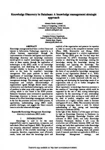
m < d, where B = AH and H is a d × m transformation matrix. According to this formalization, many common methods for linear feature extraction can be specified according to the method of deriving the transformation matrix, H. For unsupervised linear feature extraction, the most common technique is principal component analysis [5]. For this method, the columns of H consist of the eigenvectors of the d × d covariance matrix of the given patterns. It can be shown that the new features produced by principal component analysis are uncorrelated and maximize the variance retained from the original feature set [5]. The corresponding supervised technique is linear discriminant analysis. In this case, the columns of H are the eigenvectors corresponding to the nonzero eigenvalues of the matrix −1 SW SB , where SW is the within-class scatter matrix and SB is the between-class scatter matrix for the given set of patterns. Deriving H in this way maximizes the separation between class means relative to the covariance of the classes [5]. In the general case, the matrix H is chosen to maximize some criteria, typically related to class separation or classification accuracy for a specific classifier. In this view, feature selection is a special case of linear feature extraction, where the off-diagonal entries of H are zero, and the diagonal entries are either zero or one. E. Evolutionary Computation in Feature Selection and Extraction A direct approach to using GAs for feature selection was introduced by Siedlecki and Sklansky [20]. In their work, a GA is used to find an optimal binary vector, where each bit is associated with a feature (Figure 1). If the ith bit of this vector equals 1, then the ith feature is allowed to participate in classification; if the bit is a 0, then the corresponding feature does not participate. Each resulting subset of features is evaluated according to its classification accuracy on a set of testing data using a nearest-neighbor classifier [21].
0
1
0
1
is a weight associated with feature i. Each feature value is first normalized, then scaled by the associated weight prior to training, testing, and classification. This linear scaling of features prior to classification allows a classifier to discriminate more finely along feature axes with larger scale factors. A knn classifier is used to evaluate each set of feature weights. Patterns plotted in feature space are spread out along feature axes with higher weight values, and compressed along features with lower weight values. The value of k for the knn classifier is fixed and determined empirically prior to feature extraction. In a similar approach, Yang and Honavar [24] use a simple GA for feature subset selection in conjunction with DistAI, a neural network-based pattern classifier [25]. As in other GA-based feature selectors, a simple binary representation was used where each bit corresponds to a single feature. The use of the GA for feature subset selection improved the accuracy of the DistAI classifier for nearly all of the data sets explored, while simultaneously reducing the number of features considered. Their hybrid classifier, GADistAI, outperformed a number of modern classification methods on the various data sets presented. Vafaie and De Jong [26] describe a hybrid technique in which EC methods are employed for both feature selection and extraction1 in conjunction with the C4.5 decision tree classifier system [27]. Again, a binary representation is used for feature subset selection using traditional GA techniques. In this system, however, the features seen by the classifier are functions of the original features composed of simple arithmetic operations. For example, one such feature might be {(F 1 − F 2) × (F 2 − F 4)}, where F 1, F 2, and F 4 represent values from the original feature set. Here we present a new hybrid classifier loosely based on the idea of EC feature weighting. A parameterized discriminant function based on the Bayes classifier is developed, and an EC optimizer is used to tune the parameters of the new discriminant function. We show that this new hybrid system is effective at feature selection for various medical and biological data sets. II. Methods
1
d bits Feature 2 is included in the classifier. Feature 1 is not included in the classifier. Fig. 1. A d-dimensional binary vector, comprising a single member of the GA population for GA-based feature selection.
This technique was later expanded to allow linear feature extraction, by Punch et al. [22] and independently by Kelly and Davis [23]. The single bit associated with each feature is expanded to a real-valued coefficient, allowing independent linear scaling of each feature, while maintaining the ability to remove features from consideration by assigning a weight of zero. Given a set of feature vectors of the form X = {x1 , x2 , ...xd }, the GA produces a transformed set of vectors of the form X0 = {w1 x1 , w2 x2 ...wd xd } where wi
3
A. Bayesian Discriminant Functions The Bayesian classifier has a computational advantage over the previously-employed knn classifier [3] in that the training data are summarized, rather than stored. The comparison of each test sample with every known training sample to find nearest neighbors during knn classification is a computationally expensive process, even when efficient search methods are employed [28]. In contrast, finding the marginal probability associated with a particular feature value is computationally efficient for both the parametric and nonparametric forms of the Bayesian classifier. Since EC-based hybrid classifiers require many classifications to be performed during feature selection and extraction,the use of a computationally efficient classifier such as a Bayes classifier is indicated. 1 The
authors use the term “feature construction”.
4
IEEE SYMPOSIUM ON BIOINFORMATICS AND BIOENGINEERING
Unfortunately, the direct application of feature weighting as described in [1] is not effective in conjunction with the Bayes classifier, because the Bayes decision rule is invariant to linear scaling of the feature space. In other words, multiplying the feature values for a given feature by a constant has no effect on the class-conditional probabilities considered by the classifier, as illustrated in Figure 2. Direct scaling of the marginal probabilities is also ineffective for the na¨ıve Bayes classifier, since the joint class-conditional probabilities are simply the products of the marginal probability values.
the training data. Unfortunately, the search space involved 2 in finding this covariance matrix grows as 2d , even if the elements of the covariance matrix are binary-valued. For real valued matrix elements, the search space quickly becomes intractable, even for small problems. We can simplify the problem somewhat by viewing the Bayes decision rule as a discriminant function—a function g of the feature vector ~x. Consider, by way of example, a two-class decision problem. The Bayes discriminant function can be written as:
Proportion of training samples
g(~x) = P (ω1 |~x) − P (ω2 |~x)
p(x > 14, x 140, x 0, and class 2 if g(~x) < 0. The classification when g(~x) = 0 is arbitrary. The discriminant function, then, is uniquely associated with a particular classifier, mapping an input feature vector to a value associated with a particular class. According to Duda and Hart: “We can always multiply the discriminant functions by a positive constant or bias them by an additive constant without influencing the decision. More generally, if we replace every gi (x) by f (gi (x)), where f is a monotonically increasing function, the resulting classification is unchanged.” [5, pp. 17–18]. Thus, we can design a parameterized classifier based on the concept of the discriminant function. We begin with a discriminant function based on the Bayes decision rule. Using this function as a model, we can design similar functions which classify well, but are more easily parameterizable for hybridization with EC optimization methods. After designing such a discriminant function and identifying the tunable parameters, we can use an EC to optimize these parameters with regard to a particular set of training and tuning data. B. Nonlinear Weighting of the Bayes Discriminant Function Consider the Bayes discriminant function, g(~x) = =
P (ω1 |~x) − P (ω2 |~x) P (~x|ω1 ) × P (ω1 ) − P (~x|ω2 ) × P (ω2 ) 2 X P (~x|ωi ) × P (ωi )
(4)
i=1
There are, nevertheless, several aspects of the Bayesian classifier that, when optimized, can yield better classification performance. One such area is is the manner in which the marginal probabilities for each feature will be combined into the multivariate class-conditional probability densities. For the na¨ıve Bayes classifier, the class-conditional probability is the product of the marginal probabilities for each feature. A more general approach would be to encode the entire d × d covariance matrix describing the interrelationships between all the features being considered, and allow an EC-based optimizer to search for the covariance matrix which best describes the true multivariate distribution of
The denominator can be eliminated, since it does not affect the sign of g(~x), and thus does not affect the resulting classification. Since a > b ⇒ log(a) > log(b), we can apply the log function to the a posteriori probabilities without changing the resulting classification. Thus, the following discriminant function is equivalent to the na¨ıve Bayes discriminant: g(~x) =
log (P (~x|ω1 ) × P (ω1 )) − log (P (~x|ω2 ) × P (ω2 )) = (log (P (~x|ω1 )) + log (P (ω1 ))) − (log (P (~x|ω2 )) + log (P (ω2 )))
(5)
(6)
where log (P (~x|ωi )) =
log (P (x1 |ωi )) + log (P (x2 |ωi )) + ... + log (P (xd |ωi )) (7)
Finally, we can parameterize this discriminant function, while maintaining a similar level of classification accuracy, by adding coefficients to each of the marginal probabilities. P ∗ (~x|ωi ) = +
C1 log (P (x1 |ωi )) + C2 log (P (x2 |ωi )) + ... Cd log (P (xd |ωi )) + log (P (ωi )) (8)
The values for the coefficients, C1...d , are supplied by an EC optimizer. The effect of these coefficients is to apply a nonlinear weighting to each of the marginal probabilities, which are then combined to produce a confidence value, P ∗ , for each class. While P ∗ (~x|ωi ) is no longer a joint probability distribution, the discriminant function is equivalent to the na¨ıve Bayes discriminant function when C1 = C2 = ... = Cd = 1. Furthermore, the new function has several desirable features for hybridization with an EC optimizer. When a particular coefficient, Cj , is reduced to zero, the associated feature value, xj , is effectively eliminated from consideration by the classifier. This allows us to perform feature selection in conjunction with classifier tuning. Furthermore, when the value of a coefficient, Cj is increased, the marginal probability value for the associated feature, xj , has an increased influence on the value of the confidence value, P ∗ (~x|ωi ), for each class. C. Gaussian Smoothing The implementation for this discriminant function was based on the previously described nonparametric na¨ıve Bayes classifier. The marginal probability distributions for each feature were approximated using histograms with 20 bins each. A Gaussian smoothing factor was applied in order to mitigate sampling anomalies that might introduce classification bias. Given a feature value, xi , for feature i, and a class ωj , then let bωj (xi ) be the bin that xi occupies in the histogram for class ωj . When the Gaussian smoothing is applied, the effective marginal probability p(xi |ωj ) depends on the histogram value of bin bωj (xi ), as well as the histogram values of neighboring bins. Let hωj (bωj (xi )) be the histogram value for bin bωj (xi )—that is, the proportion of the training samples of class ωj that have values for feature i that belong in the bin bωj (xi )—then the effective marginal probability for feature value xi is: p(xi |ωj ) =
+σ X ¡
¢ G(k, σ) × hωj (bωj (xi ) + k)
(9)
k=−σ
where G(k, σ) is the mass density function for the Gaussian distribution at µ = 0.0, with variance σ 2 : G(k, σ) = √
1 x 2 1 e− 2 ( σ ) 2πσ
(10)
The value of σ, a run-time parameter, determines the number of bins that will contribute to each effective
5
Proportion of training samples
RAYMER ET AL.: DIMENSIONALITY REDUCTION USING GENETIC ALGORITHMS
Feature value
Fig. 3. Effects of Gaussian smoothing on the computation of effective marginal probabilities. Assuming that the current feature value falls in the center bin (black rectangle), and assuming σ = 2, then the two surrounding bins on either side (grey rectangles) also contribute to the effective marginal probability for the current feature.
marginal probability value. Figure 3 illustrates the effect of Gaussian smoothing on the effective marginal probability for a particular feature value. For the experiments detailed here, Gaussian smoothing was applied with σ = 2.0. D. GA Optimization of the Nonlinear Discriminant Coefficients Several EC-based methods were employed to optimized the coefficients of the Bayes-derived discriminant function. The experiments using a genetic algorithm as the optimizer will be described here. During the execution of the GA, each coefficient vector is passed to the classifier for evaluation, and a cost (or inverse fitness) score is computed, based primarily on the accuracy obtained by the parameterized discriminent function in classifying a set of samples of known class. Since the genetic algorithm seeks to minimize the cost score, the formulation of the cost function is a key element in determining the quality of the resulting classifier. Coefficients are associated with each term in the GA cost function that allow control of each run. The following cost function is computed by the knn classifier for each individual (consisting of a weight vector and k value): cost(w, ~ k) = + + +
Cacc × Err(w, ~ k) Cpars × nonzero(w) ~ ~ k) Cvote × incorrect votes(w, Cbal × Bal(w, ~ k)
(11)
Where Err is the error rate; nonzero(w) ~ is the number of nonzero coefficients in the discriminant function coefficient vector w; ~ and Bal is the balance, defined as the difference between the maximum and minimum classficiation accuracy among all classes. Additionally, Cacc , Cpars , and Cbal are coefficients for each of these terms, respectively. The coefficients determine the relative contribution of each part of the fitness function in guiding the GA search. The values for the cost function coefficients were determined empirically in a set of initial experiments for each data
6
IEEE SYMPOSIUM ON BIOINFORMATICS AND BIOENGINEERING
set. Typical values for these coefficients are Cacc = 20.0, Cpars = 1.0, and Cbal = 10.0.
P*(x | wj ) = C1 log (P (x1 | wj )) + C2 log (P (x2 | wj )) +
... + C4 log (P (x4 | wj )) + log (P (wj ))
E. Representation Issues and Masking W1 W2 W3 W4 M1 M2 M3 M4
The representation of the discriminant function coefficients on the chromosome is fairly direct—a 32 bit integer is used to represent each coefficient. The resulting gene on the GA chromosome yields an unsigned value over the range [0, 232 − 1]. This value is then scaled by division to yield a real value over [0.0, 100.0]. In order to infer the minimal set of features required for accurate classification, it is desirable to promote parsimony in the discriminant function – that is, as many coefficents should be reduced to zero as is possible without sacrificing classification accuracy. While the cost function encourages parsimony by penalizing a coefficient vector for each nonzero value, a simple real-valued representation for the coefficients themselves does not provide an easy means for the GA to reduce coefficients to zero. Since the GA mutation operator tends to produce a small change in a single weight value, numerous mutations of the same feature weight are often required to yield a value at or near zero. Several methods were tested to aid the search for a minimal feature set, including reducing weight values below a predefined threshold value to zero, and including a penalty term in the cost function for higher weight values. The method that proved most effective, however, was a hybrid representation that incorporates both the GA feature selection technique of Siedlecki and Sklansky [20] and the feature weighting techniques of Punch et al. [22] and Kelly and Davis [23]. In this hybrid representation, a mask field is assigned to each feature. The contents of the mask field determine whether the feature is included in the classifier (see Figure 4). In the initial implementation, a single mask bit was stored on the chromosome for each feature. If the value of this bit was 1, then the feature was weighted and included in classification. If, on the other hand, the mask bit for a feature was set to 0, then the feature weight was treated effectively as zero, eliminating the feature from consideration by the classifier. Since the masking fields comprised a very small section of the chromosome relative to the discriminant function coefficients, the number of mask bits associated with each feature was later increased to five. This increase had the effect of increasing the probability that a single bit mutation in a random location would affect the masking region of the chromosome. The interpretation of multiple mask bits is a simple generalization of the single bit case. When the majority of the mask bit values for a field are 1, then the field is weighted and included in classification. Otherwise, the field weight is reduced to 0, removing the feature from consideration by the knn. The number of mask bits is always odd so there is no possibility of a tie. Figure 4 shows a typical GA chromosome for the hybrid Bayes discriminant classifier with masking.
Fig. 4. An example of the EC chromosome for optimization of the nonlinear discriminant coefficients. A four-dimensional problem is shown. Each coefficient, Ci , in the discriminant function is determined by the chromosome weight, Wi , and the masking field, Mi .
III. Results and Discussion A. Classification of UCI Data Sets Classification of data from the UCI machine learning data set repository was performed to evaluate the effectiveness of the hybrid classifier on real-world data, and to facilitate comparison with our previously-developed hybrid EC/knn technique. The four data sets used for this evaluation are described in detail in [3], and at the UCI website [29]. Table I compares the classification and feature selection performance of the hybrid discriminant-function-based classifier with that of our previous EC/knn hybrid classifiers and the na¨ıve Bayes classifier. The most evident aspect of the results on these four data sets is the feature selection capability demonstrated by the nonlinear discriminant function. For three of the four data sets, the minimum number of features used in classification was found by the nonlinear discriminant function in conjunction with the GA. Additionally, for the hepatitis data, the test accuracy obtained by the two discriminant function classifiers surpassed the other classifiers tested. For the other three data sets the accuracies obtained by the discriminant methods were similar to those obtained by other methods tested. The notable difference between Tune and Test results for the hepatitis and ionosphere data sets suggest that the discriminant classifiers may be more prone to overfitting of the training and tuning data than the other classifiers. Examination of the run times for the UCI data sets illustrates the advantage held by the discriminant-functionbased classifiers over the EC/knn hybrid classifiers in terms of computational efficiency. Table II compares the execution times for 200 generations of GA optimization in conjunction with the nonlinear discriminant function and the knn classifier. In all cases the nonlinear discriminant classifier is significantly faster than the GA/knn—in the case of the Pima Indian diabetes data set the difference is nearly tenfold. B. Classification of Medical Data For the thyroid and appendicitis data, the discriminant function-based classifiers were trained and tested in the same manner as the previously developed EC-hybrid clas-
RAYMER ET AL.: DIMENSIONALITY REDUCTION USING GENETIC ALGORITHMS
TABLE I Results of the nonlinear-weighted Bayes discriminant function (Nonlinear) on various data sets from the UCI Machine Learning data set repository, averaged over 50 runs. Train/Tune refers to the accuracy obtained when reclassifying the data used by the EC in tuning (optimizing) feature subsets and weights. Test refers to the accuracy obtained on an independent test set for each experiment, disjoint from the training and tuning sets. The number of features is the mean number of features used in classification over all 50 runs.
Hepatitis Bayes Nonlinear GA/knn EP/knn
Train/Tune 85.3 95.4 86.0 87.2
Test 65.7 79.4 69.6 73.1
Features 19 6.5 8.1 8.9
Wine Bayes Nonlinear GA/knn EP/knn
Train/Tune 98.8 97.8 99.7 99.5
Test 94.7 91.3 94.8 93.2
Features 13 4.5 6.0 6.2
Ionosphere Bayes Nonlinear GA/knn EP/knn
Train/Tune 93.0 97.6 95.0 93.2
Test 90.1 87.5 91.9 92.3
Features 34 8.5 8.5 13.5
Pima Bayes Nonlinear GA/knn EP/knn
Train/Tune 76.1 76.2 80.0 79.1
Test 64.6 70.4 72.1 72.9
Features 8 3.9 3.1 3.9
TABLE II Execution times (wall clock time) for 200 generations of GA optimization of the knn and nonlinear discriminant function classifiers. For each data set, the number of features (d), the number of classes (C), the combined training and tuning set size (n), and the mean execution time (hours:minutes:seconds) over 50 runs are shown. Each run was executed on a single 250MHz UltraSPARC-II cpu of a six-cpu Sun Ultra-Enterprise system with 768 MB of system RAM. Runs were executed in sets of 5 with no other user processes present on the system.
Data set Pima Hepatitis Ionosphere Wine
d 8 19 34 13
C 2 2 2 3
n 400 240 400 240
knn 1:40:13 1:05:48 2:02:25 0:23:59
nonlinear 0:10:52 0:24:42 0:43:37 0:14:39
7
sifiers [3]. For each data set, five experiments were conducted for each classifier. The appendicitis data set was re-partitioned into disjoint training/tuning and testing sets for each experiment. The much larger thyroid data set was pre-partitioned into training and testing sets in the UCI database [30, ]. For this data, only the initial random GA population was changed for each experiment. The results of these experiments are summarized in Table III. TABLE III Accuracy of various classifiers on the hypothyroid and appendicitis diagnosis data sets. Results for the discriminant function classifiers are averaged over five GA experiments. Results for the GA/knn classifier represent the best of five experiments. Train/Tune refers to the accuracy obtained in reclassifying the GA tuning set; Test refers to bootstrap accuracy over 100 bootstrap sets.
Thyroid GA/knn Nonlinear Sum
Train/Tune 98.5 97.7 97.8
Test 98.4 97.2 97.4
Features 3 2.7 4.2
Appendicitis GA/knn Nonlinear Sum
Train/Tune 90.4 80.4 83.0
Test 90.6 67.0 74.2
Features 2 2.6 2.2
The discriminant function based classifier performed well on the hypothyroid diagnosis data, utilizing a smaller feature set than the GA/knn at a slight cost in bootstrap test accuracy. The poor performance of the nonlinear classifier on the appendicitis data set, along with the previous results for the hepatitis and ionosphere data sets, suggests that the discriminant function classifier may be prone to overfitting when presented with small (< 50 samples of each class) data sets for training, tuning, and testing. C. Discussion A key advantage of the discriminant function classifier over the nearest neighbor methods is the gain in computational efficiency obtained by estimating the classconditional feature value distributions based on the training data, rather than storing every training sample and performing an all-pairs search for near neighbors for each test sample. While the experiments here were all executed for a fixed number of EC generations, it would be worthwhile to run several experiments constrained instead by wall-clock time. In this way, the efficiency advantage of the discriminant function-based classifier might be translated into further gains in classification accuracy relative to the near-neighbor methods. The nonlinear discriminant function classifier, in conjunction with the GA feature extraction method, seems to exhibit the best feature selection capability of all the classifiers evaluated. In several cases, however, the additional
8
IEEE SYMPOSIUM ON BIOINFORMATICS AND BIOENGINEERING
reduction in the number of features, as compared to the GA/knn classifier, incurred a slight cost in terms of classification accuracy. The promise exhibited by the discriminant functionbased classifier suggests several avenues for further investigation. One possible improvement would be to include the prior probabilities for each class on the EC chromosome for optimization. Intuitively, this might allow the hybrid classifier more ability to maintain more control over the balance in predictive accuracy among classes, even when there is disparity in the number of training and tuning samples available for each class. Initial experimentation in this area, however, suggested that inclusion of the prior probabilities on the chromosome can exacerbate the problem of overfitting the training and tuning data, resulting in poor performance on independent test data. Since the capabilities of the Bayes classifier have been well explored in the literature, an alternate approach would be to avoid direct modification of the Bayes discriminant function. Instead, the independence assumption of the na¨ıve Bayes classifier might be abandoned, and the relationship among the various distributions of feature values encoded on the EC chromosome as a covariance matrix, or some subset thereof. Essentially, this approach would allow the EC to estimate the covariance matrix for each class based on both the training and tuning data provided. In conjunction with the previously proposed technique of including the a priori probabilities for each class on the chromosome, all the parameters of a traditional Bayes classifier might be optimized by the EC for a particular data set and error cost function.
[7]
IV. Acknowledgments We gratefully acknowledge the support of the National Science Foundation (grant DBI-9600831 to L.K.) for this research. M.R. would also like to thank Drs. Erik Goodman and Rich Enbody for their assistance and critical feedback.
[8]
[9] [10]
[11] [12] [13] [14]
[15]
[16] [17]
[18] [19] [20] [21] [22]
[23]
References [1]
[2]
[3]
[4] [5] [6]
M. L. Raymer, P. C. Sanschagrin, W. F. Punch, S. Venkataraman, E. D. Goodman, and L. A. Kuhn, “Predicting conserved water-mediated and polar ligand interactions in proteins using a k-nearest-neighbors genetic algorithm,” J. Mol. Biol., vol. 265, pp. 445–464, 1997. M. L. Raymer, W. F. Punch, E. D. Goodman, P. C. Sanschagrin, and L. A. Kuhn, “Simultaneous feature scaling and selection using a genetic algorithm,” in Proc. Seventh Int. Conf. Genetic Algorithms (ICGA), Th. B¨ ack, Ed., San Francisco, 1997, pp. 561–567, Morgan Kaufmann Publishers. M. L. Raymer, W. F. Punch, E. D. Goodman, L. A. Kuhn, and A. K. Jain, “Dimensionality reduction using genetic algorithms,” IEEE Transactions on Evolutionary Computing, vol. 4, no. 2, pp. 164–171, 2000. T. Bayes, “An essay towards solving a problem in the doctrine of chances,” Phil. Trans. Roy. Soc., vol. 53, 1763. R. O. Duda and P. E. Hart, Pattern Classification and Scene Analysis, John Wiley & Sons, 1973. P. Domingos and M. Pazzani, “Beyond independence: Conditions for the optimality of the simple bayesian classifier,” in Proceedings of the Thirteenth International Conference on Machine Learning, Lorenza Saitta, Ed., San Francisco, CA, 1996, pp. 105–112, Morgan Kaufmann.
[24]
[25]
[26]
[27]
[28] [29]
E. T. Jaynes, “Prior probabilities,” in IEEE Transactions on Systems Science and Cybernetics, 1968, vol. SSC-4, pp. 227–241. A. K. Jain and B. Chandrasekaran, “Dimensionality and sample size considerations in pattern recognition in practice,” in Handbook of Statistics, P. R. Krishnaiah and L. N. Kanal, Eds. 1982, vol. 2, pp. 835–855, North-Holland. G. V. Trunk, “A problem of dimensionality: A simple example,” IEEE Transactions on Pattern Analysis and Machine Intelligence, vol. 1, pp. 306–307, 1979. T. M. Cover and J. M. Van Campenhout, “On the possible orderings in the measurement selection problem,” IEEE Transactions on Systems, Man, and Cybernetics, vol. 7, pp. 657–661, 1977. P. M. Narendra and K. Fukunaga, “A branch and bound algorithm for feature subset selection,” IEEE Transactions on Computers, vol. C-26, pp. 917–922, 1977. A. Whitney, “A direct method of nonparametric measurement selection,” IEEE Transactions on Computers, vol. 20, pp. 1100– 1103, 1971. P. Pudil, J. Novovicova, and J. Kittler, “Floating search methods in feature selection,” Pattern Recognition Letters, vol. 15, pp. 1,119–1,125, Nov. 1994. A. K. Jain and D. Zongker, “Feature selection: Evaluation, application, and small sample performance,” IEEE Transactions on Pattern Analysis and Machine Intelligence, vol. 19, no. 2, pp. 153–158, February 1997. J. Mao, K. Mohiuddin, and A. K. Jain, “Parsimonious network design and feature selection through node pruning,” in Proc. of the Intl. Conf. on Pattern Recognition, Jerusalem, October 1994, pp. 622–624. K. Nozaki, H. Ishibuchi, and H. Tanaka, “Adaptive fuzzy rulebased classification systems,” IEEE Transactions on Fuzzy Systems, vol. 4, no. 3, pp. 238–250, August 1996. H. Ishibuchi, K. Nozaki, N. Yamamoto, and H. Tanaka, “Selecting fuzzy if-then rules for classification problems using genetic algorithms,” IEEE Transactions on Fuzzy Systems, vol. 3, no. 3, pp. 260–270, August 1995. J. R. Quinlan, “Induction of decision trees,” Machine Learning, vol. 1, pp. 81–106, 1986. J. R. Quinlan, “Simplifying decision trees,” International Journal of Man-Machine Studies, pp. 221–234, 1987. W. Siedlecki and J. Sklansky, “A note on genetic algorithms for large-scale feature selection,” Pattern Recognition Letters, vol. 10, pp. 335–347, 1989. T. M. Cover and P. E. Hart, “Nearest neighbor pattern classification,” IEEE Transactions on Information Theory, vol. IT-13, pp. 21–27, 1967. W. F. Punch, E. D. Goodman, M. Pei, L. Chia-Shun, P. Hovland, and R. Enbody, “Further research on feature selection and classification using genetic algorithms,” in Proc. International Conference on Genetic Algorithms 93, 1993, pp. 557–564. J. D. Kelly and L. Davis, “Hybridizing the genetic algorithm and the k nearest neighbors classification algorithm,” in Proceedings of the Fourth International Conference on Genetic Algorithms and their Applications, 1991, pp. 377–383. J. Yang and V. Honavar, “Feature subset selection using a genetic algorithm,” in Feature Extraction, Construction and Selection: A Data Mining Perspective, H. Liu and H. Motoda, Eds., chapter 8, pp. 117–136. Kluwer Academic Publishers, Norwell, MA, 1998. J. Yang, R. Parekh, and V. Honavar, “DistAI: an inter-pattern distance-based constructive learning algorithm.,” in Proceedings of the International Joint Conference on Neural Networks, Anchorage, Alaska, 1998. H. Vafaie and K. De Jong, “Evolutionary feature space transformation,” in Feature Extraction, Construction and Selection: A Data Mining Perspective, H. Liu and H. Motoda, Eds., chapter 19, pp. 307–323. Kluwer Academic Publishers, Norwell, MA, 1998. J. R. Quinlan, “The effect of noise on concept learning,” in Machine Learning: an Artificial Intelligence Approach, R. Michalski, J. Carbonnell, and T. Mitchell, Eds., pp. 149–166. Morgan Kaufmann, 1986. K. Fukunaga and P. M. Narendra, “A branch and bound algorithm for computing k-nearest neighbors,” IEEE Transactions on Computers, pp. 750–753, 1975. C. L. Blake and C. J. Merz, “UCI repository of machine learning databases,” University of California, Irvine,
RAYMER ET AL.: DIMENSIONALITY REDUCTION USING GENETIC ALGORITHMS
Dept. of Information and Computer Sciences, 1998, http://www.ics.uci.edu/∼mlearn/MLRepository.html. [30] J. R. Quinlan, P. J. Compton, K. A. Horn, and L. Lazurus, “Inductive knowledge acquisition: A case study,” in Proceedings of the Second Australian Conference on Applications of Expert Systems, Sydney, Australia, 1986.
9